                  Word                  Tokens
1                 data                    data
2        statistics101        statistics | 101
3 internationalization international | ization
4              running              run | ning
5 better better19 Working with Large Language Models (LLMs) and Agentic Systems
Keywords
LLMs, Prompt Engineering, Tokenization, Agentic Systems, Context Engineering, LLM Agents, Ollama, OpenAI SDK, Claude Code, Positron Assistant
19.1 Introduction
19.1.1 Learning Outcomes
By the end of this section, you should be able to:
19.1.2 Learning Outcomes
By the end of this chapter, you should be able to:
Prompts and Language Models
- Describe how large language models generate responses, including the role of tokenization, token limits, and how model size affects output quality and consistency
- Develop effective prompts for interactive chat, distinguishing between one-off queries and prompts designed for reuse in code
- Convert a well-designed chat prompt into a reusable, parameterized function suitable for embedding in a larger analytical system
- Design prompts that provide sufficient context for agentic systems, including role, task, constraints, and examples
Workflows and Agents with Local Models
- Explain the difference between a prompt, a workflow, and an agentic system, and identify which is appropriate for a given task
- Call a local language model from R using Ollama and treat it as a function inside a larger program
- Build a generate -> evaluate -> revise loop and explain why evaluation is a prerequisite for reliable agentic behavior
- Define deterministic and prompt-based tools and register them in a tool registry that the model can select from at runtime
- Construct a balanced agent with a layered architecture: core model interface, shared helper functions, generate/evaluate tool pairs, and an orchestration loop
- Apply context engineering principles to multi-call systems; deciding what information each model call needs and what to leave out
- Extend a balanced agent with persistent memory and a pipeline wrapper to handle multi-step tasks that depend on intermediate results
- Debug failures in prompts, code execution, and tool selection using structured debug logs
Working with Cloud APIs and Agent Frameworks
- Swap a local Ollama model for a cloud-hosted model (e.g., Groq) by changing a single configuration file, demonstrating that the balanced agent architecture is model-agnostic
- Identify the tradeoffs between building your own agent with a cloud API, using an agent SDK or framework, and directing an opinionated agent system
- Build and run a Python agent using the OpenAI Agents SDK, including defining tools with the
@function_tooldecorator, writing effective tool docstrings, and running the agent loop withRunner.run_sync() - Interpret OpenAI platform traces to understand what the model received, which tools it called, and what each step cost in tokens and time
- Fetch and cache real-world government data from the NYC Open Data Socrata API and apply it across multiple agent approaches
Opinionated Agentic Systems
- Configure and use Claude Code in the terminal, including setting up CLAUDE.md project context, defining skills and subagents, and managing the Git workflow from within a session
- Explain the permission model for Claude Code, the distinction between Allow (code execution) and Keep (file modification), and apply it deliberately
- Compose a team of specialized subagents (e.g., viz-specialist, data-scientist) and explain the token-economy benefits of delegating to isolated context windows
- Configure Positron Assistant with a Console API key, connect GitHub Copilot for inline completions, and use Ask, Edit, and Agent modes for different kinds of analytical tasks
- Explain what Positron Assistant knows about your session that a terminal-based agent does not, and use that session awareness to ask more precise analytical questions
- Apply responsible use principles specific to agentic systems: minimum necessary scope, human checkpoints before irreversible actions, critical evaluation of agent output, and transparency about AI assistance in submitted work
19.1.3 References
- OpenAI’s Prompt Engineering (OpenAI 2025)
- Prompt Engineering Guidebook (DAIR-AI 2025)
- Prompt Engineering Overview (Anthropic Engineering, n.d.-a)
- Effective context engineering for AI agents (Anthropic Engineering 2025)
- OLlama (“Ollama’s Documentation” 2026)
- Building Effective AI Agents (Anthropic 2024)
- A practical guide to building agents [aopenaiPracticalGuideBuilding2026]
- Socrata Open Data Network and API (Socrata Developers, n.d.)
- Groq API Reference (groq, n.d.)
- OpenAI Agents SDK Documentation (OpenAI Developers, n.d.)
- Claude Code Documentation (Anthropic, n.d.-b)
- VoltAgent Awesome Claude Code Subagents (VoltAgent/Awesome-Claude-Code-Subagents 2026)
- Positron (Posit 2025)
- Positron Assistant (Positron, n.d.)
R and Python Packages
- RSocrata - an R package for Socrata Open Data Portals (City of Chicago, n.d.)
- {tidycensus} R Package (Walker and Herman 2023)
- {keyring} R Package (Csardi 2022)
- pyprojroot: Project-oriented workflow in Python (Chen 2026)
- {pdfplumber} python package for working with PDFs (Jeremey Singer-Vine, n.d.)
- Definitive Guide to pdfplumber Text and Table Extraction Capabilities (Bispo 2024)
Other References for additional exploration.
- Both OpenAI and Anthropic have many online resources for supporting the use of their agentic systems as do other LLM providers.
- Best Practices for CLaude (Anthropic, n.d.-a)
- Prompting Best Practices (Anthropic Engineering, n.d.-b)
- Introduction to CLaude Skills (Alex Notov 2025)
- How to Build a Production-Ready Claude Code Skill (Takeda 2026)
- Claude Code: Create custom subagents (“Claude Code Create Custom Subagents,” n.d.)
- Claude Code: Define your agent (“Claude Code Define Your Agent,” n.d.)
- Google Agent Development Kit (ADK) (Google, n.d.)
- {uv} Python Package Manager (Astral 2025)
- OWASP Least Privilege Principle (OWASP Foundation, n.d.)
Academic literature on LLM agents and prompt engineering
- A Systematic Survey of Prompt Engineering in Large Language Models: Techniques and Applications (Sahoo et al. 2024) covers techniques from zero-shot and few-shot prompting through chain-of-thought.
- A Survey of Context Engineering for Large Language Models (Mei et al. 2025) introduces context engineering as a formal discipline distinct from prompt engineering, covering retrieval, memory, tool integration, and multi-agent systems across 1,400 papers.
- Agentic Large Language Models, a survey (Plaat et al. 2025) covers LLMs that reason, act, and interact, organized around exactly those three capabilities, with discussion of tool use, multi-agent systems, and responsible use risks.
- Large Language Model Agent: A Survey on Methodology, Applications and Challenges (Luo et al. 2025) covers agent architectures, collaboration mechanisms, and evaluation methodologies with a unified taxonomy.
- Awesome Agent Papers (Luo 2026) The companion repository to the survey above, maintained as a curated and continuously updated reading list organized by the same taxonomy. A good starting point for going deeper on any specific topic from this chapter.
NoteA Note on the Development of This Chapter
This chapter was developed with the assistance of both ChatGPT and Claude.
- These tools were used throughout to explore ideas, generate initial code, and draft prose.
- Through extended iterative conversations the material was revised, restructured, removed, and adjusted as I tuned it to align with my pedagogical goals for this course and serve as a reference for others.
- All material was verified against primary references. The framing, sequencing, and editorial judgments are my own.
The contents of this chapter, their clarity, accuracy, and relevance, are my responsibility. Any errors are mine alone.
19.2 A Guide to Prompt Engineering
Note
This section was written based on a conversation with an AI Assistant that started with a 156 word prompt and about 25 follow-up prompts to adjust, expand and refine content. Additional human editing improved clarity and consistency as well as formatting and adjustments to code and code chunk options. References were checked and adjusted for accuracy and citations were added. Links to inline references were added. Any errors are my responsibility.
19.2.1 Prompt Engineering
“Prompt engineering is the process of writing effective instructions for a model, such that it consistently generates content that meets your requirements.” OpenAI (2025)
A “prompt” can be a question, a request for code, a set of instructions, or even an ongoing conversation with a Large Language Model (LLM).
- Creating or “engineering” a prompt (or series of prompts) to produce the most accurate, useful, and relevant output possible to meet your goals is still a mix of art and science.
Prompt engineering builds on an understanding of how LLMs work (not how they are trained) to create prompts that are effective for your purposes. Characteristics of LLMs can shape effective prompts.
- Non-determinism: LLM responses vary because they are generated from probabilities in a high-dimensional space. Small wording changes can produce very different outputs.
- Asking what is the “most positive” versus the “least negative” sentiment of text.
- Context Sensitivity: LLMs don’t “understand” in the human sense; they generate responses based on patterns in data. How you ask a question strongly influences the quality of the answer.
- Specifying “Give me R code” versus “Explain in plain English” leads to very different outputs.
You can apply guidelines and best practices to improve your chances of getting useful results consistently while building your understanding and skills.
- Efficiency: A well-crafted prompt reduces the need for repeated clarifications.
- Accuracy: Clear context, guidance, and constraints can help minimize errors or hallucinations.
- Improved Collaboration: prompt engineering can be seen as refining or debugging your question prior to collaborating with others or the LLM.
- Multi-language skill: The same techniques apply whether you’re generating R code, Python code, documentation, or explanations.
In short: Prompt engineering is about learning how to “talk to the model” effectively so it can become a productive tool for your goals rather than a source of confusion.
19.2.2 How LLMs Respond to Prompts
LLMs (like ChatGPT, Claude, or Gemini) do not “understand” like humans. Instead, they:
- Predict the next token (word or subword) given your input and context.
- Use patterns from training data to approximate reasoning.
- Are sensitive to framing: wording, order, specificity, and constraints change the output.
- Can hallucinate: generate confident-sounding but false statements.
19.2.2.1 Tokenization
LLMs do not read raw text directly. Instead, they break text into tokens (smaller units such as words, subwords, or characters).
- Tokens are not always whole words.
- Example:
"data science"→["data", " science"](2 tokens)
- Example:
"statistics101"→["statistics", "101"](2 tokens)
- Example:
"internationalization"→["international", "ization"](2 tokens)
- Example:
- This is similar to but not the same as Lemmatization which reduces words to their base form (common in NLP preprocessing, not in LLM tokenization).
"running"→"run"
"better"→"good"
Here is a toy example of token splitting.
19.2.2.2 The Context Window and Token Limits and Conversation Context
The context window is the full set of tokens the model sees at any single moment — think of it as the model’s working memory for a task.
- It holds everything at once: your system instructions, the conversation history, your current message, and any retrieved documents or data.
- The model can only reason about what is currently in this window.
- Nothing outside it exists from the model’s perspective.
- Managing what goes into this window (what to include, what to summarize, what to leave out) becomes one of the most important skills as you move from interactive chat toward writing code that calls models programmatically.
Each model has a maximum token limit (prompt + response combined).
- Context windows have grown dramatically and continue to expand rapidly so always check the current documentation for the model you are using.
- Representative sizes as of early 2026:
- Small/local models (e.g., ollama 7B–13B): 8k–32k tokens
- Mid-range models (e.g., GPT-4o, Llama 3.1): 128k tokens
- Large frontier models (e.g., Claude Sonnet 4.6, Gemini 3 Pro, GPT-5.4): 200k–1M+ tokens
How “memory” actually works in interactive chat:
- The model itself is stateless, i.e.,it has no built-in memory between calls.
- Each API call is processed independently, with no knowledge of prior exchanges unless that history is explicitly included.
- The appearance of a continuous conversation is an illusion created by the application layer (Claude.ai, ChatGPT, etc.), which automatically prepends all prior messages to each new prompt before sending it to the model.
- As a conversation grows, so does the context it consumes.
- Long conversations with code in prompts and responses can fill the context window quickly and slow performance.
- If the limit is approached, older context may be truncated, leading to loss of information or inconsistent responses and eventually you will need to start a new conversation.
Bigger is not always better — context rot:
- Research consistently shows that model performance degrades as context length increases, even when the tokens technically fit in the window. This is sometimes called context rot.
- Models tend to attend more reliably to information near the beginning or end of the context, and may lose track of details buried in the middle.
- More tokens can mean more distraction, not more capability.
- A practical rule of thumb: effective reliable performance is typically lower than the advertised maximum.
Persistent memory is a different mechanism entirely:
- Some platforms (e.g., Claude Projects, ChatGPT’s memory feature, Gemini’s notebook integrations) now offer persistent memory which is the ability to retain information across separate conversations.
- This is not a property of the model itself. It is an application-layer feature: the platform stores summaries or preferences externally and injects them back into the context window at the start of each new session.
- The underlying model is still stateless; what changes is what the platform loads into context before you say a word.
- Systems such as Retrieval-Augmented Generation (RAG) and augmented LLMs Section 19.4.1, exhibit this pattern of storing information externally and retrieving it into context on demand.
- These are examples of persistent memory scaliung from a chat interface feature into a key element of agentic systems.
TipBest practices to manage your context window
- Keep prompts focused. Paste only the relevant portion of a dataset or file, not the whole thing. Summarize or sample when the input is large.
- Start a new conversation for a new topic. This prevents unrelated context from accumulating and keeps the window clean.
- For local models with smaller windows (as you will use with ollama), this constraint is tighter so short, targeted prompts matter more.
- Place the most important information at the beginning of your prompt, not buried in the middle, where attention is weakest.
19.2.2.3 Tokens are Converted to Numbers
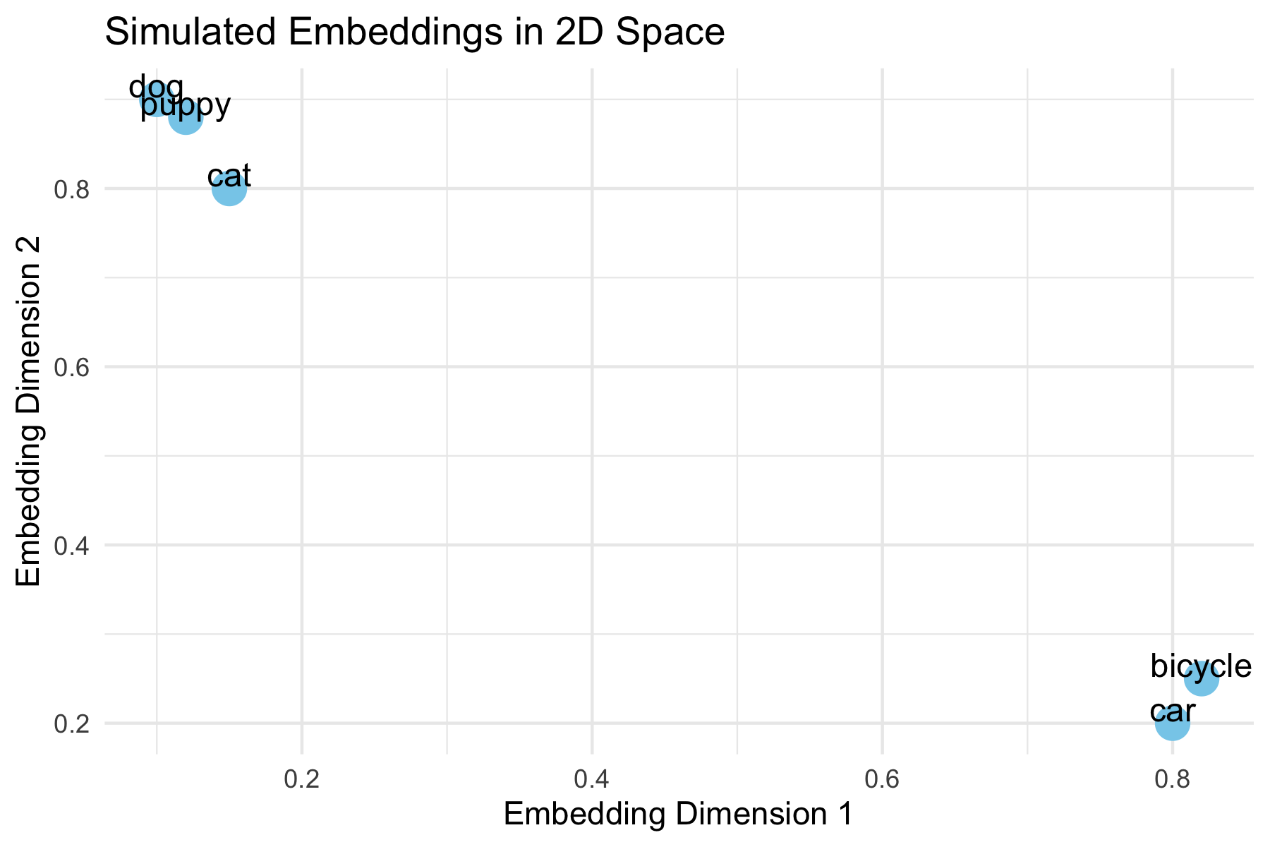
- LLMs do not operate on tokens as text. Each token is mapped to a numerical vector (an embedding).
- Embeddings are high-dimensional vector representations of tokens or text that capture semantic meaning.
- LLM embeddings are vectors with hundreds or thousands of dimensions, not just 2 or 3, and each dimension encodes some aspect of meaning, context, or syntactic/semantic feature.
- Different models can use different embedding schemes.
- The model performs mathematical operations on these vectors to predict the next token based on mathematical similarity or “closeness.”
Example:
- "dog" → [0.12, -0.03, 0.88, ...]
- "puppy" → [0.14, -0.01, 0.91, ...]
- "car" → [0.80, 0.20, -0.05, ...]
19.2.3 Measuring Closeness
Similarity between the embedding vectors is measured using metrics like cosine similarity.
\[ \text{cosine similarity} = \frac{\vec{A} \cdot \vec{B}}{\|\vec{A}\| \|\vec{B}\|} \]
- Cosine similarity = 1 -> vectors point in the same direction (highly similar meaning).
- Cosine similarity = 0 ->vectors are orthogonal (unrelated meaning).
Embeddings allow LLMs to “understand” similar words or phrases as they have embeddings “close” together in vector space.
- These metrics are used for:
- Semantic search (finding relevant text)
- Retrieval-Augmented Generation (RAG)
- Clustering or similarity calculations
- Semantic search (finding relevant text)
19.2.4 Visualizing Embeddings in R
This example shows how words with similar meaning might cluster together in the embedding space.
- “dog”, “puppy”, and “cat” cluster closely, reflecting semantic similarity.
- “car” and “bicycle” are farther away, showing unrelated meaning.
- In real embeddings, vectors are high-dimensional, but this 2D example illustrates the concept.
- Cosine similarity measures closeness mathematically in high dimensions, even though they can’t be plotted.
Warning
Important nuance
- These similarity measures are inherently fuzzy.
- Minor variations in your prompt—such as negating a sentence, reordering words, or changing context—can result in large differences in the output, even if the overall meaning seems similar to a human reader.
Example:
- Prompt 1: "List three common R functions for plotting a histogram."
- Prompt 2: "List three uncommon R functions for plotting a histogram."
- Prompt 3: "List three popular R functions for plotting a histogram."
Even though only one word changes, the model may:
- Suggest completely different functions.
- Reorder examples differently.
- Include/exclude certain packages.
This happens because embeddings map text to points in a continuous space, and the model predicts outputs based on small differences in those positions.
Takeaway: Always experiment with multiple phrasings and verify results. Treat embeddings and similarity measures as guides, not exact truth.
19.2.5 Guidelines for Effective Prompts
Good prompts share a few common traits: they are clear, contextual, and iterative. Here are strategies to improve your interactions with AI tools:
- Be Specific
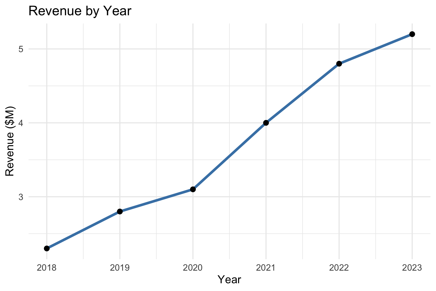
Clearly describe what you want the AI to do. Include the programming language, the type of output, and the level of detail you expect.
Example:- Weak: “Plot the data.”
- Strong: “Write R code using ggplot2 to create a line plot of
revenuebyyearwith labeled axes and a descriptive title.”
- Give Context
Provide background information such as the data structure, libraries, or your end goal. This reduces ambiguity and helps the AI tailor its response.
Example:- “I have a pandas data frame with columns
cityandpopulation. Please write Python code using seaborn to create a bar chart of population by city.”
- “I have a pandas data frame with columns
- State Constraints
Specify limitations or requirements for the response, such as the format, length, or assumptions.
Example:- “Give me only the R code, no explanations.”
- “Limit the answer to a single ggplot2 figure.”
- “Assume the data frame has no missing values.”
- Iterate
Think of prompting as a conversation, not a one-shot request. Start simple, review the output, and refine with follow-up prompts.
Example:- First prompt: “Write Python code to read a CSV file and display the first five rows.”
- Follow-up: “Now extend this code to calculate the mean of all numeric columns.”
- Next follow-up: “Format the summary as a neat table.”
- Later, we will see how iteration moves from conversation to code, where you can reuse a prompt programmatically rather than by typing.
- Verify
Never assume the AI is correct. Check the output against your own knowledge, official documentation, or by running the code. Be alert for hallucinations (nonexistent functions, incorrect syntax, or misleading explanations).
Example:- If the AI suggests
robust_cor()in R, search the documentation. If it doesn’t exist, redirect:
“That function doesn’t exist. Could you instead use Spearman’s correlation or show me how to fit a robust regression withMASS::rlm()?”
- If the AI suggests
- Adjust for Creativity or Accuracy
You can control how wide-ranging or precise the response should be by adjusting your wording.
Example:- Creative: “Show three different ways in R to visualize a distribution.”
- Accurate: “Show the single most standard ggplot2 approach for plotting a histogram of a numeric variable.”
- Assign a Role
Guide the style of the response by telling the AI who it should act as.
Example:- “You are a data science tutor. Explain correlation to a beginner and include an R code example.”
- “You are a coding assistant. Provide concise Python code with no explanations.”
19.2.5.1 Example: Making a Good First Prompt
Weak prompt:
> Plot the data.
Improved prompt:
> I have a data frame in R with columns year and revenue. Please write R code using ggplot2 to create a line plot of revenue by year, with labeled axes and a title.
19.2.5.2 Example: Building a Conversation
First Prompt:
> Write Python code to read a CSV and summarize the first five rows.
LLM Output:
Code using pandas.read_csv() and df.head().
Follow-Up Prompt:
> Please extend your code to also compute the mean of all numeric columns and print the result.
LLM Output:
Adds df.mean(numeric_only=True).
Next Follow-Up:
> Could you format the summary as a table with column means below the head output?
The model refines until the solution fits your needs.
19.2.5.3 Example: Checking for Hallucinations
Prompt:
> Write R code to compute a robust correlation coefficient.
LLM Output:
Provides code with a function robust_cor() (a hallucination as the function does not exist).
Student Check: - Get’s an error message and looks up if robust_cor() exists in R.
- If not, ask:
> That function doesn’t seem to exist. Could you instead show how to use MASS::rlm() or another real package to compute robust correlation?
The key is to verify and redirect.
19.2.5.4 Example: Large vs. Small Model Responses
The same prompt can yield different results depending on the size of the model.
Larger models (billions of parameters) generally produce more detailed and accurate answers, while smaller ones may be faster but less reliable.
Prompt:
> In R, how do I compute the correlation between two variables when the data has outliers?
| Model | Response |
|---|---|
| Large model (e.g., GPT-4, Claude Opus, Llama-70B) | “One option is to use a robust correlation method. For example, you can use Spearman’s rank correlation in R: cor(x, y, method = "spearman"). Another approach is to fit a robust regression using MASS::rlm() if you want to downweight outliers. Both approaches reduce the influence of extreme values compared to Pearson correlation.” |
| Smaller model (e.g., GPT-3.5, Llama-7B) | “You can use cor(x, y) in R. This computes correlation between two vectors.” (Note: does not mention outliers or alternatives like Spearman or robust regression.) |
Takeaway:
- The large model recognizes the nuance (outliers) and suggests multiple valid approaches.
- The smaller model gives a quick but incomplete response.
- Lesson: Always check whether the model has considered your context.
19.2.5.5 Example: Specifying Roles
When prompting, you can assign a role to the AI which will adjust its response.
Prompt 1 (role: assistant):
> You are a coding assistant. Write R code to plot the distribution of a numeric variable.
Likely Response:
Straightforward R code using hist() or ggplot2::geom_histogram().
Prompt 2 (role: instructor):
> You are a statistics instructor. Explain to a beginner how to plot the distribution of a numeric variable in R, and include an example using ggplot2.
Likely Response:
A step-by-step explanation with annotated code — more teaching-oriented.
19.2.5.6 Example: Adjusting Creativity vs. Accuracy
LLMs can be “dialed” for creativity (diverse answers, new ideas) or accuracy (precise, more deterministic answers).
- This is often controlled by a setting called temperature (higher = more creative, lower = more predictable).
- Even without changing system settings, you can influence style through your prompt wording.
Prompt (creative mode):
> Be imaginative. Show me three different R approaches to visualize the distribution of a variable.
Possible Output:
- Histogram (geom_histogram())
- Density plot (geom_density())
- Boxplot (geom_boxplot())
Prompt (accuracy mode):
> Provide the single most standard way in R using ggplot2 to visualize a variable’s distribution.
Possible Output:
One clean example using geom_histogram(), without alternatives.
Below we show a “standard” accurate plot of a distribution: If the AI had been asked in creative mode, it might instead show a density plot, violin plot, or boxplot.
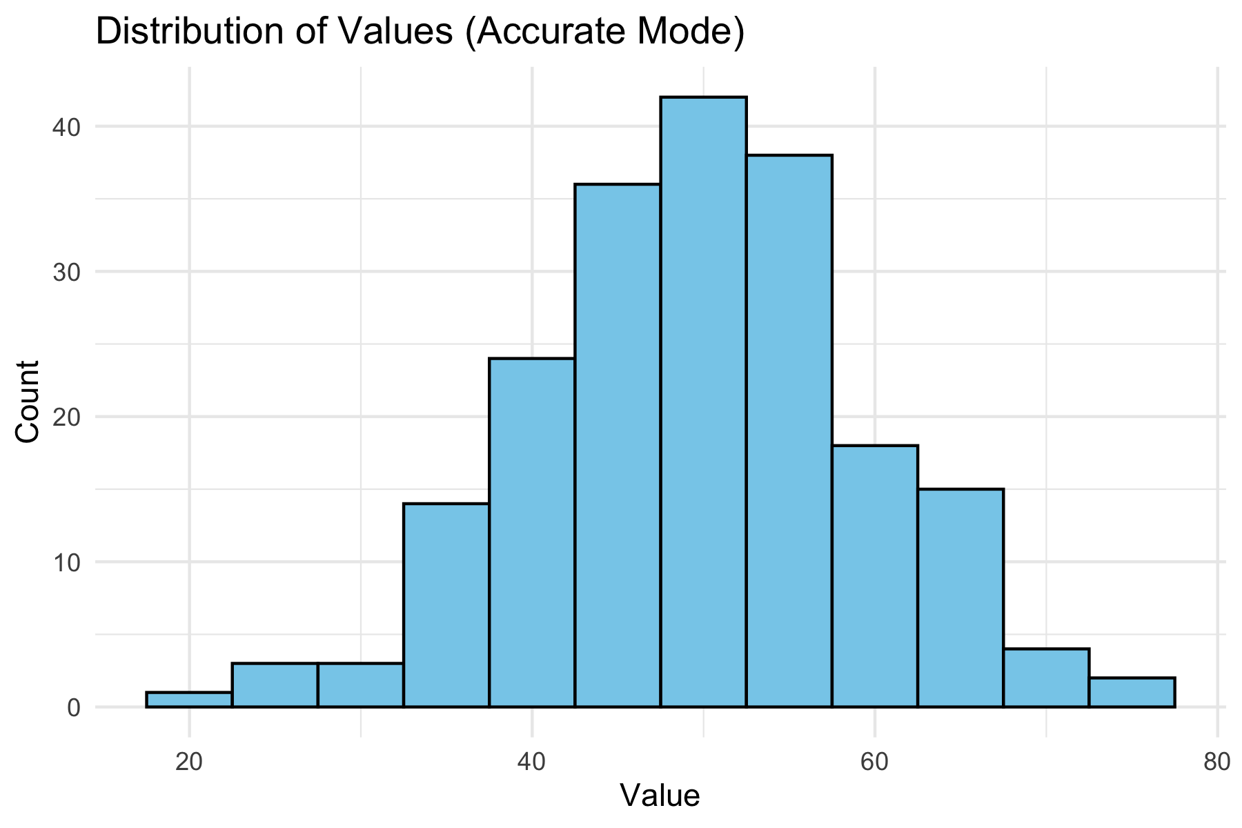
You can shape the AI’s “persona”(assistant, instructor, critic, tutor) and also control breadth vs. precision of answers depending on their goals.
19.2.6 Summary
Here is a quick reference sheet you can use when working with AI tools:
| Strategy | What It Means | Example Prompt |
|---|---|---|
| Specify Role | Tell the AI who it should act as (assistant, instructor, critic, tutor). | “You are a statistics instructor. Explain correlation to a beginner with examples in R.” |
| Give Context | Provide background: dataset, libraries, goals. | “I have a data frame in R with columns year and revenue. Use ggplot2 to plot revenue by year.” |
| State Constraints | Limit length, format, or assumptions. | “Give me Python code only, no explanations, using pandas and seaborn.” |
| Iterate | Use follow-up prompts to refine or extend. | “Now add labels to the axes.” |
| Verify | Check outputs against your knowledge or documentation. | “That function doesn’t exist in R. Show me an alternative from MASS or robustbase.” |
| Creativity vs. Accuracy | Ask for one best method (accuracy) or multiple diverse methods (creativity). | “Show three different ways in R to visualize a distribution.” |
| Check for Hallucination | Be skeptical if the AI invents code/functions. Redirect if necessary. | “I can’t find that function. Can you cite the package or suggest a real function?” |
Prompt engineering is not about tricking the AI, but about effective communication.
Think of the AI as a partner: - You provide structure, clarity, and verification. - It provides suggestions, alternatives, and explanations.
With practice, you’ll learn when to ask for creativity, when to demand precision, and how to iterate toward a reliable solution.
In the next section, we begin moving from interactive conversations to code driven interactions, turning prompts from typed messages into functions that can be called, tested, and reused.
19.3 From Interactive Prompts to Code
This short module is about transitioning from chat-based interactions to working with LLMs in a structured, code-driven manner as is required for agentic systems.
It focuses on strengthening thinking about prompts in three areas that will be useful for using agents:
- Structured prompt design
- Iteration as a loop
- Constraint prioritization
19.3.1 A Simple Prompt Template
The following template provides a consistent way to construct high-quality prompts.
A good prompt answers five questions:
- ROLE: Who should the AI act as?
- TASK: What exactly should it do?
- CONTEXT: What information does it need?
- CONSTRAINTS: What rules must it follow?
- OUTPUT FORMAT: What should the result look like?
Example:
- Role: You are a data science tutor.
- Task: Write R code to visualize revenue over time.
- Context: I have a data frame with columns
yearandrevenue. - Constraints:
- Use ggplot2
- Assume no missing values
- Include axis labels and a title
- Output: Code only with no explanation
The ROLE component deserves particular attention because it shapes the entire character of the response — and because in more complex systems, the same model may be called multiple times playing different roles within a single workflow.
- Role prompting reliably affects output style and format across models. Its effect on accuracy is less consistent and depends on the model and task.
- The most reliable use of roles in data science workflows is not to improve correctness, but to separate concerns by using different roles to shape what the model attends to and how it presents results.
NoteCommon roles and what they signal to the model
Table 19.1 lists some common roles you can use to shape the LLM response style and structure in lieu of lengthy prose descriptions.
| Role | Primary Effect | Example use |
|---|---|---|
| Coding assistant | Terse, code-first, no explanation | Generating a function |
| Data science tutor | Explanatory, step-by-step, teaching tone | Learning a new method |
| Code reviewer | Critical framing, error-focused | Evaluating output quality |
| Planner | Breaks a task into ordered subtasks | Decomposing a complex goal |
| Evaluator / Judge | Assesses output against criteria | Checking constraint satisfaction |
| Summarizer | Condenses prior context | Compressing conversation history |
These role serve distinct purposes:
- The first three roles primarily change style and are broadly consistent across models.
- The last three, Planner, Evaluator, and Summarizer, are structural roles used to divide labor across separate model calls.
- These are where role assignment matters most in agentic systems:
- Asking the same model call to both generate and evaluate its own output in one prompt is less reliable than separating those roles into two calls.
A tightly structured prompt has the following benefits:
- Reduced ambiguity
- Improved consistency which supports reproducibility
- Easier to debug
- Provides a foundation for agentic systems
This structure mirrors how agentic systems internally organize tasks, making it easier to transition from prompting to automated workflows.
19.3.2 Iteration as a Loop
In chat-based interactions, iterating prompts can be thought of as a conversation.
However, when working with code-driven interactions, it is more useful to think of iteration as a structured loop.
The Iteration as a Structured Loop Pattern follows a common cycle:
- Ask
- Evaluate
- Refine
- Repeat
Example
- Ask: Write R code to plot revenue by year.
- Evaluate: Check for missing labels or no title
- Refine: Add axis labels and a descriptive title.
- Repeat: Continue refining until the output meets requirements
This loop is the foundation of more advanced systems:
- Interactive Prompting leads to a human-driven manual loop
- Workflows can automate a fixed version of this loop
- Agents can run it dynamically, deciding when to continue, stop, or change direction.
19.3.3 Constraint Hierarchy
Not all constraints are equally important. Focus on the critical few instead of the “messy many.”
Suggested: Prioritize Constraints in the following order and check constraints in this order as errors are often caused by missing or unclear high-priority constraints.
- Output Goal
- code vs explanation
- table vs paragraph
- Tools / Libraries
- ggplot2, pandas, etc.
- Assumptions
- missing values
- data types
- Scope
- one solution vs multiple options
- Style
- concise vs detailed
Example of weak versus strong:
- Weak constraint: Make it clear and nice.
- Strong constraint: Output only R code using ggplot2 with labeled axes and a title.
Example: Poor vs Structured Iteration
- Poor Iteration: User repeatedly adds vague follow-ups such as “Make it better”, “Fix it” or “Change it a bit”
- Results can be inconsistent outputs, drifting logic, confusion in tracking the logical flow.
- Improved Approach:
- Reset with structure:
- You are a coding assistant.
- Task: Create a ggplot line chart.
- Context: Data frame with year and revenue.
- Constraints: Use ggplot2, include labels and title
- Output: Code only
- Then iterate systematically using the loop.
- Reset with structure:
The key difference is not more prompts, but better structure in each prompt.
TipInput Constraints Inform Error Checking and Evalation Tests on Output
Constraints are not just input instructions, they also inform tests for whether the output is correct”.
Well-designed constraints make it easier to identify problems such as:
- missing required elements
- incorrect format
- use of the wrong tools or libraries
- logically inconsistent results
Example prompt with weak constraints: Plot revenue over time.
- This is difficult to evaluate because there are few clear criteria for correctness.
Example Prompt with strong constraints: Output R code using ggplot2 with labeled axes and a title.
- Now you can define simple tests:
- Did it use ggplot2?
- Are the axes labeled?
- Is there a title?
Good constraints inform evaluation or test criteria.
If you cannot easily test whether the output meets your constraints, the constraints are not specific enough, so revise them with additional details or guidance.
“If you don’t know where you are going, you’ll end up someplace else.” — Yogi Berra
Rule of Thumb: If you can’t evaluate it, you haven’t specified it clearly enough. A vague constraint gives the model nothing to aim at.
19.3.4 Transition to Agentic Systems
These ideas extend directly into working with agentic systems more effectively.
In prompt engineering, you structure instructions; in agentic systems, you structure processes over time.
The same components apply:
- clear tasks
- explicit constraints
- iterative refinement
The difference is agents can:
- use tools
- execute code and
- interact with external services
Prompt engineering is not just about wording; it is about building a repeatable structure for interacting with LLMs in agentic systems.
“In the next section, we take this structure a step further: instead of typing a prompt into a chat interface, we encapsulate it into a function which makes it callable, testable, and reusable as a building block for more complex systems.
19.4 Agentic Systems Overview
Agentic systems are a rapidly evolving area and terminology varies across platforms and providers.
- Terms like tools, functions, skills, and agents are broadly shared, but their precise meaning and implementation differ — For example, skills has a specific technical meaning in Anthropic’s Claude ecosystem that is more structured than casual usage implies.
- This section uses terms consistent with current practice and notes where platform-specific usage may differ from the general concept.
The goal of this section is not to settle every definition, but to give a clear and practical mental model for building and understanding LLM-based systems.
- You do not need to understand all of these in detail yet
- We will revisit these ideas and explore their complexities and tradeoffs as we work through examples and build systems in later sections.
We’ll start with defining augmented LLMS and agentic systems and then make a progression from Prompts to Agents.
Table 19.2 summarizes the core terms and concepts in the mental model for moving from writing prompts to building systems where agents decide what to do next.
| Stage | What It Is | Who Controls the Process |
|---|---|---|
| Prompt | Task + instructions | User |
| Function | Prompt wrapped in code | Code (you call it) |
| Workflow | Sequence of steps | Code (fixed control flow) |
| Agent | A goal-directed system | Model pursues goal using available tools and skills |
The kitchen analogy in Table 19.3 illustrates how these components relate to each other.
| Concept | Kitchen Analogy | Key Point |
|---|---|---|
| Prompt | An order ticket | States what is wanted |
| Function | A named recipe step | Repeatable, callable by name |
| Tool | A kitchen appliance | Does one thing when switched on |
| Skill | A recipe or technique | Encodes how to do a class of tasks |
| Workflow | A fixed meal service | Steps are predetermined by the chef to produce a pre-defined meal |
| Agent | The cook | Has a goal for a meal, selects tools and skills, decides what to do next |
Figure 19.1 provides an alternate visual representation of the progression from prompts to functions and workflows, and then to agents.
- This progression is aligned with a shift from user-driven interactions to model-assisted processes.
- There are tradeoffs across the approaches so no single approach is the best for every problem.
- With appropriate effort, all approaches are capable of producing validated results.
flowchart LR %% MAIN FLOW (FORCED ORDER) A["Prompt<br>Task + Constraints"] --> B["Function<br>Prompt in code"] --> C["Workflow<br>Fixed sequence"] --> D["Agent<br>Dynamic decisions"] %% FORCE ORDER (IMPORTANT) %% A --- B --- C --- D %% Functions CAP["Functions & Tools<br>(prompts, code, APIs)"] B --> CAP CAP --> D %% CONTROL FLOW subgraph control ["Control Flow"] direction LR CF1["User-driven"] CF2["Code invoked"] CF3["Code defines process"] CF4["Model helps define process"] end A --> CF1 B --> CF2 C --> CF3 D --> CF4 %% RESULTS R1["Validated Results<br>Task Complete"] R2["Validated Results<br>Task Complete"] R3["Validated Results<br>Task Complete"] R4["Validated Results<br>Task Complete"] CF1 --> R1 CF2 --> R2 CF3 --> R3 CF4 --> R4
19.4.1 Augmented LLMs and Agentic Systems
A standalone LLM is powerful, but limited. On its own, it:
- responds to a single prompt
- does not take actions in an external environment
- does not retain or manage state across interactions
- does not evaluate or refine its own outputs
To move beyond these limitations, we work with an augmented LLM: a large language model embedded within a broader system.
As illustrated in Figure 19.2, the LLM is connected to:
- Tools: functions or APIs that allow it to take actions
- Memory: mechanisms for storing and retrieving information across steps
- Control logic: code that manages how the system operates
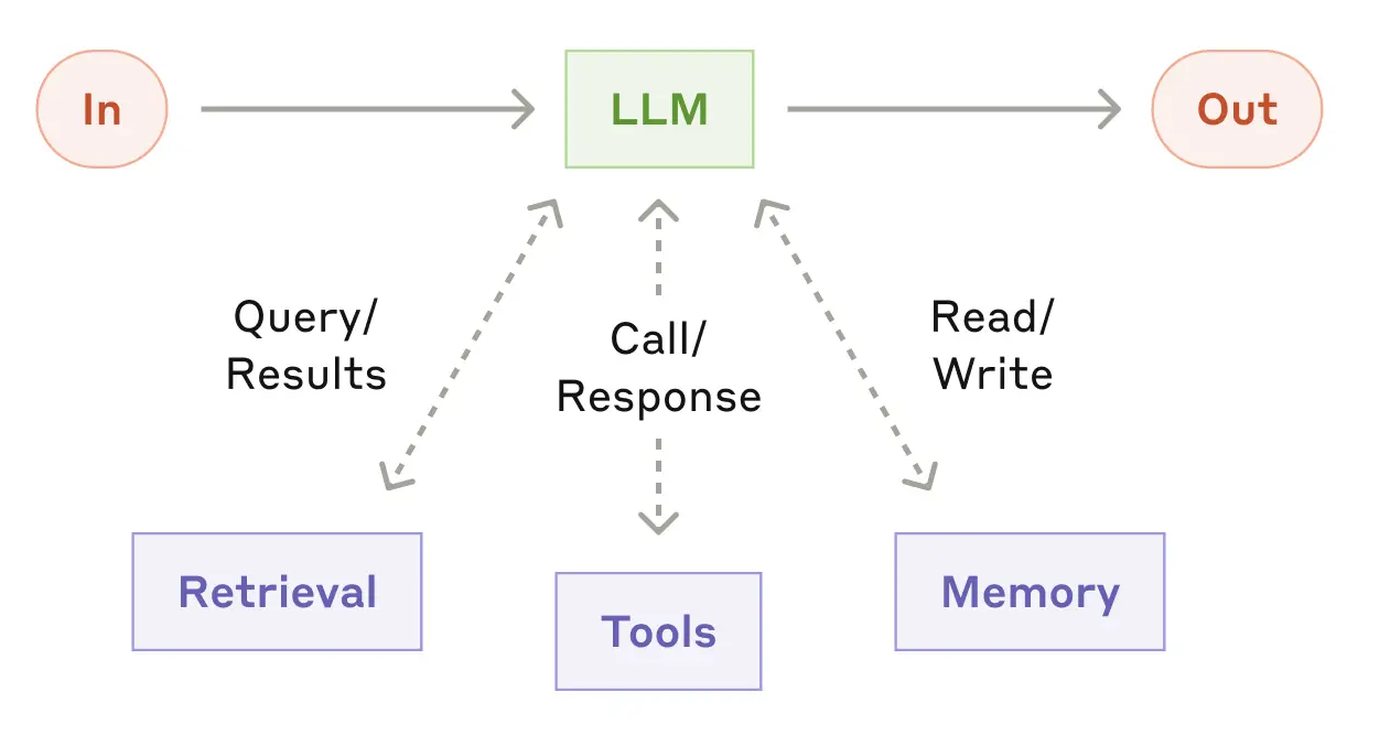
This allows the system to:
- generate follow-up queries
- retrieve additional information
- select tools or skills to perform analysis
- retain and reuse relevant information across steps
Building on this idea, an agentic system is an LLM embedded with tools, memory, and control logic, organized to accomplish tasks in a code-driven manner rather than through a sequence of independent chat interactions.
Important
An LLM becomes truly useful for complex tasks when it is embedded in a system that allows it to act, remember, and iterate, not just respond.
This is the foundation for everything that follows: tools enable action, memory enables persistence, and evaluation enables iteration.
In agentic systems, prompts are no longer one-time interactions.
They become designed components the system can use repeatedly and reliably. The user’s questions shift from:
“What should I ask the LLM right now?”
to “What prompt should this system use every time it performs this task?”
This shift from conversational prompt to designed component is what the progression in Table 19.2 describes.
19.4.2 From Prompts to Functions
To work effectively with LLM APIs, especially when building workflows and agents, we need to move beyond individual prompts and instead convert prompts into functions that are repeatable and structured.
This means explicitly defining in code:
- the inputs
- the instructions and constraints
- the expected type of output
For example:
This makes our prompt now:
- repeatable
- reproducible
- testable
- easier to version (in Git) and refine
- easier to integrate into larger agentic systems
Conceptually, this is the bridge from experimentation to system design:
- Prompts enable experimentation
- Functions provide reusable, callable building blocks
- Workflows organize capabilities into structured processes
- Agents decide which capabilities to use
19.4.3 Workflows
A workflow organizes LLM calls and tools into a predefined sequence of steps.
- The process and control flow are explicitly written in code.
- The sequence of operations is fixed.
- The model fills in details, but does not control the overall structure.
A simple workflow built on the earlier function might look like this:
Here:
generate_code_summary()is a function that encapsulates a prompt to generate code to produce a summary ofmy_data.evaluate_code_summary()is function that checks whether the resulting code is acceptable- the loop defines the workflow
- the control logic is explicit in code
19.4.4 Evaluation
Any time we have a model generate code or an output we want to use, we need to evaluate it before using it in a larger system.
- The evaluation criteria come directly from the constraints you defined in the prompt.
- This is why well-specified constraints matter as much for testing as they do for generation.
The evaluate_code_summary() function performs three conceptual tasks that map to the constraint hierarchy introduced earlier:
- Check execution — does the code run without errors? (Output Goal constraint)
- Validate output structure — is the output the expected type and shape? (Tools / Assumptions constraints)
- Validate output semantics — does the result actually answer the question? (Scope / Output Goal constraints)
A simplified pseudo-code version might look like:
evaluate_code <- function(code, data_context) {

  try:
    output <- execute(code, environment = data_context)
    execution_success <- TRUE
  catch error:
    execution_success <- FALSE
    error_message <- error$message

  if (!execution_success) {
    return(list(
      valid = FALSE,
      feedback = paste("The code failed with error:", error_message)
    ))
  }

  if (!is_expected_type(output)) {
    return(list(
      valid = FALSE,
      feedback = "The output is not in the expected format."
    ))
  }

  if (!passes_reasonableness_checks(output)) {
    return(list(
      valid = FALSE,
      feedback = "The output does not appear to answer the question correctly."
    ))
  }

  return(list(
    valid = TRUE,
    output = output
  ))
}
19.4.5 Agents
While workflows provide structure and reliability, they are limited to predefined sequences of steps.
An agent shifts some of that control to the model itself.
- The model decides which action to take
- The sequence of steps is not fully predetermined
- The system may choose among multiple tools or strategies
A concise working definition:
An agent is a system where the model decides what to do next, rather than following a fixed sequence of steps.
for (i in 1:max_steps) {
  action <- call_model("
    Given the task and current state,
    choose the next action:
    - generate_code_summary
    - plot_data
    - stop
  ")
  if (action == "generate_code_summary") {
    code <- generate_summary_code("nyc311_clean")
    result <- evaluate_code_summary(code)

  } else if (action == "plot_data") {
    plot <- generate_code_plot("nyc311_clean")
    result <- evaluate_code_plot(plot)

  } else if (action == "stop") {
    break
  }
  # model sees results and decides next step
}
The distinction can be summarized as:
- Workflow: we define the process and control flow, and the model fills in the details
- Agent: we define the available functions and tools, and the model helps determine which to use and in what order.
Analogy: Workflows vs Agents and Programming Models
If you are familiar with R Shiny or Dash, it may be helpful to think about workflows and agents in terms of declarative versus reactive programming.
- A workflow is similar to declarative or pipeline-based programming:
- The sequence of steps is explicitly defined
- The control flow is fixed
- Each step executes in a predictable order
- An agent is closer in spirit to reactive systems:
- The next action depends on the current state
- The system adapts dynamically based on intermediate results
- The sequence of operations is not fully predetermined
Note: This is an analogy, not an exact equivalence.
- Reactive systems like Shiny are deterministic and event-driven, while agents rely on probabilistic model outputs to decide what to do next.
- The analogy is useful for intuition about fixed vs dynamic control, but the underlying mechanisms are different.
ImportantWhat an Agent Can Do
An Agent acts by calling functions and tools, the concrete building blocks you define in code and make available to the model.
These building blocks typically take three forms:
- Functions: functions you write that the model can invoke (e.g.,
generate_code_summary()) - Tools: connections to external services or execution environments (e.g., run code, query a database, call an API)
- Skills: reusable packages of instructions and code for recurring tasks.
- These are a more structured form of prompt-based function, used in some platforms including Claude Code.
- The concept is platform-portable even if the specific format varies.
The term capabilities appears frequently in general discussion of LLM systems and means roughly the same thing: what the system is able to do.
- We use the more specific terms here because they correspond directly to things you will write and call in R.
Agents are:
- more flexible
- better suited for open-ended tasks
- capable of adapting based on intermediate results
But they are also:
- harder to debug
- less predictable
- more sensitive to prompt and evaluation design
19.4.6 Choosing Between Workflows and Agents
Many tasks can be handled effectively without using agents.
Well-designed workflows are often:
- easier to implement
- more reliable
- simpler to debug
- sufficient for structured tasks
As with machine learning, increasing flexibility and capability comes with increased complexity and reduced predictability.
Important
The goal is to match the level of system complexity to the problem.
- Use workflows when the task is structured and predictable
- Use agents when the task requires flexibility, adaptation, or decision-making
The concepts introduced here, prompts, functions, workflows, and agents, become easier to understand through working code than through description alone.
The next section introduces ollama, a tool for running LLMs locally on your own machine, and works through examples of each of these components to illustrate how they work and how they fit together in practice.
19.5 Building Workflows with Ollama
Section 19.2 introduced prompt engineering as an interactive practice of writing, refining, and iterating on prompts through a chat interface.
Section 19.3 disucssed developing a more structure approach for code-driven interactions with LLMs.
Section 19.4 introduced the concept of agentic systems as code-driven systems that use LLMs to generate and execute code, evaluate results, and make decisions about next steps.
It is time to move from discussion to practice.
- This section works through concrete examples of calling a model from R, encapsulating prompts as functions, and building workflows that generate, evaluate, and refine code.
To do that we need a way to call a model programmatically from R — and that is where Ollama comes in.
19.5.1 What is Ollama?
Ollama is an open-source tool that allows you to download and run large language models locally on your own machine.
Ollama provides:
- a model library with a growing collection of open-source LLMs that can be downloaded with a single terminal command
- a local server that runs as a background process and exposes a simple HTTP API for sending prompts and receiving responses
- a command-line interface for managing models, checking status, and testing prompts interactively in the terminal
When Ollama is running it behaves like a local version of a cloud API — your R code sends a prompt over HTTP to localhost and receives a response exactly as it would with a cloud provider, but without leaving your machine.
This makes Ollama a practical environment for exploring LLMs and building workflows for several reasons:
- No API key or account required: models run entirely on your local machine, so you can experiment immediately without setting up credentials or worrying about usage costs
- Full visibility into requests and responses: because you control the HTTP call directly, you can see exactly what is sent to the model and what comes back, which makes it easier to understand and debug the prompt-response cycle
- Multiple models available locally: you can pull and compare different models with a single terminal command, making it straightforward to observe how model size, training focus, and architecture affect output quality for the same prompt
- Fast iteration: local inference avoids network latency and rate limits, so the edit-run-evaluate loop is faster during development and the workflow concepts are not obscured by waiting for API responses
- Direct transfer to cloud APIs: the same prompt functions, evaluation logic, and workflow patterns work with cloud APIs such as Anthropic or OpenAI by swapping the calling function, e.g.,
call_ollama(), for a different model interface function; the rest of the system stays unchanged
19.5.2 Using Ollama from R
To install Ollama see the Install Ollama appendix (Appendix C) or go to <https://ollama.com>>.
Use the terminal to “pull” at least two models
llama3.2for lightweight general prompting -ollama pull llama3.2:1bqwen2.5-coder:3bfor coding tasks -ollama pull qwen2.5-coder:3b
We can now use these models to illustrate several concepts
- Use interactive prompts to compare outputs across models
- Encapsulate prompts into functions
- Build a simple workflow
- Create an agentic system
19.5.2.1 Starting and Verifying Ollama
Before using Ollama from R, ensure the local ollama service is running.
- On MacOS or Windows, launching the Ollama application will start the background service.
- You can also start it from the terminal:
You should get output similar to
[GIN] 2026/04/04 - 10:50:21 | 200 | 274.5µs | 127.0.0.1 | GET "/api/version"To check the installed models, use the terminal with
You should get output similar to the following but based on the models you installed.
AME                ID              SIZE      MODIFIED
qwen2.5-coder:3b    f72c60cabf62    1.9 GB    23 hours ago
qwen2.5-coder:7b    dae161e27b0e    4.7 GB    23 hours ago
llama3.2:latest     a80c4f17acd5    2.0 GB    14 months ago
To check it is configured properly, test a model in the terminal.
Your terminal cursor should change to a blinking prompt and you can type a question to the model.
- For example: describe data science in one sentence?
- You may get a response similar to the following:
>>> describe data science in one sentence
Data science is the process of extracting insights, knowledge, and value from
data, using a combination of mathematical and computational techniques, such as
machine learning, statistics, and programming, to inform business decisions,
solve complex problems, or answer strategic questions.- To stop the current model use CTRL D in the terminal, or, if you are using the Ollama app, click the “Stop” button.
Ollama supports interactive chat in the terminal but we want to interact with Ollama through R, and we will see how to do that in the next section.
19.5.2.2 Calling Ollama from R
We access the model using a function call over HTTP using the {httr2} package.
- By default, Ollama runs on
http://localhost:11434.
Let’s define a function to call the model, with arguments for the prompt and the model of choice, and then parse the JSON response and return the response element.
- The function creates and sends a {httr2} request to the Ollama
/api/generateendpoint.
req_body_json()creates structured input for the model- model: the model to run
- prompt: the task or question
- stream: controls how results are returned
stream = FALSEmeans don;t stream the results; wait for the model to finish the full response before returning it so the return is one JSON object thatresp_body_json()can handle.
Now let’s use the function to send a prompt to the model.
[1] "A workflow refers to a series of steps or processes defined and executed for completing a specific task or goal."We can send the same prompt to different models and compare the results.
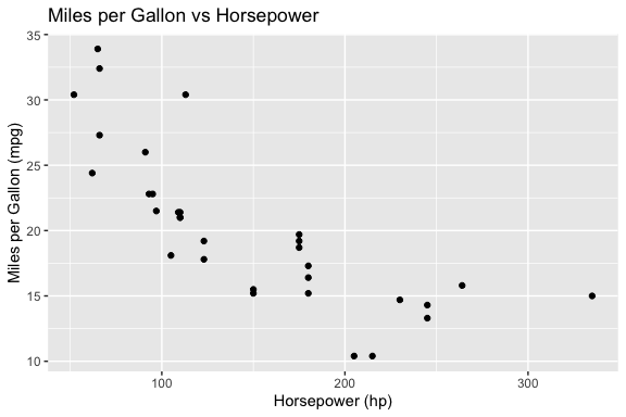
[1] "Here is a simple R code that uses ggplot2 to create a scatter plot of MPG vs HP from the built-in 'mtcars' dataset:\n\n```r\n# Load necessary libraries\nlibrary(ggplot2)\n\n# Create the scatter plot\nggplot(mtcars, aes(x = hp, y = mpg)) +\n geom_point() +\n labs(title = \"Scatter Plot of MPG vs HP\",\n subtitle = \"From the mtcars dataset\",\n x = \"Horsepower\",\n y = \"Miles per Gallon\")\n```\n\nIn this code:\n\n- We first load the ggplot2 library.\n- Then, we use `ggplot()` to create a new ggplot object, passing in the 'mtcars' dataset and specifying that 'hp' should be on the x-axis ('x') and 'mpg' should be on the y-axis ('y').\n- The `geom_point()` function is used to add points to the plot for each observation in the data.\n- Finally, we use the `labs()` function to set labels for the title, subtitle, x-axis, and y-axis of the plot."[1] "Certainly! Below is an example of how you can use the `ggplot2` package in R to plot `mpg` (miles per gallon) against `hp` (horsepower) from the `mtcars` dataset.\n\n```r\n# Load the ggplot2 package\nlibrary(ggplot2)\n\n# Create a scatter plot\nggplot(mtcars, aes(x = hp, y = mpg)) +\n geom_point() +\n labs(title = \"Miles per Gallon vs Horsepower\",\n x = \"Horsepower (hp)\",\n y = \"Miles per Gallon (mpg)\") +\n theme_minimal()\n```\n\nThis code will generate a scatter plot with `hp` on the x-axis and `mpg` on the y-axis. The `geom_point()` function is used to create the points, and `labs()` is used to add titles and labels to the axes and the plot. The `theme_minimal()` function sets a clean and minimalist theme for the plot."[1] "Sure! Below is an example of R code that uses `ggplot2` to create a scatter plot showing the relationship between miles per gallon (`mpg`) and horsepower (`hp`) from the `mtcars` dataset.\n\nFirst, make sure you have `ggplot2` installed. If not, you can install it using the following command:\n\n```R\ninstall.packages(\"ggplot2\")\n```\n\nThen, load the necessary libraries and create the plot:\n\n```R\n# Load the required library\nlibrary(ggplot2)\n\n# Create a scatter plot of mpg vs hp from mtcars\nggplot(mtcars, aes(x = hp, y = mpg)) +\n geom_point() +\n labs(title = \"MPG vs HP\",\n x = \"Horsepower (hp)\",\n y = \"Miles per Gallon (mpg)\") +\n theme_minimal()\n```\n\nThis code will generate a scatter plot with horsepower on the x-axis and miles per gallon on the y-axis. The `theme_minimal()` function is used to apply a clean, minimalistic theme to the plot.\n\nYou can customize the plot further by adding additional layers or modifying the appearance using various `ggplot2` functions."- Oops! the models return formatted text, not tidyverse style code we want.
This is what models do, they return text.
LLMs don’t return answers; they return text that must be interpreted.
The text in a response may include:
- explanatory text
- formatting characters such as
\nfor new lines. - markdown code fences
- comments
- installation commands we do not want to run
To compare models more clearly, it is helpful to extract just the code portion of the response.
19.5.3 Extracting Code from Model Responses
Let’s create a function to extract code from the response and name it extract_code().
We want the function to:
- Extract the code chunks
- Remove code fences and formatting characters
- Replace the escaped new line characters with actual new lines.
Now extract the code from the responses
[1] "# Load necessary libraries\nlibrary(ggplot2)\n\n# Create the scatter plot\nggplot(mtcars, aes(x = hp, y = mpg)) +\n geom_point() +\n labs(title = \"Scatter Plot of MPG vs HP\",\n subtitle = \"From the mtcars dataset\",\n x = \"Horsepower\",\n y = \"Miles per Gallon\")\n"[1] "# Load the ggplot2 package\nlibrary(ggplot2)\n\n# Create a scatter plot\nggplot(mtcars, aes(x = hp, y = mpg)) +\n geom_point() +\n labs(title = \"Miles per Gallon vs Horsepower\",\n x = \"Horsepower (hp)\",\n y = \"Miles per Gallon (mpg)\") +\n theme_minimal()\n"[1] "install.packages(\"ggplot2\")\n"We now have the code from each model as a string. We can use base R functions to view it and execute it.
cat()is useful to view the code with proper formatting and new lines.eval(parse())allows us to execute the code as R code.
Let’s compare all three.
llama code
 # Load necessary libraries
library(ggplot2)

# Create the scatter plot
ggplot(mtcars, aes(x = hp, y = mpg)) +
  geom_point() +
  labs(title = "Scatter Plot of MPG vs HP",
       subtitle = "From the mtcars dataset",
       x = "Horsepower",
       y = "Miles per Gallon")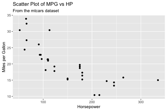
qwen3b code
 # Load the ggplot2 package
library(ggplot2)

# Create a scatter plot
ggplot(mtcars, aes(x = hp, y = mpg)) +
  geom_point() +
  labs(title = "Miles per Gallon vs Horsepower",
       x = "Horsepower (hp)",
       y = "Miles per Gallon (mpg)") +
  theme_minimal()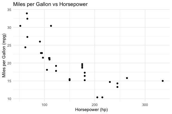
qwen7b code
install.packages("ggplot2")The following package(s) will be installed:
- ggplot2 [4.0.3]
These packages will be installed into "~/Courses/DATA-413-613/lectures_book/renv/library/macos/R-4.5/aarch64-apple-darwin20".
# Installing packages --------------------------------------------------------
[32m✔[0m ggplot2 4.0.3 [linked from cache]
Successfully installed 1 package in 4.9 milliseconds.Interpretation of results
- Did the models all return usable code?
- Which model produces the best code?
- Which is fastest?
- Which requires the least editing?
This illustrates a key idea: Model selection is part of system design.
ImportantHandling Variability in Model Output
When working with LLMs, you must be prepared for inconsistent response structure.
The extract_code() function works well when the model returns a single code block, however,
- Repeating the same prompt may produce responses with multiple code blocks
extract_code()only extracts the first block, which may not be the one you want to run
This highlights an important principle:
Workflows should be designed for the range of outputs a model may produce, not just a single observed response.
To handle this variability, we can extract all code blocks with str_extract_all() and then decide which one(s) to use.
This approach makes the workflow more robust by separating:
- extraction (get all candidate code)
- selection (decide what to run)
In more advanced systems, this selection step may itself become part of the evaluation process.
19.5.4 Encapsulating Prompts in Functions
Instead of repeatedly writing prompts, we now encapsulate them in a function that takes parameters and generates the appropriate prompt as in Listing 19.7.
- This is a thin wrapper function we will expand later.
- The default model is
qwen2.5-coder:3b, a model trained for code-generation, that balances output quality with response speed for local use.- The 7B version produces better results but is noticeably slower, which matters when rendering a document or iterating quickly.
- This is a common trade off in system design: a faster, smaller model is often the right default for development and experimentation, with a larger model reserved for final runs or tasks where quality is critical.
Now we can reuse our prompts, get the response, extract the code, and evaluate if the response included code.
- Keeping the model response separate from the code extraction and execution at first allows for easier debugging and validation of the model output before running it.
Once you are satisfied the responses are consistent, you can wrap the two functions in a single function that generates the code and executes it.
ImportantContext-limited Responses.
This code may get a plot of mpg vs hp from the mtcars dataset or it may generate a prompt in the console to install {ggplot2} as the model wanted to ensure the packages were installed.
This is an example of a context-limited response: the model is trying to be helpful by ensuring the system has the necessary packages, but that is creating an interactive step which is not what we want in this case, especially if we want to render the file.
There are several option to handle this but the first step is to give the model more context and we do that by adding more constraints to our prompt.
Let’s refine the prompt to add a role and more constraints
my_prompt <- paste(
  "You are a coding assistant working in R.",
  "Write R code using ggplot2 to plot hp vs mpg from mtcars.",
  "Assume all required packages are already installed.",
  "Do NOT include install.packages().",
  "Use library() only if needed.",
  "Return exactly one fenced R code block.",
  "Use at least one geom to plot the points."
)
The role assignment, “You are a coding assistant working in R”, signals to the model that it should prioritize concise, executable code over explanation or installation instructions.
- This is the same role concept introduced in Table 19.1, now applied as a concrete line in a prompt.
However, adding this line manually to every prompt is error-prone and inconsistent.
- A better approach is to make the role a parameter or argument of the
get_model_response()function itself (Listing 19.7).- Choose a default for the role that is appropriate for many tasks.
- In this case, “You are a coding assistant working in R.” is a good role for many of our tasks.
- You may also get an error due to incomplete code in the response, e.g., missing a closing parenthesis.
To make the code more robust, the next step is to add error checking into the code.
- We can use
tryCatch()to handle cases where the model response is not as expected and generates an error condition.
Let’s create a safe_execute() function to wrap the code in a tryCatch() block that returns a list with success status and either the result or the error message.
Now update generate_and_run_plot() from Listing 19.8 to use safe_execute() to run the code.
- The function in Listing 19.10 returns a structured result that
- includes success status,
- the generated code (if successful),
- the result of execution with any error message.
generate_and_run_plot <- function(prompt, model = "qwen2.5-coder:3b") {

  response <- get_model_response(prompt, model)
  code <- extract_code(response)

  if (is.null(code)) {
    return(list(success = FALSE, error = "No code extracted"))
  }

  exec <- safe_execute(code)

  # for interactive use, check if execution was successful and print error if not
  if (!exec$success) {
    cat("Execution failed:\n", exec$error, "\n")
  }

  return(list(
    success = exec$success,
    code = code,
    result = if (!is.null(exec$result)) exec$result else NULL,
    error  = if (!is.null(exec$error)) exec$error else NULL
  ))
}
Now when we run the function, we get a structured output that indicates whether the code execution was successful, the generated code if successful, and any error messages if it failed.
$success
[1] TRUE

$code
[1] "# Load the ggplot2 package\nlibrary(ggplot2)\n\n# Create a scatter plot of hp vs mpg from mtcars dataset\nggplot(mtcars, aes(x = hp, y = mpg)) +\n  geom_point() +\n  labs(title = \"Scatter Plot: Horsepower vs Miles per Gallon\",\n       x = \"Horsepower (hp)\",\n       y = \"Miles per Gallon (mpg)\")\n"

$result

$error
NULL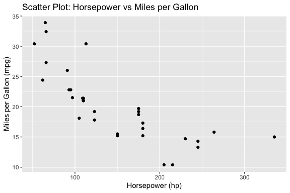
NoteUsing tryCatch() for Workflow Robustness
When running code generated by a model, errors are common and should be expected.
The tryCatch() function allows us to run code without stopping execution if an error occurs.
- Instead of crashing, the error is captured and returned as information the system can use.
The tryCatch() function wraps an expression and monitors its execution.
- It attempts to run the code inside the main block
- If the code completes normally, the result is returned
- If an error occurs, execution is interrupted, and control is passed to the error handler
In python, the (try / except) block serves a similar purpose, allowing you to handle exceptions gracefully without crashing the program.
try:
    result = eval(code)
    output = {"success": True, "result": result}
except Exception as e:
    output = {"success": False, "error": str(e)}
Conceptually, this creates two possible paths:
- Success path: code runs and returns a result
- Error path: the code fails, and the error handler captures the condition and returns structured information
In this sense, tryCatch() turns execution into a controlled branching process. As shown in Listing 19.9, instead of letting an error terminate execution, tryCatch():
- intercepts the error condition
- extracts relevant information (e.g., the message)
- returns it as part of a structured output
This enables a more robust workflow:
- The code can be attempted safely
- Errors can be inspected and reported
- The system can decide what to do next (e.g., revise the prompt or try again)
Using tryCatch() converts an code-stopping error into a structured output that can be used to inform the next steps in the workflow.
This pattern is critical in workflows and agentic systems because:
- it allows the system to continue running
- it makes errors observable and usable
- it enables decisions such as retrying, revising prompts, or selecting a different action
tryCatch() does not prevent errors, it makes them part of the system’s output that can be evaluated by humans or by code.
19.5.5 Workflows
Up to this point, we have focused on building individual components.
We now combine them into workflows, the fixed, code-controlled sequences described in Table 19.2.
19.5.5.1 Workflow 1: Generate -> Execute -> Evaluate (baseline loop)
This is Listing 19.9 converted into a workflow pattern.
- This is a baseline workflow where the control flow is fixed and defined entirely in code and we get results (plot or error) that can be evaluated.
run_once <- function(prompt, model = "qwen2.5-coder:3b") {
  response <- get_model_response(prompt, model)
  code <- extract_code(response)

  if (is.null(code)) {
    return(list(
      success = FALSE,
      code = NULL,
      result = NULL,
      error = "No code extracted"
    ))
  }

  exec <- safe_execute(code)

  return(list(
    success = exec$success,
    code = code,
    result = if (!is.null(exec$result)) exec$result else NULL,
    error  = if (!is.null(exec$error)) exec$error else NULL
  ))
}
run_once(my_prompt)
$success
[1] TRUE
$code
[1] "library(ggplot2)\n\nggplot(mtcars, aes(x = hp, y = mpg)) +\n geom_point()\n"
$result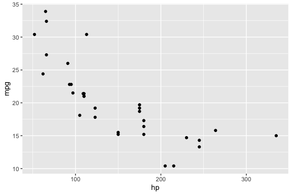
$error
NULL- Note: we removed the interactive feedback for humans to keeps the functions clean for workflows and agents, but it also means we won’t see the error in the console if it occurs.
- If we want, we can add it back in the console to see the error if it occurs.
19.5.5.2 Workflow 2: Generate -> Evaluate -> Revise using an iterative loop
This workflow introduces feedback and iteration by combining functions that perform computation (e.g., model calls, code execution) with flow-control structures such as loops.
- The loop provides a natural way to track progress across attempts and observe how the workflow evolves over time.
- When designing workflows, remember that functions return results; workflows manage and monitor the process.
Listing 19.12 is a basic “Generate -> Evaluate -> Revise” loop that allows the system to attempt a task multiple times.
- If there is an error, the workflow refines the prompt by adding the task to fix the error (message) from the unsuccessful attempt.
run_with_retry()subsumesrun_once()since settingmax_attempts = 1is equivalent.
run_with_retry <- function(prompt, model = "qwen2.5-coder:3b",
                           max_attempts = 3) {

  for (i in 1:max_attempts) {

    cat("Attempt:", i, "\n")

    response <- get_model_response(prompt, model)
    code <- extract_code(response)

    if (is.null(code)) {
      next
    }

    exec <- safe_execute(code)

    if (exec$success) {
      return(list(success = TRUE, code = code))
    }

    # simple refinement strategy
    prompt <- paste(
      prompt,
      "\nFix the error:",
      exec$error
    )
  }

  return(list(success = FALSE, error = "Max attempts reached"))
}- It’s good practice to avoid printing messages inside functions to keep them reusable and composable.
- However, it is appropriate to use
cat()messages as part of the flow control within the workflow to log progress.- In agentic systems, using logging to track the flow is important because the sequence of actions is not fixed.
- In more complex systems, logging data is often written to files rather than printed to the console, allowing results to be stored, analyzed, and reused across runs.
This simple workflow works, but exposes limitations that motivate a more structured approach for the workflow:
- the prompt keeps growing and becoming noisy as the same error message may get added over and over
- missing code is not handled well
- constraints may be lost over iterations
- evaluation is minimal (only execution success)
We can improve the workflow by making the evaluation and refinement steps more explicit.
19.5.5.3 A Refined Workflow 2: Generate -> Evaluate -> Revise
So far, evaluation has been minimal: the workflow only checks whether the generated code can be extracted and executed.
- In practice, that is often not enough.
A stronger evaluation strategy separates at least three kinds of checks in addition to Execution checks:
- Structure checks: ensure the code contains expected building blocks or elements.
- Task-specific checks: require you to know specific elements of the prompt, e.g., the data set or variables, to ensure the code appears to satisfy the specific analytical goal.
- Process Constraints: enforce workflow rules (e.g., disallow install.packages()).
For example, for a plotting task, these can be distinguished as follows:
- Structure checks: These ensure the code has the basic elements of a plot.
- does the code contain “ggplot(”?
- does it include at least one “geom_ layer”?
- Task-specific checks: These ensure the code is actually trying to solve the intended task, not just producing some plot.
- are the correct variables used (e.g., hp and mpg)?
- are they mapped to the correct axes?
- Process Constraints These enforce workflow constraints, not the task itself.
- does the code avoid “install.packages(”?
These try to ensure the code is actually solving the intended task, not just producing some plot.
Note
Task-specific checks require some explicit representation of what the prompt is asking for.
- If the prompt remains fully flexible, then task-specific evaluation must also remain relatively general.
One way to support stronger evaluation later is to include two parts to the prompt:
- the prompt text used for generation which can be free text
- a structured set of expected elements to be used for validation e.g.,
expected = list(
    dataset = "mtcars",
    variables = c("hp", "mpg"),
    required = c("ggplot", "geom_"),
    forbidden = c("install.packages")
  )
This allows the workflow to remain flexible while still supporting more targeted evaluation based on structured data in the prompt.
In this example, the prompt is still a flexible argument so task-specific evaluation is limited.
- It is more practical now to focus on structure, constraint, and execution checks.
- More specific evaluation becomes possible when the system has explicit expectations about the task, such as keywords, variables, datasets, or required output elements.
Let’s encapsulate the structure and process checks in a function as in Listing 19.13.
evaluate_plot_code_structure <- function(code) {
  checks <- list(
    has_ggplot = stringr::str_detect(code, "ggplot\\("),
    has_geom = stringr::str_detect(code, "geom_"),
    installs_packages = stringr::str_detect(code, "install\\.packages\\s*\\(")
  )
  list(
    success = checks$has_ggplot && checks$has_geom && !checks$installs_packages,
    checks = checks
  )
}
We can use the evaluate_plot_code_structure() function to make the workflow more robust by no longer treating every executable result as a successful result for our task.
Listing 19.14 shows a refined workflow that makes the stages clear and uses a better evaluation and prompt refinement strategy.
- This version now separates two kinds of failure:
- evaluation failure: the code does not meet the expected structure or task constraints
- execution failure: the code looks reasonable but still does not run
run_with_retry <- function(prompt,
                           model = "qwen2.5-coder:3b",
                           max_attempts = 3) {
  original_prompt <- prompt
  last_error <- NULL
  last_code <- NULL
  last_checks <- NULL

  for (i in 1:max_attempts) {
    cat("Attempt:", i, "\n")

    # Step 1: generate a response from the model
    response <- get_model_response(prompt, model)

    # Step 2: extract code from the response
    code <- extract_code(response)
    last_code <- code

    # Step 3: handle missing code explicitly
    # If no fenced R code block was extracted, we refine the prompt by asking for exactly one code block.
    if (is.null(code)) {
      last_error <- "No executable code block was extracted from the response."

      prompt <- paste(
        original_prompt,
        "\nThe previous response did not contain a usable R code block.",
        "Return exactly one fenced R code block.",
        "Do not include explanation."
      )

      next
    }

    # Step 4: evaluate the code before execution
    # Evaluate structure/process constraints: 'ggplot()', 'geom_', and no 'install.packages()'.
    eval_result <- evaluate_plot_code_structure(code)
    # Preserve checks from last evaluation attempt for the failure return at the end of the function
    last_checks <- eval_result$checks

    # Step 5: if structure/process checks fail, refine the prompt accordingly
    # If any structure/process conditions are violated, we build a message explaining what was wrong
    # and use it to refine the prompt. This helps the model correct the specific problem.
    if (!eval_result$success) {
      refinement_messages <- c()

      # 'ggplot()' missing: structure problem.
      if (!eval_result$checks$has_ggplot) {
        refinement_messages <- c(
          refinement_messages,
          "The previous code did not include ggplot()."
        )
      }

      # No geom_ layer: structure problem.
      if (!eval_result$checks$has_geom) {
        refinement_messages <- c(
          refinement_messages,
          "The previous code did not include a geom_ layer such as geom_point()."
        )
      }

      # install.packages() found: process constraint problem.
      if (eval_result$checks$installs_packages) {
        refinement_messages <- c(
          refinement_messages,
          "The previous code included install.packages(), which should not be used."
        )
      }

      last_error <- paste(refinement_messages, collapse = " ")

      prompt <- paste(
        original_prompt,
        "\nRevise the code to address the following problems:",
        last_error,
        "Assume required packages are already installed.",
        "Do not include install.packages().",
        "Return exactly one fenced R code block and no explanation."
      )

      next
    }

    # Step 6: execute the code safely only after evaluation passes
    exec <- safe_execute(code)

    # Step 7: if execution succeeds, return a structured result
    # At this point, the code passed structure and process checks and ran without error.
    if (exec$success) {
      return(list(
        success = TRUE,
        attempts = i,
        prompt = prompt,
        code = code,
        checks = eval_result$checks,
        result = if (!is.null(exec$result)) exec$result else NULL,
        error = NULL
      ))
    }

    # Step 8: if execution fails, store the error and refine the prompt
    # Execution failure means the code looked reasonable but raised a runtime error.
    # We include that error in the prompt so the model can fix it in the next iteration.
    last_error <- exec$error

    prompt <- paste(
      original_prompt,
      "\nThe previous code passed the structural checks but failed with this execution error:",
      last_error,
      "Revise the code so that it runs successfully.",
      "Assume required packages are already installed.",
      "Do not include install.packages().",
      "Return exactly one fenced R code block and no explanation."
    )
  }

  # Step 9: if all attempts fail, return the final state
  # We return failure state with the last prompt, last code, checks, and error.
  return(list(
    success = FALSE,
    attempts = max_attempts,
    prompt = prompt,
    code = last_code,
    checks = last_checks,
    result = NULL,
    error = paste("Max attempts reached.", last_error)
  ))
}- The evaluation step in Listing 19.14 uses deterministic code-based checks.
- We will see later how the model itself can take on the evaluator role, which is where role as a function parameter becomes important at the workflow level.
Note
As you’ve seen, even a relatively simple plotting task requires a lot of code once you handle extraction, evaluation, and refinement and include error handling.
- Converting prompts into functions and structuring them into workflows keeps this complexity manageable.
- It also makes your code reusable, testable, and easier to extend or debug.
- This approach is key as tasks grow beyond simple demonstrations.
We will extend this pattern to create an agent, replacing the fixed control flow with model-driven decisions about what to do next.
19.6 From Workflows to Agents
In the workflow section Section 19.5.5, we defined the process and control flow explicitly in code: generate, evaluate, revise, repeat.
- The model filled in details but did not decide what to do next.
An agent inverts that relationship.
- We define the available tools (the actions the system can take), and the model decides which to use and in what order, based on the current task and state.
This section builds that progression in three steps:
- Define a set of tools the agent can call
- Build a simple agent where the model chooses among them
- Refine toward a balanced design that combines model flexibility with structured evaluation
As these systems grow, a new challenge emerges: managing what information goes into each model call. We will return to that challenge, known as context engineering, once the basic agent structure is working.
19.6.1 Defining Functions and Tools
Tools are implemented as functions in R (or Python, JavaScript, or any other language).
The distinction is one of perspective:
- you write and call functions in your code;
- the model invokes them as tools.
When a function is registered with an agent so the model can invoke it, it becomes a tool.
Functions available to an agent fall into three categories:
| Function type | What it does | Example |
|---|---|---|
| Deterministic function | Wraps existing code, produces predictable output | plot_mpg_hp() |
| Prompt-based generation function | Sends a prompt, returns model output | generate_code_scatterplot() |
| Prompt-based evaluation function | Sends output back to model for assessment | evaluate_with_model() |
Evaluation is always a separate step from generation and can itself take two forms:
- Code-based evaluation: R functions that inspect output directly using pattern matching, execution checks, or structural tests — as in
evaluate_code_scatterplot(). - Prompt-based evaluation: a second model call that asks the model to assess the output, typically using a reviewer or evaluator role rather than a coding assistant role
The examples in this section use code-based evaluation because it is deterministic, fast, and does not consume additional model calls.
- Prompt-based evaluation becomes useful when the criteria for correctness are difficult to express as code
- for example, assessing whether a summary captures the right information or whether generated code follows a style guide.
Below are two deterministic functions for summarizing data and plotting MPG vs HP, along with a prompt-based generation function to generate code for making a plot.
# Deterministic function: summarize mtcars dataset
summarize_dataset <- function(df) {
  df %>%
    summarise(across(everything(), mean, na.rm = TRUE))
}

# Deterministic function: plot mpg vs hp using ggplot2
plot_mpg_hp <- function(df) {
  df  |>
    ggplot(aes(x = hp, y = mpg)) +
    geom_point() +
    labs(
      title = "MPG vs HP",
      x = "Horsepower",
      y = "Miles Per Gallon"
    ) +
    theme_minimal()
}

# Prompt-based function: generate ggplot code via LLM
generate_plot_code <- function(prompt, model = "qwen2.5-coder:3b") {
  call_ollama(prompt, model)
}
19.6.2 A Simple Agent
When building an agent, we define the available tools; the model decides which to call and in what order based on the task description.
- The control flow is no longer fixed as the model participates in determining the process at runtime.
The agent in Listing 19.16 has three key characteristics:
- Functions as actions: each available action is implemented as a named function with a clear purpose
- Model-driven control flow: a helper function prompts the model to choose the next action rather than following a fixed sequence
- Bounded iteration: the loop runs until the model selects “stop” or max_steps is reached, preventing runaway execution
# Prompt the model to choose an action based on a task description
choose_action <- function(task_description, model = "qwen2.5-coder:3b") {
  # The prompt lists available actions; the model must respond with one
  call_ollama(
    paste(
      "You are an agent that can perform the following actions:",
      "- summarize: Summarize the mtcars dataset.",
      "- plot: Create a plot of mpg vs hp.",
      "- stop: Indicate that the task is complete.",
      "",
      "Task:", task_description,
      "",
      "Choose exactly one action (summarize, plot, or stop) and return only that word.",
      sep = "\n"
    ),
    model
  )
}

# Agent loop that calls the chosen function
run_agent <- function(task_description,
                      data = mtcars,
                      model = "qwen2.5-coder:3b",
                      max_steps = 5) {

  for (i in 1:max_steps) {
    cat("Agent step:", i, "\n")

    action <- trimws(choose_action(task_description, model))

    # If the model says "summarize", call the summarization function
    if (grepl("^summarize", action, ignore.case = TRUE)) {
      summary_result <- summarize_dataset(data)
      print(summary_result)
    }
    # If the model says "plot", call the plotting function
    else if (grepl("^plot", action, ignore.case = TRUE)) {
      # In a real system, you might display the plot to the user.
      plot_mpg_hp(data)
    }
    # If the model says "stop", break the loop
    else if (grepl("^stop", action, ignore.case = TRUE)) {
      cat("Agent has determined the task is complete.\n")
      break
    }
    # If an unexpected action is returned, notify and exit
    else {
      cat("Unrecognized action:", action, "\n")
      break
    }
  }

  invisible(NULL)
}
In this simple agent the model decides which tool to invoke at each step.
- The functions (
summarize_dataset()andplot_mpg_hp()) are deterministic: once the model selects an action, the outcome is fully predictable. - The model contributes only the routing decision, not the result.
- The loop stops when the model chooses stop or when it reaches max_steps.
This pattern illustrates the core idea of an agent:
We define the available tools; the model helps determine the process by choosing actions at runtime.
19.7 Considerations for Designing an Agent
The simple agent in Listing 19.16 is a starting point, but want to refine it to be more comprehensive and robust.
To do that we’ll explore a few considerations about designing and building an Agent that refines the simple agent while allowing for exploration, reuse, and extension.
19.7.1 Design to Balance Flexibility and Specificity
Refining agentic systems involves balancing flexibility and specificity, both in how you write prompts and how you structure tools.
- Flexibility: letting the LLM interpret open‑ended instructions and decide how to implement them to minimize your effort.
- Specificity adding constraints that drive the LLM to choose among a set of well‑defined tools or prompts that get you the results you want.
Both approaches have pros and cons and thus tradeoffs
Leveraging the LLM’s Flexibility
- Pros:
- You can describe tasks in natural language and let the model decide how to solve them.
- Flexibility enables the LLM to exploration or experiment and can surface alternative approaches you may not have considered or know about.
- Cons:
- Outputs may be inconsistent, incorrect, or use disallowed patterns. -This often leads to iterative refinement and requires strong evaluation and error handling.
Using Specific Tools
- Pros:
- Defining reusable functions or prompt templates creates predictable, testable behavior.
- Evaluation is simpler because each tool has a clear contract.
- Defining reusable functions or prompt templates creates predictable, testable behavior.
- Cons:
- Requires more upfront effort and reduces flexibility.
- Over-specified prompts can be brittle, hard to maintain, with limited reuse across tasks.
- New tasks may require adding new capabilities.
Most effective agentic systems combine both approaches:
- They use flexible prompts to describe broader tasks and the target behavior.
- They use specific tools with evaluation to define and enforce what is acceptable.
Finding this balance and refining it over time is what makes systems both robust and adaptable.
TipFinding the “Goldilocks Zone”
Anthropic recommends using iteration to find a balance of flexibility and specificity. (Anthropic Engineering 2025)
The goal is to:
- Be flexible enough to allow multiple innovative solutions
- LLMs may find creative solutions, but they need enough flexibility to do so.
- New packages, methods, functions, or standards could make a more effective solution.
- Be specific enough to signal what correct output looks like
- Keep complex logic in code and evaluation, not buried in prompts
Start Flexible, Then Refine
In practice, you rarely know the all the exact constraints you will want at first.
- Begin with prompts that allow exploration so the model can reveal possible solution paths
- Use evaluation to identify errors, inconsistencies, or undesirable patterns
- Iteratively refine prompts and constraints based on what you observe
Prompt design is iterative: exploration first, precision later.
19.7.2 Three Examples of Agent Designs: A Spectrum
The following three (illustrative) agent designs span the spectrum from fully-flexible to highly-specific, plus an intermediate balanced version.
- In each case the LLM participates, but the amount of scaffolding and control you provide varies.
19.7.2.1 A High‑Flexibility Agent
Example task: “Explore the penguins data set. Summarize the key variables and create a plot that shows an interesting relationship.”
How it works:
- The agent passes the entire request to the LLM with very little constraint.
- The model decides which summary statistics to compute and which variables to plot (scatter, box, or something else). It generates R code for both.
- The agent extracts the code and executes it, then evaluates whether it ran successfully.
- If the code fails or the result is unsatisfactory, the agent asks the model to revise the code based on the error message and tries again.
Trade‑offs: This leverages the LLM’s creativity but often requires multiple iterations. The model might choose a plot type or variables you didn’t intend, and your evaluation logic has to handle many possible outputs.
19.7.2.2 A High‑Specificity Agent
Example task: “Summarize the penguins data frame and plot bill length versus bill depth.”
How it works:
- You define specific, deterministic functions ahead of time, such as:
summarize_df(df): computes means and standard deviations for all numeric columns.plot_scatter(df, x_var, y_var): produces a ggplot2 scatter plot for a data frame and two columns with associated labels.
- The agent’s prompt tells the model only what functions are available (“summarize” or “plot”), and the model chooses which to invoke in order (e.g., summarize first, then plot).
- The agent runs the chosen function directly, no code generation, and returns the result.
Trade‑offs: This is reliable and fast, because everything is predefined. But it’s also rigid: if you want a box plot, violin plot, or different summary statistics, you’ll need to add a new function and expose it to the model.
19.7.2.3 A Balanced Agent with Generic Prompt‑Based Capabilities
Example task: “Summarize the penguins data frame and include a plot of bill length versus bill depth.”
How it works:
- You define generic prompt templates as functions:
generate_code_summarize_df(df_name): ask the model to write R code that summarizes numeric columns using mean and standard deviation, returning only executable code.generate_code_scatterplot(df_name, x_var, y_var): ask the model to write a ggplot2 scatter plot for specified columns with proper labels, returning only executable code.generate_code_boxplot(df_name, num_var, cat_var): ask the model to write a ggplot2 box plot.
- The agent’s decision logic (in choose_action) knows these three functions exist. It asks the model whether to “summarize”, “scatter”, “box”, or “stop”.
- When the model selects an action, the agent calls the corresponding prompt‑based code generation function, extracts and runs the code, and checks that it meets structural constraints (e.g., contains ggplot and a geom_ layer and doesn’t include install.packages()).
- If the code fails, the agent refines the prompt using the error message, then retries.
Trade‑offs: This approach retains flexibility, you aren’t writing ggplot code yourself, but it also provides structure through your prompt templates.
- You decide what is important and acceptable and let the model figure out the rest.
- It reduces iteration compared to the fully flexible case, because the model doesn’t have to decide which plot type to generate; it merely fills in the template.
- At the same time, you can use the same generic functions across different datasets by passing the data set name and column names as parameters.
Bottom Line: There’s no free lunch:
- Giving the LLM full flexibility minimizes your coding but increases the likelihood of back‑and‑forth interactions.
- Pre-defining deterministic functions makes the agent reliable and efficient but requires more upfront work and limits flexibility.
- A balanced design with generic code-generation functions with specific templates can offer the best of both worlds by harnessing the LLM’s strengths while keeping control over what gets executed.
19.7.3 Managing Context Across Multiple Calls
The three agent designs in Section 19.7.2 illustrate a progression that goes beyond flexibility and specificity.
Consider what each design puts into its calls to the model:
The high-flexibility agent makes one call that gets everything: the full task description, no structure, no constraints. The model decides what to do with it.
The high-specificity agent makes one call to choose an action, then runs deterministic functions. The model sees very little context because it does not need much.
The balanced agent makes multiple specialized calls:
- one to choose an action,
- one to generate code, and,
- potentially one to evaluate it.
Each call has a different purpose and needs different information.
That last point is the key one, especially with the balanced agent.
As soon as you have multiple model calls in a system, a new question arises that prompt engineering alone is not set up to answer:
What information should be included in each call to a model?
This is what motivates the recent evolution from prompt engineering to context engineering.
- Prompt engineering focuses on how to write effective instructions for a single call.
- Context engineering addresses what information to include across all the calls in a multi-step system, and, just as importantly, what to leave out. (Anthropic Engineering 2025)
The distinction matters because of two properties of LLMs you have already encountered:
- Context rot: performance degrades as the context window fills. More is not always better.
- Statelessness: each call starts fresh. Information from prior calls only reaches the model if you explicitly include it.
In a multi-call agent, this means you are making active decisions at every step:
- Does the code generation call need the full task history, or just the current subtask?
- Does the evaluation call need to see the original prompt, or only the code it is assessing?
- When a step fails, how much of the error context should be passed forward?
The build_eval_feedback() helper function introduced later in this section is a concrete example of context engineering in practice.
- Rather than passing the full evaluation result forward, it extracts only the failed checks and converts them into targeted instructions.
- The next model call gets exactly what it needs to fix the problem, nothing more.
TipA Practical Rule for Multi-Call Systems
Each model call should receive the smallest set of information that is sufficient for it to do its job well.
- The action selection call needs the task description and the list of available functions
- The code generation call needs the specific subtask, any relevant constraints, and feedback from prior attempts if they failed
- The evaluation call needs the code being assessed and the criteria for correctness, not the full conversation history
Think of each call as having a job description. Include what that job requires; leave out what it does not.
As your systems grow more complex, context engineering becomes as important as prompt design.
- The prompt-based functions in the next section are designed with this in mind: each function constructs its own focused context rather than inheriting everything from the call above it.
19.8 Constructing a Balanced Agent
We want our agent to make choices about which tools to call, while ensuring the code it generates is correctly structured and adheres to our constraints.
Constructing a balanced agent involves defining two kinds of functions that work together:
- Prompt-based generation functions that are generic enough to reuse across different tasks and datasets, but specific enough to guide the model toward code that meets our analytical goals
- Deterministic evaluation functions that check generated code against structural and task constraints, providing targeted feedback to the model when it fails.
To make the agent robust, we also build a set of shared helper functions used across multiple tools, for extracting code, safely executing it, and constructing feedback messages from failed checks.
To keep the system maintainable, reusable, and extensible, all functions follow consistent naming conventions and are organized in a structured directory.
Re-factoring the refined agent into multiple files in a consistent directory structure is a good practice with several benefits:
- The agent code becomes shorter and clearer as robust helper functions live in their own files and are sourced in rather than embedded in the agent loop.
- Each file is easier to version control and refine independently.
- Tools and helpers can be sourced into other workflows or agents without duplication, building toward a reusable library.
Listing 19.17 shows the directory layout and the functions in each file we will build toward in this section.
The sections below introduce each file in dependency order, starting with the core model interface that everything else depends on.
- Each function is sourced from its file in the repository, followed by a folded version with roxygen2 documentation for reference.
R/
├── agent_config/
│   └── source_config.R           # dependency sourcing
├── agent_helpers/
│   ├── agent_debug.R             # print_agent_debug()
│   ├── agent_execution.R         # extract_code()
│   │                             # safe_execute_code()
│   ├── agent_feedback.R          # build_eval_feedback()
│   └── agent_step.R              # process_agent_step()
├── agents/
│   └── agent_balanced.R          # make_tool_registry()
│                                 # choose_action()
│                                 # run_agent()
├── core/
│   ├── core_model.R              # get_model_response()
│   └── core_ollama.R             # call_ollama()
└── tools/
    ├── tool_boxplot.R            # generate_code_boxplot()
    │                             # evaluate_code_boxplot()
    ├── tool_scatterplot.R        # generate_code_scatterplot()
    │                             # evaluate_code_scatterplot()
    ├── tool_summary_numeric.R    # generate_code_summary_numeric()
    │                             # evaluate_code_summary_numeric()
    └── tool_vars_df.R            # vars_df()
                                  # call_vars_df()
19.8.1 Core Functions for Agents
The core functions include the basic building blocks for interacting with the model.
- The
call_ollama()function serves as the interface to the Ollama API - Its purpose is to send prompts and receive responses from the model.
- It is used across all tools in the agent.
- It is designed to be flexible and reusable, supporting different models and prompt formats as needed.
Source for core_ollama.R (in core )
# core_ollama.R
# Requires httr2 for HTTP requests to the Ollama API
library(httr2)

call_ollama <- function(prompt, model = "qwen2.5-coder:3b") {
  resp <- request("http://localhost:11434/api/generate") |>
    req_body_json(list(
      model = model,
      prompt = prompt,
      stream = FALSE
    )) |>
    req_perform()

  # Return informative error if model is not found
  if (resp_status(resp) == 404) {
    stop(
      "Model '",
      model,
      "' not found. ",
      "Run ollama list in the terminal to see available models."
    )
  }

  resp |>
    resp_body_json() |>
    purrr::pluck("response")
}
Note
In a sourced script, library() at the top of the file is the appropriate way to declare dependencies.
- In a package, this would be replaced with
@importFromtags in the roxygen2 documentation and an entry in theDESCRIPTIONfile. - Since we are building a system of sourced scripts rather than a package,
library()is the right choice here.
roxygen2 documentation: call_ollama()
# core_ollama.R
# Requires httr2 for HTTP requests to the Ollama API
library(httr2)

#' Call a local Ollama model via the generate API
#'
#' Sends a prompt to a locally running Ollama instance using the
#' \code{/api/generate} endpoint and returns the model's response
#' as a character string. Ollama must be running locally before
#' calling this function. See \code{ollama serve} or launch the
#' Ollama desktop application.
#'
#' @param prompt Character. The prompt to send to the model.
#' @param model Character. Name of the Ollama model to use. Must
#'   match an installed model exactly — run \code{ollama list} in
#'   the terminal to see available models. Defaults to
#'   \code{"qwen2.5-coder:3b"}.
#'
#' @return Character string containing the model response text.
#'   Typically includes a fenced R code block when the prompt
#'   requests code generation. Pass to \code{extract_code()} to
#'   retrieve executable code.
#'
#' @note This function uses \code{stream = FALSE}, which waits for
#'   the complete response before returning. This makes the return
#'   value a single JSON object that \code{resp_body_json()} can
#'   parse directly. Use \code{stream = TRUE} only when incremental
#'   output is needed, as it requires reading and parsing the
#'   response line by line.
#'
#' @seealso \code{\link{get_model_response}}, \code{\link{extract_code}}
call_ollama <- function(prompt, model = "qwen2.5-coder:3b") {
  resp <- request("http://localhost:11434/api/generate") |>
    req_body_json(list(
      model = model,
      prompt = prompt,
      stream = FALSE
    )) |>
    req_perform()

  # Return informative error if model is not found
  if (resp_status(resp) == 404) {
    stop(
      "Model '",
      model,
      "' not found. ",
      "Run ollama list in the terminal to see available models."
    )
  }

  resp |>
    resp_body_json() |>
    purrr::pluck("response")
}- The
get_model_responsefunction is a wrapper aroundcall_ollama()that adds the Role function to any prompt before calling the model.
roxygen2 documentation: get_model_response
#' Send a prompt to a local Ollama model with a role assignment
#'
#' Prepends a role assignment to the prompt before passing it to
#' \code{call_ollama()}. The role shapes the model's output style
#' and focus without requiring it to be repeated in every prompt.
#' Provides a consistent interface for single model calls with a
#' sensible default role and model.
#'
#' @param prompt Character. The task or question to send to the model.
#' @param model Character. Ollama model to use. Defaults to
#' \code{"qwen2.5-coder:3b"}, a code-focused model that balances
#' output quality with response speed for local use.
#' @param role Character. Role assignment prepended to the prompt.
#' Defaults to \code{"You are a coding assistant working in R."}.
#' Override to change the model's output style — for example,
#' \code{"You are a code reviewer"} for evaluation tasks.
#'
#' @return Character string containing the raw model response.
#' Pass to \code{extract_code()} to retrieve executable code from
#' the response.
#'
#' @seealso \code{\link{call_ollama}}, \code{\link{extract_code}}
get_model_response <- function(
  prompt,
  model = "qwen2.5-coder:3b",
  role = "You are a coding assistant working in R."
) {
  full_prompt <- paste(role, prompt)
  call_ollama(full_prompt, model = model)
}19.8.2 Helper Functions for Agents
This section contains functions to help the Agents with several key actions in the agent loop:
- extracting code from model responses
- safely executing that code,
- building feedback messages to the agent from evaluation results, and
- processing the status to choose the next steps in the agent loop.
There is also a debugging function to help the user in understanding what happened during the agent loop which is useful for development and troubleshooting.
19.8.2.2 Building Feedback from Evaluations
We will build evaluate_code functions so they return a named logical list of checks.
- each check tells you what failed, but not what to do about it.
build_eval_feedback() bridges that gap by converting failed checks into plain-language instructions that can be appended to the next prompt, giving the model targeted guidance for the next attempt rather than a generic “try again” message.
The design reflects a key principle established earlier: constraints inform evaluation, and evaluation informs refinement.
- The same constraint that appears in the generate prompt (“do not use install.packages()”) becomes a check in the evaluate function (
installs_pkgs = FALSE) and then becomes feedback in the next prompt (“Do not use install.packages()”).
The three stages are linked by consistent naming across the generate, evaluate, and feedback functions.
build_eval_feedback() works in four steps:
- Identifies which checks failed by finding names where the value is
FALSEin the evaluation result list. - Looks up a matching plain-language instruction for each failed check in an internal
feedback_map. - Drops any failed checks that have no matching entry as these produce no feedback so are silently ignored
- Combines the remaining instructions into a single string that is appended to the prompt for the next attempt
Source for agent_feedback.R (in agent_helpers )
# Convert failed evaluation checks into feedback text ----
build_eval_feedback <- function(checks) {
  # Guard: return fallback if checks is empty or all passed
  if (length(checks) == 0 || all(unlist(checks))) {
    return(
      "The previous output failed evaluation. Return valid executable code only."
    )
  }

  failed_checks <- names(checks)[!unlist(checks)]

  feedback_map <- c(
    # --- General ---
    is_null_or_empty = "Return non-empty executable R code.",

    # --- Summary numeric ---
    has_summarize = "Use summarise() or summarize().",
    uses_across = "Use across() for column-wise summarization.",
    selects_numeric = "Select numeric columns using where(is.numeric).",
    has_mean = "Include mean() in the summary.",
    has_sd = "Include sd() in the summary.",
    uses_dataset = "Use the requested dataset name exactly.",

    # --- Scatter plot ---
    has_ggplot = "Use ggplot().",
    has_aes = "Use aes() for variable mapping.",
    has_geom_point = "Use geom_point() for the scatter plot.",
    uses_x_var = "Use the requested x variable.",
    uses_y_var = "Use the requested y variable.",
    has_labels = "Include axis labels using labs().",
    has_minimal_theme = "Use theme_minimal().",
    has_required_smoother = "Include geom_smooth() with the requested method.",
    has_required_se_false = "Set se = FALSE in geom_smooth().",
    has_no_smoother = "Do not include a smoother unless requested.",

    # --- Box plot ---
    has_boxplot = "Use geom_boxplot().",
    has_notch_true = "Set notch = TRUE in geom_boxplot().",
    uses_num_var = "Use the requested numeric variable.",
    uses_cat_var = "Use the requested categorical variable.",
    maps_x_cat = "Map the categorical variable to the x-axis.",
    maps_y_num = "Map the numeric variable to the y-axis.",

    # --- Constraints (all tools) ---
    installs_pkgs = "Do not use install.packages().",
    has_explanatory_text = "Return only executable code without explanations."
  )

  feedback <- feedback_map[failed_checks]
  feedback <- feedback[!is.na(feedback)]

  # Fallback if all failed checks are unrecognized in feedback_map
  if (length(feedback) == 0) {
    return(
      "The previous output failed evaluation. Return valid executable code only."
    )
  }

  paste(feedback, collapse = " ")
}
roxygen2 documentation:build_eval_feedback()
#' Convert failed evaluation checks into targeted prompt feedback
#'
#' Takes the named logical \code{checks} list returned by any
#' \code{evaluate_code_*()} function, identifies which checks failed,
#' and returns a single feedback string of corrective instructions
#' suitable for appending to a prompt in the next generation attempt.
#'
#' Check names in \code{checks} must match entries in the internal
#' \code{feedback_map}. Unrecognized check names are silently ignored,
#' so adding a new check to an \code{evaluate_code_*()} function without
#' a matching entry here will produce no feedback for that failure.
#'
#' @param checks Named logical list. The \code{checks} element from the
#'   return value of any \code{evaluate_code_*()} function. TRUE indicates
#'   a check passed; FALSE indicates it failed.
#'
#' @return Character string of space-separated corrective instructions for
#'   all failed checks that have a matching entry in \code{feedback_map}.
#'   Returns a generic fallback message if \code{checks} is empty, all
#'   checks passed, or no failed check has a matching feedback entry.
#'
#' @note When adding a new check to an \code{evaluate_code_*()} function,
#'   add a matching entry to \code{feedback_map} here using the same check
#'   name. This keeps the generate/evaluate/feedback pipeline consistent
#'   across all tools.
#'
#' @seealso \code{\link{evaluate_code_summary_numeric}},
#'   \code{\link{evaluate_code_scatterplot}},
#'   \code{\link{evaluate_code_boxplot}},
#'   \code{\link{process_agent_step}}

# Convert failed evaluation checks into feedback text ----
build_eval_feedback <- function(checks) {
  # Guard: return fallback if checks is empty or all passed
  if (length(checks) == 0 || all(unlist(checks))) {
    return(
      "The previous output failed evaluation. Return valid executable code only."
    )
  }

  failed_checks <- names(checks)[!unlist(checks)]

  feedback_map <- c(
    # --- General ---
    is_null_or_empty = "Return non-empty executable R code.",

    # --- Summary numeric ---
    has_summarize = "Use summarise() or summarize().",
    uses_across = "Use across() for column-wise summarization.",
    selects_numeric = "Select numeric columns using where(is.numeric).",
    has_mean = "Include mean() in the summary.",
    has_sd = "Include sd() in the summary.",
    uses_dataset = "Use the requested dataset name exactly.",

    # --- Scatter plot ---
    has_ggplot = "Use ggplot().",
    has_aes = "Use aes() for variable mapping.",
    has_geom_point = "Use geom_point() for the scatter plot.",
    uses_x_var = "Use the requested x variable.",
    uses_y_var = "Use the requested y variable.",
    has_labels = "Include axis labels using labs().",
    has_minimal_theme = "Use theme_minimal().",
    has_required_smoother = "Include geom_smooth() with the requested method.",
    has_required_se_false = "Set se = FALSE in geom_smooth().",
    has_no_smoother = "Do not include a smoother unless requested.",

    # --- Box plot ---
    has_boxplot = "Use geom_boxplot().",
    has_notch_true = "Set notch = TRUE in geom_boxplot().",
    uses_num_var = "Use the requested numeric variable.",
    uses_cat_var = "Use the requested categorical variable.",
    maps_x_cat = "Map the categorical variable to the x-axis.",
    maps_y_num = "Map the numeric variable to the y-axis.",

    # --- Constraints (all tools) ---
    installs_pkgs = "Do not use install.packages().",
    has_explanatory_text = "Return only executable code without explanations."
  )

  feedback <- feedback_map[failed_checks]
  feedback <- feedback[!is.na(feedback)]

  # Fallback if all failed checks are unrecognized in feedback_map
  if (length(feedback) == 0) {
    return(
      "The previous output failed evaluation. Return valid executable code only."
    )
  }

  paste(feedback, collapse = " ")
}
Tip
Maintain the feedback_map in this function as tools are refined or other tools are added.
- When you add a new check to an
evaluate_code_*()function, adding a matching entry tofeedback_mapwith the same check name ensures the new check produces useful feedback automatically. - If you skip this step the check will still affect execution (a failed check still causes the step to fail), but the model will receive no specific instruction about what to fix, relying on the generic fallback message instead.
A good maintenance habit is to treat generate, evaluate, and feedback as a three-part contract:
generate_code_*()defines what the code should doevaluate_code_*()defines what counts as correctbuild_eval_feedback()defines how to describe failure
Updating one without updating the others weakens the contract between the tool and the model.
19.8.2.3 Processing the Agent’s Next Step
Every action the agent takes follows the same sequence: extract code from the model response, evaluate it against constraints, attempt execution, and handle failure by refining the prompt.
Without a shared function, this sequence would be repeated in full for every action branch in the agent loop.
- Given three possible tools there would be duplicate code for each tool; once for generating code to summarize the data, once for generating code to make a scatter plot, once for generating box plot code, and again for every new tool added in the future.
process_agent_step() encapsulates that sequence into a single reusable function, keeping the agent loop focused on its two control decisions, whether the step succeeded and whether to continue or stop, rather than the mechanics of how each step is processed.
The function enforces a strict four-stage pipeline:
- Missing code: if no usable code was extracted from the model response, return immediately with feedback asking for a fenced R code block. Nothing else is attempted.
- Evaluation failure: if code was extracted but failed structural, task, or constraint checks, return immediately with targeted feedback from
build_eval_feedback(). Execution is not attempted on code that has already failed evaluation. - Parse failure: if code passed evaluation but contains syntax errors, return with a parse error message. This stage is separate from execution because a syntax error produces a clearer, more actionable message than a runtime error would.
- Execution failure: if code is syntactically valid and passed evaluation but raises a runtime error, return with the error message appended to the prompt.
Source for agent_step.R (in agent_helpers )
process_agent_step <- function(
  action_label,
  code,
  eval_result,
  task_description,
  envir = parent.frame()
) {
  # --- Stage 1: Missing code ---
  # No usable code was extracted from the model response.
  # Ask the model to return a fenced R code block.
  if (is.null(code) || !nzchar(stringr::str_trim(code))) {
    return(list(
      success = FALSE,
      code = code,
      eval_result = eval_result,
      parse_result = NULL,
      exec_result = NULL,
      task_description = paste(
        task_description,
        "The previous response did not contain usable executable R code.",
        "Return only executable R code."
      )
    ))
  }

  # --- Stage 2: Evaluation failure ---
  # Code was extracted but failed structural, task, or constraint checks.
  # Convert failed checks into targeted feedback using build_eval_feedback().
  if (!eval_result$success) {
    return(list(
      success = FALSE,
      code = code,
      eval_result = eval_result,
      parse_result = NULL,
      exec_result = NULL,
      task_description = paste(
        task_description,
        build_eval_feedback(eval_result$checks)
      )
    ))
  }

  # --- Stage 3: Parse check ---
  # Code passed evaluation but may still contain syntax errors.
  # Parsing is separate from execution so syntax errors produce clear feedback
  # rather than a potentially confusing runtime error message.
  parse_result <- tryCatch(
    {
      parse(text = code)
      list(success = TRUE, error = NULL)
    },
    error = function(e) {
      list(success = FALSE, error = conditionMessage(e))
    }
  )

  if (!parse_result$success) {
    return(list(
      success = FALSE,
      code = code,
      eval_result = eval_result,
      parse_result = parse_result,
      exec_result = NULL,
      task_description = paste(
        task_description,
        "The previous code has a syntax error.",
        "Parse error:",
        parse_result$error,
        "Fix the syntax and return valid executable R code only."
      )
    ))
  }

  # --- Stage 4: Execution ---
  # Code is syntactically valid and passed evaluation.
  # Attempt execution and capture any runtime errors.
  exec_result <- safe_execute_code(code, envir = envir)

  if (!exec_result$success) {
    return(list(
      success = FALSE,
      code = code,
      eval_result = eval_result,
      parse_result = parse_result,
      exec_result = exec_result,
      task_description = paste(
        task_description,
        "The previous",
        action_label,
        "code failed to execute.",
        "Execution error:",
        exec_result$error,
        "Return corrected executable R code only."
      )
    ))
  }

  # --- Success: all four stages passed ---
  # Return the original task description unchanged so the agent loop
  # knows no refinement was needed.
  list(
    success = TRUE,
    code = code,
    eval_result = eval_result,
    parse_result = parse_result,
    exec_result = exec_result,
    task_description = task_description
  )
}
roxygen2 documentation: process_agent_step()
#' Orchestrate a single agent step: evaluate, parse, execute, and feed back
#'
#' Handles the common workflow for one action in an agent loop: checks
#' whether extracted code is usable, applies evaluation results, attempts
#' to parse and execute the code, and constructs targeted feedback for
#' the next prompt if any stage fails. Returns a standardized result list
#' that the agent loop uses to decide whether to continue or stop.
#'
#' The four failure stages are handled in order:
#' \enumerate{
#'   \item \strong{Missing code}: no usable code was extracted from the
#'     model response
#'   \item \strong{Evaluation failure}: code was extracted but failed
#'     structural, task, or constraint checks
#'   \item \strong{Parse failure}: code passed evaluation but contains
#'     syntax errors
#'   \item \strong{Execution failure}: code is syntactically valid but
#'     raises a runtime error
#' }
#'
#' @param action_label Character. Short label for the current action used
#'   in feedback messages (e.g., \code{"scatter plot"}, \code{"summary"}).
#'   Included in execution failure feedback so the model knows which step
#'   failed.
#' @param code Character or NULL. Extracted R code string to process.
#'   Typically the output of \code{extract_code()}.
#' @param eval_result Named list. The return value of the corresponding
#'   \code{evaluate_code_*()} function, containing \code{success} (logical)
#'   and \code{checks} (named logical list).
#' @param task_description Character. The current prompt or task description.
#'   Feedback messages are appended to this string and returned as
#'   \code{task_description} in the result for use in the next attempt.
#' @param envir Environment. Passed to \code{safe_execute_code()}. Defaults
#'   to \code{parent.frame()} so generated code can access objects in the
#'   calling environment.
#'
#' @return A named list with six elements:
#'   \describe{
#'     \item{\code{success}}{Logical. TRUE only if all four stages passed.}
#'     \item{\code{code}}{Character. The code string that was processed.}
#'     \item{\code{eval_result}}{The evaluation result passed in, returned
#'       unchanged for logging.}
#'     \item{\code{parse_result}}{Named list with \code{success} and
#'       \code{error}, or NULL if parsing was not reached.}
#'     \item{\code{exec_result}}{The return value of
#'       \code{safe_execute_code()}, or NULL if execution was not reached.}
#'     \item{\code{task_description}}{Character. The original task
#'       description on success, or the original with feedback appended
#'       on failure.}
#'   }
#'
#' @seealso \code{\link{extract_code}}, \code{\link{build_eval_feedback}},
#'   \code{\link{safe_execute_code}}, \code{\link{print_agent_debug}}
process_agent_step <- function(
  action_label,
  code,
  eval_result,
  task_description,
  envir = parent.frame()
) {
  # --- Stage 1: Missing code ---
  # No usable code was extracted from the model response.
  # Ask the model to return a fenced R code block.
  if (is.null(code) || !nzchar(stringr::str_trim(code))) {
    return(list(
      success = FALSE,
      code = code,
      eval_result = eval_result,
      parse_result = NULL,
      exec_result = NULL,
      task_description = paste(
        task_description,
        "The previous response did not contain usable executable R code.",
        "Return only executable R code."
      )
    ))
  }

  # --- Stage 2: Evaluation failure ---
  # Code was extracted but failed structural, task, or constraint checks.
  # Convert failed checks into targeted feedback using build_eval_feedback().
  if (!eval_result$success) {
    return(list(
      success = FALSE,
      code = code,
      eval_result = eval_result,
      parse_result = NULL,
      exec_result = NULL,
      task_description = paste(
        task_description,
        build_eval_feedback(eval_result$checks)
      )
    ))
  }

  # --- Stage 3: Parse check ---
  # Code passed evaluation but may still contain syntax errors.
  # Parsing is separate from execution so syntax errors produce clear feedback
  # rather than a potentially confusing runtime error message.
  parse_result <- tryCatch(
    {
      parse(text = code)
      list(success = TRUE, error = NULL)
    },
    error = function(e) {
      list(success = FALSE, error = conditionMessage(e))
    }
  )

  if (!parse_result$success) {
    return(list(
      success = FALSE,
      code = code,
      eval_result = eval_result,
      parse_result = parse_result,
      exec_result = NULL,
      task_description = paste(
        task_description,
        "The previous code has a syntax error.",
        "Parse error:",
        parse_result$error,
        "Fix the syntax and return valid executable R code only."
      )
    ))
  }

  # --- Stage 4: Execution ---
  # Code is syntactically valid and passed evaluation.
  # Attempt execution and capture any runtime errors.
  exec_result <- safe_execute_code(code, envir = envir)

  if (!exec_result$success) {
    return(list(
      success = FALSE,
      code = code,
      eval_result = eval_result,
      parse_result = parse_result,
      exec_result = exec_result,
      task_description = paste(
        task_description,
        "The previous",
        action_label,
        "code failed to execute.",
        "Execution error:",
        exec_result$error,
        "Return corrected executable R code only."
      )
    ))
  }

  # --- Success: all four stages passed ---
  # Return the original task description unchanged so the agent loop
  # knows no refinement was needed.
  list(
    success = TRUE,
    code = code,
    eval_result = eval_result,
    parse_result = parse_result,
    exec_result = exec_result,
    task_description = task_description
  )
}
The ordering is of the steps deliberate. Each stage is a cheaper check than the one that follows it.
- checking for missing code costs nothing,
- evaluation costs a regex pass,
- parsing costs a syntax check, and
- execution costs a model-generated code run.
Failing fast at the earliest stage avoids unnecessary work and produces the most specific feedback possible for the next attempt.
The standardized return structure is equally important.
- Every exit path, success or any of the four failure modes, returns the same named list with the same elements:
success,code,eval_result,parse_result,exec_result, andtask_description. - The agent loop does not need to know which stage failed; it checks
successand usestask_descriptionas the next prompt. - This separation of concerns — the step function handles how, the agent loop handles what next — is what makes it straightforward to add new tools without modifying the agent loop itself.
The relationship between process_agent_step() and the other helper functions reflects the layered architecture of the system:
extract_code()andsafe_execute_code()handle individual operationsbuild_eval_feedback()translates evaluation results into prompt instructionsprocess_agent_step()orchestrates all of them into a single coherent step
Adding a new tool requires writing a generate/evaluate pair and one new branch in the agent loop that calls process_agent_step(). The orchestration logic does not change.
NoteThe Debug Log: Designed for Both the Agent and the Human
process_agent_step() returns a standardized result list that includes not just the outcome but the full state at that step: the code that was attempted, the evaluation checks, the parse result, and the execution result.
- The agent loop uses this data to decide what to do next.
- But as we will see, the same information is also written to the
debug_logfile by the agent loop code where it serves a different audience: you.
The debug log is designed with two consumers in mind:
- The agent loop uses
step_result$task_descriptionto carry feedback forward into the next prompt, andstep_result$successto decide whether to continue or return. - The agent never looks at the full debug log — it only needs the current step’s outcome.
- The developer uses
print_agent_debug()to inspect the full history after a run: what actions were taken, what code was generated, which checks failed, how the task description evolved across retries.- This is what makes it possible to diagnose whether a failure came from the model, the prompt, the evaluation logic, or the execution environment.
This dual-purpose design reflects a general principle in agentic systems: the information needed to run the system and the information needed to understand it are not the same thing.
- The agent needs targeted, minimal feedback at each step.
- The developer needs a complete, structured record of every step.
process_agent_step() produces both from the same return value by letting the agent loop extract what it needs while the debug log preserves everything.
As systems grow more complex with more tools, longer task horizons, and multi-step workflows, the debug log becomes as important as the agent logic itself.
A system you cannot inspect is a system you cannot improve.
19.8.2.4 Printing Debug Logs
The debug log built by process_agent_step() and run_agent() captures the full execution history of an agent run.
To make that history easily readable, print_agent_debug() formats it as a step-by-step summary you can inspect after the agent completes.
The function prints the information stored at each step of the debug log:
- actions taken and their outcome status
- raw model output before code extraction
- extracted code after parsing the response
- evaluation results including the outcome of each individual check
- execution outcomes and any runtime errors
- how the task description evolved across retries as feedback was appended
The level argument controls how much detail is shown:
| Level | What is printed |
|---|---|
"summary" |
Step number, action, and status only |
"detail" |
Adds task descriptions, extracted code, and evaluation checks |
"full" |
Adds raw model output and execution results |
- Starting with
"summary"gives a quick overview of what the agent did and whether each step succeeded. - Switching to
"detail"or"full"narrows in on the step where things went wrong and shows exactly what the model produced, what the evaluation found, and how the prompt was refined in response.
This progression from summary to detail mirrors how you would debug any iterative system: confirm the overall shape of what happened before examining individual steps.
Source for agent_debug.R (in agent_helpers )
print_agent_debug <- function(result, level = c("summary", "detail", "full")) {
  level <- match.arg(level)

  # Guard: exit early if no debug log was recorded
  if (is.null(result$debug_log) || length(result$debug_log) == 0) {
    cat("No debug log available.\n")
    return(invisible(NULL))
  }

  for (entry in result$debug_log) {
    # --- Step header: always printed regardless of level ---
    cat("\n====================\n")
    cat("Step:  ", entry$step, "\n")
    cat("Action:", entry$action, "\n")
    cat("Status:", entry$status, "\n")

    # --- Task description before this step (detail and full) ---
    if (
      level %in% c("detail", "full") && !is.null(entry$task_description_before)
    ) {
      cat("\nTask before:\n", entry$task_description_before, "\n")
    }

    # --- Raw model output before extraction (full only) ---
    if (level == "full" && !is.null(entry$raw_code)) {
      cat("\nRaw model output:\n", entry$raw_code, "\n")
    }

    # --- Extracted code after parsing model response (detail and full) ---
    if (level %in% c("detail", "full") && !is.null(entry$code)) {
      cat("\nExtracted code:\n", entry$code, "\n")
    }

    # --- Evaluation results: overall success and per-check outcomes ---
    if (level %in% c("detail", "full") && !is.null(entry$eval_result)) {
      cat("\nEvaluation success:", entry$eval_result$success, "\n")
      print(entry$eval_result$checks)
    }

    # --- Parse results: whether extracted code is valid R syntax ---
    if (level %in% c("detail", "full") && !is.null(entry$parse_result)) {
      cat("\nParse success:", entry$parse_result$success, "\n")
      if (!entry$parse_result$success) {
        cat("Parse error:", entry$parse_result$error, "\n")
      }
    }

    # --- Execution results: runtime success and any error message (full only) ---
    if (level == "full" && !is.null(entry$exec_result)) {
      cat("\nExecution success:", entry$exec_result$success, "\n")
      if (!is.null(entry$exec_result$error)) {
        cat("Execution error:", entry$exec_result$error, "\n")
      }
    }

    # --- Task description after refinement, if the step failed (detail and full) ---
    if (
      level %in% c("detail", "full") && !is.null(entry$task_description_after)
    ) {
      cat("\nTask after:\n", entry$task_description_after, "\n")
    }
  }

  invisible(NULL)
}
roxygen2 documentation: print_agent_debug
#' Print debug information for each step of an agent run
#'
#' Iterates over the \code{debug_log} element of an agent result and prints
#' a structured summary of each step. Output detail is controlled by
#' \code{level}: \code{"summary"} prints only step number, action, and
#' status; \code{"detail"} adds task descriptions, extracted code, and
#' evaluation results; \code{"full"} adds the raw model output and
#' execution results.
#'
#' Designed to be called after \code{run_agent()} to inspect how the agent
#' progressed, which actions were taken, where evaluation failed, and how
#' the task description evolved across iterations.
#'
#' @param result Named list. The return value of \code{run_agent()}, which
#'   must contain a \code{debug_log} element — a list of per-step entries
#'   produced during the agent run.
#' @param level Character. Controls verbosity. One of:
#'   \itemize{
#'     \item \code{"summary"}: step, action, and status only (default)
#'     \item \code{"detail"}: adds task descriptions, extracted code,
#'       evaluation checks, and parse results
#'     \item \code{"full"}: adds raw model output and execution results
#'   }
#'
#' @return Invisibly returns NULL. Called for its side effect of printing
#'   to the console.
#'
#' @seealso \code{\link{process_agent_step}}
print_agent_debug <- function(result, level = c("summary", "detail", "full")) {
  level <- match.arg(level)

  # Guard: exit early if no debug log was recorded
  if (is.null(result$debug_log) || length(result$debug_log) == 0) {
    cat("No debug log available.\n")
    return(invisible(NULL))
  }

  for (entry in result$debug_log) {
    # --- Step header: always printed regardless of level ---
    cat("\n====================\n")
    cat("Step:  ", entry$step, "\n")
    cat("Action:", entry$action, "\n")
    cat("Status:", entry$status, "\n")

    # --- Task description before this step (detail and full) ---
    if (
      level %in% c("detail", "full") && !is.null(entry$task_description_before)
    ) {
      cat("\nTask before:\n", entry$task_description_before, "\n")
    }

    # --- Raw model output before extraction (full only) ---
    if (level == "full" && !is.null(entry$raw_code)) {
      cat("\nRaw model output:\n", entry$raw_code, "\n")
    }

    # --- Extracted code after parsing model response (detail and full) ---
    if (level %in% c("detail", "full") && !is.null(entry$code)) {
      cat("\nExtracted code:\n", entry$code, "\n")
    }

    # --- Evaluation results: overall success and per-check outcomes ---
    if (level %in% c("detail", "full") && !is.null(entry$eval_result)) {
      cat("\nEvaluation success:", entry$eval_result$success, "\n")
      print(entry$eval_result$checks)
    }

    # --- Parse results: whether extracted code is valid R syntax ---
    if (level %in% c("detail", "full") && !is.null(entry$parse_result)) {
      cat("\nParse success:", entry$parse_result$success, "\n")
      if (!entry$parse_result$success) {
        cat("Parse error:", entry$parse_result$error, "\n")
      }
    }

    # --- Execution results: runtime success and any error message (full only) ---
    if (level == "full" && !is.null(entry$exec_result)) {
      cat("\nExecution success:", entry$exec_result$success, "\n")
      if (!is.null(entry$exec_result$error)) {
        cat("Execution error:", entry$exec_result$error, "\n")
      }
    }

    # --- Task description after refinement, if the step failed (detail and full) ---
    if (
      level %in% c("detail", "full") && !is.null(entry$task_description_after)
    ) {
      cat("\nTask after:\n", entry$task_description_after, "\n")
    }
  }

  invisible(NULL)
}
TipUsing Debug Logs to Understand and Improve Agent Behavior
Debug logs are most useful when treated as a development tool rather than just an error diagnostic.
Three practical uses:
- Diagnose failures: identify whether a problem originated in generation (the model returned bad code), evaluation (the checks were too strict or too loose), or execution (the code was structurally correct but failed at runtime)
- Refine prompts and constraints: patterns in the debug log, e.g., the same check failing repeatedly, the task description growing unwieldy after several retries, reveal where prompts or evaluation criteria need adjustment
- Distinguish model errors from design errors: a model that consistently fails a specific check suggests a prompt problem; a model that passes evaluation but fails execution suggests an evaluation gap
Start with level = "summary" to get the shape of a run, then move to level = "detail" for any step that failed.
Reserve level = "full" for cases where you need to see the raw model output before extraction.
Debugging is not just for fixing errors — it is essential for understanding how an agent reasons and where your design assumptions break down.
19.8.3 Tools for a Balanced Agent
The agent needs tools it can call to accomplish analysis tasks.
Each tool is implemented as a pair of generate/evaluate functions that work together:
generate_code_*()constructs a prompt, calls the model, and returns the responseevaluate_code_*()inspects the extracted code against structural, task, and constraint checks before execution is attempted
This pairing is the practical implementation of the principle established earlier: a prompt is not complete until it has a matching evaluation.
- The generate function defines what the code should do; the evaluate function defines what counts as correct.
The three pairs built here follow consistent conventions:
- Generic: each function accepts dataset and variable names as parameters so the same pair works across different data without modification.
- The generate function explores solutions, the evaluate function enforces the boundaries
- Specific enough to converge: the prompt includes constraints and a syntax example to guide the model toward code that passes evaluation on the first or second attempt, reducing the back-and-forth that comes with fully open-ended prompts.
- Named consistently:
generate_code_*()andevaluate_code_*()prefixes make the pairs easy to identify and source into the agent
This is the Goldilocks principle in practice: flexible enough for the model to find a valid solution, specific enough that valid solutions are reliably recognizable.
- You can adjust the constraints in your prompts to to evolve from more flexible to more specific as you observe how the model responds and where it tends to succeed and fail.
- Early flexibility may uncover unexpected or innovative solution paths, while later specificity can lock in the best patterns and reduce iteration.
The pair of functions for each tool are saved in a single script file for the tool and stored in R/tools/.
19.8.3.1 Evaluation as a Contract
Before building the tools, it is worth being explicit about what the evaluate functions are actually doing because this shapes how both the generate and evaluate functions are written.
- A prompt alone is incomplete. It describes what the model should produce, but provides no way to verify whether it did.
- The evaluate function completes the picture by making the contract between the prompt and the expected output explicit and testable.
There is an asymmetry between the two that is worth acknowledging directly:
It is often harder to write evaluation functions than generation functions.
- Task prompts answer: “What should the model produce?”
- Evaluation functions answer: “How do we know the result is correct?”
The second question is harder because it requires anticipating failure modes, defining success explicitly, and understanding the task and data well enough to distinguish correct output from plausible-looking incorrect output in a code-driven manner.
Each generate_code_*() function defines a “contract” with the model through three elements:
- Task: what the code should do
- Structure: how it should be written
- Constraints: what it must avoid
The corresponding evaluate_code_*() function checks the code to enforce the contract.
- The checks are not just quality gates, they are a formal statement of what “correct” means for that tool.
Effective evaluation checks fall into five layers, applied in increasing order of computing cost:
| Layer | Question | When applied |
|---|---|---|
| Structure | Does the code use required functions and patterns? | Before execution |
| Task | Does it reference the correct data and variables? | Before execution |
| Constraint | Does it obey restrictions in the prompt? | Before execution |
| Execution | Does it run without errors? | During execution |
| Output | Does the result have the expected form or values? | After execution |
The first three layers, structure, task, and constraint, are static checks: they inspect the code as text without running it and are handled by the evaluate_code functions.
- Execution and output checks are handled downstream by
safe_execute_code()andprocess_agent_step()which is why the evaluate_code functions only need to inspect the code as text without running it.
Key insight: a prompt describes what should happen. An evaluation function defines what counts as success.
- Without evaluation, an agent generates output.
- With evaluation, it can detect errors, refine prompts, and improve over time, which is what turns a generate/retry loop into a system that converges on correct output.
The quality of an agentic system is often limited more by its evaluation than by its generation. Writing good generate functions gets you output. Writing good evaluate functions gets you correct output.
With that foundation in place, here are three tools.
19.8.3.2 Tool: Summarize Numeric Columns
Listing 19.24 shows the generate/evaluate pair for summarizing the numeric columns of a data frame using {dplyr}.
The generate function, generate_code_summary_numeric(), illustrates the prompt structure introduced earlier in concrete form.
The prompt is built from the five components that make a prompt a designed component rather than a one-time interaction:
- Role: “You are a coding assistant working in R.” sets the model’s output style before any task instructions
- Task: summarize numeric columns using
summarise(),across(), andwhere(is.numeric)— standard functions from tidyverse workflows - Context: the dataset name is passed as a parameter so the same function works across any data frame without modification
- Constraints: no
install.packages(), return only executable code, no explanations. These are the same constraint categories established in the prompt engineering section - Example: a concrete
across()template wrapped in<example>tags showing the model the exact syntax rather than describing it
The evaluate function, evaluate_code_summary_numeric(), makes the contract testable through the three static check layers:
- Structure checks:
summarise(),across(),where(is.numeric)are the required dplyr pattern - Task checks:
mean(),sd(), and the correct dataset name, confirming the code addresses the actual request - Constraint checks: no
install.packages(), no explanatory preamble enforcing the prompt restrictions
Each check name corresponds to an entry in build_eval_feedback(), so a failed check produces a specific corrective instruction rather than a generic retry message.
Source for tool_summary_numeric.R (in tools )
generate_code_summary_numeric <- function(
    df_name,
    model    = "qwen2.5-coder:3b",
    model_fn = call_ollama,
    role     = "You are a coding assistant working in R."
) {
  model_fn(
    paste(
      role,
      "Write R code using dplyr to summarize the numeric columns of dataset",
      df_name,
      ".",
      "For each numeric column, compute mean and standard deviation.",
      "",
      "Use the following pattern:",
      "<example>",
      "df %>%",
      "  summarise(",
      "    across(",
      "      where(is.numeric),",
      "      list(",
      "        mean = ~mean(.x, na.rm = TRUE),",
      "        sd   = ~sd(.x, na.rm = TRUE)",
      "      )",
      "    )",
      "  )",
      "</example>",
      "",
      "Follow the example structure exactly.",
      "Replace df with",
      df_name,
      ".",
      "Return only executable R code.",
      "Do not include explanations or install.packages().",
      sep = "\n"
    ),
    model
  )
}

evaluate_code_summary_numeric <- function(code, df_name) {
  # Early failure for null / empty
  if (is.null(code) || is.na(code) || stringr::str_trim(code) == "") {
    return(list(
      success = FALSE,
      checks = list(is_null_or_empty = TRUE)
    ))
  }

  checks <- list(
    is_null_or_empty = FALSE,

    # Uses dplyr-style verbs
    has_summarize = stringr::str_detect(code, "summari[sz]e"),
    uses_across = stringr::str_detect(code, "across\\s*\\("),

    # Targets numeric columns
    selects_numeric = stringr::str_detect(
      code,
      "where\\s*\\(\\s*is\\.numeric\\s*\\)"
    ),

    # Includes required statistics
    has_mean = stringr::str_detect(code, "\\bmean\\s*\\("),
    has_sd = stringr::str_detect(code, "\\bsd\\s*\\("),

    # References the correct dataset
    uses_dataset = stringr::str_detect(code, paste0("\\b", df_name, "\\b")),

    # Disallowed content
    installs_pkgs = stringr::str_detect(code, "install\\.packages\\s*\\("),

    # Check if using assignment instead of returning the result directly (not strictly disallowed but against instructions)
    has_assignment <- stringr::str_detect(code, "<-"),

    # Heuristic: detect likely non-code (very useful in practice)
    has_explanatory_text = stringr::str_detect(
      code,
      "^(Here|This|The following|Explanation|Sure|Below)"
    )
  )

  success <- all(
    checks$has_summarize,
    checks$uses_across,
    checks$selects_numeric,
    checks$has_mean,
    checks$has_sd,
    checks$uses_dataset,
    !checks$installs_pkgs,
    !checks$has_explanatory_text
  )

  list(
    success = success,
    checks = checks
  )
}
roxygen2 documentation: generate_code_summary_numeric() and evaluate_code_summary_numeric()
#' Generate R code to summarize numeric columns
#'
#' @param df_name Character. Name of the data frame as a string.
#' @param model Character. Model identifier to use. Defaults to
#'   \code{"qwen2.5-coder:3b"}.
#' @param model_fn Function. The function used to call the model
#'   backend. Defaults to \code{call_ollama}. Pass
#'   \code{get_model_response_groq} or any compatible replacement
#'   to route the call through a different provider.
#' @param role Character. Role assigned to the model.
#'
#' @return Character string containing the model response.
generate_code_summary_numeric <- function(
    df_name,
    model    = "qwen2.5-coder:3b",
    model_fn = call_ollama,
    role     = "You are a coding assistant working in R."
) {
  model_fn(
    paste(
      role,
      "Write R code using dplyr to summarize the numeric columns of dataset",
      df_name,
      ".",
      "For each numeric column, compute mean and standard deviation.",
      "",
      "Use the following pattern:",
      "<example>",
      "df %>%",
      "  summarise(",
      "    across(",
      "      where(is.numeric),",
      "      list(",
      "        mean = ~mean(.x, na.rm = TRUE),",
      "        sd   = ~sd(.x, na.rm = TRUE)",
      "      )",
      "    )",
      "  )",
      "</example>",
      "",
      "Follow the example structure exactly.",
      "Replace df with",
      df_name,
      ".",
      "Return only executable R code.",
      "Do not include explanations or install.packages().",
      sep = "\n"
    ),
    model
  )
}

#' Evaluate generated numeric summary code against structural and task constraints
#'
#' Inspects generated R code for a dplyr-based numeric summary to verify it
#' meets structural requirements, references the correct data frame, and obeys
#' process constraints. Returns a structured result indicating overall success
#' and the outcome of each individual check, suitable for use with
#' \code{build_eval_feedback()} to construct targeted prompt refinement
#' messages.
#'
#' Checks are organized into three layers:
#' \itemize{
#'   \item \strong{Structure checks}: presence of \code{summarise()} or
#'     \code{summarize()}, \code{across()}, and
#'     \code{where(is.numeric)}
#'   \item \strong{Task checks}: presence of \code{mean()} and \code{sd()},
#'     and correct data frame name
#'   \item \strong{Constraint checks}: absence of \code{install.packages()}
#'     and explanatory text preamble
#' }
#'
#' @param code Character. Extracted R code string to evaluate. Typically
#'   the output of \code{extract_code()} applied to a model response.
#' @param df_name Character. Expected data frame name. Used to verify the
#'   code references the correct dataset (e.g., \code{"mtcars"}).
#'
#' @return A named list with two elements:
#'   \describe{
#'     \item{\code{success}}{Logical. TRUE if all required checks pass.}
#'     \item{\code{checks}}{Named logical list. One entry per check,
#'       where TRUE indicates the check passed. Failed checks can be
#'       passed directly to \code{build_eval_feedback()} to generate
#'       targeted prompt refinement messages.}
#'   }
#'
#' @seealso \code{\link{generate_code_summary_numeric}},
#'   \code{\link{build_eval_feedback}}, \code{\link{extract_code}}
evaluate_code_summary_numeric <- function(code, df_name) {
  # Early failure for null / empty
  if (is.null(code) || is.na(code) || stringr::str_trim(code) == "") {
    return(list(
      success = FALSE,
      checks = list(is_null_or_empty = TRUE)
    ))
  }

  checks <- list(
    is_null_or_empty = FALSE,

    # Uses dplyr-style verbs
    has_summarize = stringr::str_detect(code, "summari[sz]e"),
    uses_across = stringr::str_detect(code, "across\\s*\\("),

    # Targets numeric columns
    selects_numeric = stringr::str_detect(
      code,
      "where\\s*\\(\\s*is\\.numeric\\s*\\)"
    ),

    # Includes required statistics
    has_mean = stringr::str_detect(code, "\\bmean\\s*\\("),
    has_sd = stringr::str_detect(code, "\\bsd\\s*\\("),

    # References the correct dataset
    uses_dataset = stringr::str_detect(code, paste0("\\b", df_name, "\\b")),

    # Disallowed content
    installs_pkgs = stringr::str_detect(code, "install\\.packages\\s*\\("),

    # Check if using assignment instead of returning the result directly (not strictly disallowed but against instructions)
    has_assignment <- stringr::str_detect(code, "<-"),

    # Heuristic: detect likely non-code (very useful in practice)
    has_explanatory_text = stringr::str_detect(
      code,
      "^(Here|This|The following|Explanation|Sure|Below)"
    )
  )

  success <- all(
    checks$has_summarize,
    checks$uses_across,
    checks$selects_numeric,
    checks$has_mean,
    checks$has_sd,
    checks$uses_dataset,
    !checks$installs_pkgs,
    !checks$has_explanatory_text
  )

  list(
    success = success,
    checks = checks
  )
}
NoteThe
model_fn Parameter Allows for Using Different Model APIs
You may notice several of the functions for the balanced agent include a model_fn parameter that controls which model backend is called at every step of the agent loop, e.g., in action selection in choose_action() and code generation in each tool’s generate closure.
- The default is
call_ollama, the core function that sends requests to the local Ollama API endpoint developed in the previous section. - To use a different provider, write a new core function with the same signature,
fn(prompt, model), returning a character string and pass it asmodel_fnwhen callingrun_agent(). - A new
source_configfile that sources the balanced agent and setsmodel_fnto the new function is all the configuration required. - Nothing else in the agent changes: the tool registry, the generate/evaluate loop, the debug logging, and the stopping condition are all model-agnostic.
This is the practical payoff of the closure-based tool registry design.
- Because every model call is routed through
model_fnrather than hard-coded to a specific provider, swapping from a local Ollama model to Groq, Anthropic, or any other OpenAI-compatible API is a one-argument change at the configuration level. - The agent infrastructure you built is portable across providers by design.
19.8.3.3 Tool: Scatter Plot with Optional Smoother
Listing 19.25 shows the generate/evaluate pair for creating a scatter plot of two variables from a data frame, with an optional smoother layer.
The generate function, generate_code_scatterplot(), follows the same five-component prompt structure but introduces one additional design pattern: conditional prompt construction.
- Role: coding assistant in R — consistent with all generate functions
- Task: create a scatter plot of
y_varversusx_varfromdf_nameusing ggplot2 with appropriate labels and a minimal theme - Context: dataset name, x variable, and y variable are all passed as parameters so the same function handles any two-variable scatter plot without modification
- Constraints: no
install.packages(), return only executable code, follow the example structure exactly - Example: a ggplot2 template wrapped in
<example>tags that includesgeom_smooth()only whensmoother_methodis non-NULL. The example adapts to match the instruction
The smoother_method parameter changes both the instructions and the example depending on whether a smoother is requested which makes it a conditional prompt. This conditional pattern is worth noting:
- Rather than writing two separate functions for plots with and without smoothers, a single function handles both cases by constructing the prompt and example dynamically.
- The model sees a consistent, complete example that matches the instruction it was given, which reduces ambiguity and improves convergence.
The evaluate function, evaluate_code_scatterplot(), extends the three static check layers to handle the same conditional logic:
- Structure checks:
ggplot(),aes(),geom_point(), axis labels, andtheme_minimal()are the required ggplot2 scaffolding for any scatter plot - Task checks: correct dataset name, x variable mapped to the x-axis, y variable mapped to the y-axis so confirming the code addresses the specific request
- Constraint checks: no
install.packages(), no explanatory preamble are enforcing the prompt restrictions - Smoother checks: when
smoother_methodis non-NULL, verifies thatgeom_smooth()is present with the correct method andse = FALSE; when NULL, verifies that no smoother appears in the code
The smoother checks mirror the conditional construction in the generate function and then the evaluate function checks for exactly what the generate function asked for, keeping the contract consistent regardless of which variant was requested.
Source for tool_scatterplot.R (in tools )
generate_code_scatterplot <- function(
  df_name,
  x_var,
  y_var,
  smoother_method = NULL,
  model = "qwen2.5-coder:3b",
  model_fn = call_ollama,
  role = "You are a coding assistant working in R."
) {
  smoother_instruction <- if (is.null(smoother_method)) {
    "Do not include a smoother."
  } else {
    paste(
      "Add a smoother using geom_smooth(method =",
      shQuote(smoother_method),
      ", se = FALSE)."
    )
  }

  smoother_example <- if (is.null(smoother_method)) {
    NULL
  } else {
    paste0(
      "  geom_smooth(method = ",
      shQuote(smoother_method),
      ", se = FALSE) +"
    )
  }

  model_fn(
    paste(
      role,
      "Write R code using ggplot2 to create a scatter plot of",
      y_var,
      "versus",
      x_var,
      "from the dataset",
      df_name,
      ".",
      "Include appropriate labels and use a minimal theme.",
      smoother_instruction,
      "",
      "Use the following pattern:",
      "<example>",
      "ggplot(df, aes(x = x_var, y = y_var)) +",
      "  geom_point() +",
      smoother_example,
      "  labs(",
      "    title = \"Scatter Plot of y_var vs x_var\",",
      "    x = \"x_var\",",
      "    y = \"y_var\"",
      "  ) +",
      "  theme_minimal()",
      "</example>",
      "",
      "Replace df, x_var, and y_var with the provided dataset and variable names.",
      "Follow the example structure exactly.",
      "Return only executable R code.",
      "Do not include explanations or install.packages().",
      sep = "\n"
    ),
    model
  )
}

evaluate_code_scatterplot <- function(
  code,
  df_name,
  x_var,
  y_var,
  smoother_method = NULL
) {
  # Guard: return early if code is missing or empty
  if (is.null(code) || !nzchar(trimws(code))) {
    return(list(
      success = FALSE,
      checks = list(is_null_or_empty = TRUE)
    ))
  }

  checks <- list(
    is_null_or_empty = FALSE,

    has_ggplot = stringr::str_detect(code, "ggplot\\s*\\("),
    has_aes = stringr::str_detect(code, "aes\\s*\\("),
    has_geom_point = stringr::str_detect(code, "geom_point\\s*\\("),

    uses_dataset = stringr::str_detect(code, paste0("\\b", df_name, "\\b")),
    uses_x_var = stringr::str_detect(code, paste0("\\b", x_var, "\\b")),
    uses_y_var = stringr::str_detect(code, paste0("\\b", y_var, "\\b")),

    has_labels = stringr::str_detect(
      code,
      "labs\\s*\\(|xlab\\s*\\(|ylab\\s*\\("
    ),
    has_minimal_theme = stringr::str_detect(code, "theme_minimal\\s*\\("),

    installs_pkgs = stringr::str_detect(code, "install\\.packages\\s*\\("),
    has_explanatory_text = stringr::str_detect(
      stringr::str_trim(code),
      "^(Here|This|The following|Explanation|Sure|Below)"
    )
  )

  if (is.null(smoother_method)) {
    checks$has_no_smoother <- !stringr::str_detect(code, "geom_smooth\\s*\\(")
    checks$has_required_smoother <- checks$has_no_smoother
    checks$has_required_se_false <- TRUE
  } else {
    checks$has_required_smoother <- stringr::str_detect(
      code,
      paste0(
        "geom_smooth\\s*\\([^\\)]*method\\s*=\\s*['\"]",
        smoother_method,
        "['\"]"
      )
    )

    checks$has_required_se_false <- stringr::str_detect(
      code,
      "geom_smooth\\s*\\([^\\)]*se\\s*=\\s*FALSE"
    )
  }

  success <- all(
    checks$has_ggplot,
    checks$has_aes,
    checks$has_geom_point,
    checks$uses_dataset,
    checks$uses_x_var,
    checks$uses_y_var,
    checks$has_labels,
    checks$has_minimal_theme,
    checks$has_required_smoother,
    checks$has_required_se_false,
    !checks$installs_pkgs,
    !checks$has_explanatory_text
  )

  list(
    success = success,
    checks = checks
  )
}
roxygen2 documentation: generate_code_scatterplot() and evaluate_code_scatterplot()
#' Generate R code to create a scatter plot of two variables
#'
#' Constructs a prompt asking the model to write ggplot2 code for a
#' scatter plot of two variables from a specified data frame. An optional
#' smoother can be included by specifying a method. Returns the raw model
#' response as a character string for extraction and evaluation.
#'
#' @param df_name Character. Name of the data frame as a string
#'   (e.g., "mtcars").
#' @param x_var Character. Name of the variable to plot on the x-axis
#'   (e.g., "hp").
#' @param y_var Character. Name of the variable to plot on the y-axis
#'   (e.g., "mpg").
#' @param smoother_method Character or NULL. Smoothing method to pass to
#'   \code{geom_smooth(method = ...)}, such as \code{"lm"} or
#'   \code{"loess"}. If NULL (the default), no smoother is included.
#' @param model Character. Model identifier to use for code generation.
#'   Defaults to \code{"qwen2.5-coder:3b"}.
#' @param model_fn Function. The function used to call the model
#'   backend. Defaults to \code{call_ollama}. Pass
#'   \code{get_model_response_groq} or any compatible replacement
#'   to route the call through a different provider.
#' @param role Character. Role assigned to the model in the prompt.
#'   Defaults to \code{"You are a coding assistant working in R."}.
#'
#' @return Character string containing the raw model response, typically
#'   including a fenced R code block. Pass to \code{extract_code()} before
#'   evaluation or execution.
#'
#' @seealso \code{\link{evaluate_code_scatterplot}},
#'   \code{\link{extract_code}}, \code{\link{safe_execute_code}}
generate_code_scatterplot <- function(
  df_name,
  x_var,
  y_var,
  smoother_method = NULL,
  model = "qwen2.5-coder:3b",
  model_fn = call_ollama,
  role = "You are a coding assistant working in R."
) {
  smoother_instruction <- if (is.null(smoother_method)) {
    "Do not include a smoother."
  } else {
    paste(
      "Add a smoother using geom_smooth(method =",
      shQuote(smoother_method),
      ", se = FALSE)."
    )
  }

  smoother_example <- if (is.null(smoother_method)) {
    NULL
  } else {
    paste0(
      "  geom_smooth(method = ",
      shQuote(smoother_method),
      ", se = FALSE) +"
    )
  }

  model_fn(
    paste(
      role,
      "Write R code using ggplot2 to create a scatter plot of",
      y_var,
      "versus",
      x_var,
      "from the dataset",
      df_name,
      ".",
      "Include appropriate labels and use a minimal theme.",
      smoother_instruction,
      "",
      "Use the following pattern:",
      "<example>",
      "ggplot(df, aes(x = x_var, y = y_var)) +",
      "  geom_point() +",
      smoother_example,
      "  labs(",
      "    title = \"Scatter Plot of y_var vs x_var\",",
      "    x = \"x_var\",",
      "    y = \"y_var\"",
      "  ) +",
      "  theme_minimal()",
      "</example>",
      "",
      "Replace df, x_var, and y_var with the provided dataset and variable names.",
      "Follow the example structure exactly.",
      "Return only executable R code.",
      "Do not include explanations or install.packages().",
      sep = "\n"
    ),
    model
  )
}

#' Evaluate generated scatter plot code against structural and task constraints
#'
#' Inspects generated R code for a scatter plot to verify it meets structural
#' requirements, uses the correct data frame and variables, and obeys process
#' constraints. Returns a structured result indicating overall success and the
#' outcome of each individual check, suitable for use with
#' \code{build_eval_feedback()} to construct targeted prompt refinement
#' messages.
#'
#' Checks are organized into three layers:
#' \itemize{
#'   \item \strong{Structure checks}: presence of \code{ggplot()},
#'     \code{aes()}, \code{geom_point()}, axis labels, and
#'     \code{theme_minimal()}
#'   \item \strong{Task checks}: correct data frame name, x variable,
#'     y variable, and smoother method if requested
#'   \item \strong{Constraint checks}: absence of \code{install.packages()}
#'     and explanatory text
#' }
#'
#' @param code Character. Extracted R code string to evaluate. Typically
#'   the output of \code{extract_code()} applied to a model response.
#' @param df_name Character. Expected data frame name. Used to verify the
#'   code references the correct dataset (e.g., \code{"mtcars"}).
#' @param x_var Character. Expected variable name for the x-axis
#'   (e.g., \code{"hp"}).
#' @param y_var Character. Expected variable name for the y-axis
#'   (e.g., \code{"mpg"}).
#' @param smoother_method Character or NULL. If non-NULL, checks that the
#'   code includes \code{geom_smooth()} with the specified method and
#'   \code{se = FALSE}. If NULL (the default), checks that no smoother
#'   is present.
#'
#' @return A named list with two elements:
#'   \describe{
#'     \item{\code{success}}{Logical. TRUE if all required checks pass.}
#'     \item{\code{checks}}{Named logical list. One entry per check,
#'       where TRUE indicates the check passed. Failed checks can be
#'       passed directly to \code{build_eval_feedback()} to generate
#'       targeted prompt refinement messages.}
#'   }
#'
#' @seealso \code{\link{generate_code_scatterplot}},
#'   \code{\link{build_eval_feedback}}, \code{\link{extract_code}}
evaluate_code_scatterplot <- function(
  code,
  df_name,
  x_var,
  y_var,
  smoother_method = NULL
) {
  # Guard: return early if code is missing or empty
  if (is.null(code) || !nzchar(trimws(code))) {
    return(list(
      success = FALSE,
      checks = list(is_null_or_empty = TRUE)
    ))
  }

  checks <- list(
    is_null_or_empty = FALSE,

    has_ggplot = stringr::str_detect(code, "ggplot\\s*\\("),
    has_aes = stringr::str_detect(code, "aes\\s*\\("),
    has_geom_point = stringr::str_detect(code, "geom_point\\s*\\("),

    uses_dataset = stringr::str_detect(code, paste0("\\b", df_name, "\\b")),
    uses_x_var = stringr::str_detect(code, paste0("\\b", x_var, "\\b")),
    uses_y_var = stringr::str_detect(code, paste0("\\b", y_var, "\\b")),

    has_labels = stringr::str_detect(
      code,
      "labs\\s*\\(|xlab\\s*\\(|ylab\\s*\\("
    ),
    has_minimal_theme = stringr::str_detect(code, "theme_minimal\\s*\\("),

    installs_pkgs = stringr::str_detect(code, "install\\.packages\\s*\\("),
    has_explanatory_text = stringr::str_detect(
      stringr::str_trim(code),
      "^(Here|This|The following|Explanation|Sure|Below)"
    )
  )

  if (is.null(smoother_method)) {
    checks$has_no_smoother <- !stringr::str_detect(code, "geom_smooth\\s*\\(")
    checks$has_required_smoother <- checks$has_no_smoother
    checks$has_required_se_false <- TRUE
  } else {
    checks$has_required_smoother <- stringr::str_detect(
      code,
      paste0(
        "geom_smooth\\s*\\([^\\)]*method\\s*=\\s*['\"]",
        smoother_method,
        "['\"]"
      )
    )

    checks$has_required_se_false <- stringr::str_detect(
      code,
      "geom_smooth\\s*\\([^\\)]*se\\s*=\\s*FALSE"
    )
  }

  success <- all(
    checks$has_ggplot,
    checks$has_aes,
    checks$has_geom_point,
    checks$uses_dataset,
    checks$uses_x_var,
    checks$uses_y_var,
    checks$has_labels,
    checks$has_minimal_theme,
    checks$has_required_smoother,
    checks$has_required_se_false,
    !checks$installs_pkgs,
    !checks$has_explanatory_text
  )

  list(
    success = success,
    checks = checks
  )
}
19.8.3.4 Tool: Box Plot of a Numeric Variable by Category
Listing 19.26 shows the generate/evaluate pair for creating a box plot of a numeric variable grouped by a categorical variable.
The generate function, generate_code_boxplot(), follows the same five-component structure as the previous tools but introduces a constraint that is specific to box plots: axis orientation.
- Unlike a scatter plot where x and y are symmetric, a box plot has a meaningful convention with the categorical variable on the x-axis and the numeric variable on the y-axis so the prompt enforces this explicitly.
- Role: coding assistant in R — consistent across all generate functions
- Task: create a box plot of
num_vargrouped bycat_varfromdf_name, with the categorical variable on the x-axis, the numeric variable on the y-axis, appropriate labels, a minimal theme, andnotch = TRUE - Context: dataset name, numeric variable, and categorical variable are all passed as parameters — the same function works across any grouped box plot without modification
- Constraints: no
install.packages(), return only executable code, follow the example structure exactly,notch = TRUEis required - Example: a ggplot2 template in
<example>tags withaes(x = cat_var, y = num_var)making the axis orientation explicit — the example shows the model the correct mapping rather than leaving it to infer from the variable names
The notch = TRUE constraint is an opinionated design choice worth acknowledging.
- Notched box plots display a confidence interval around the median, making group comparisons more informative nut but notches can produce warnings or visual artifacts with small samples.
- The constraint is included here as a deliberate example of embedding an analytical convention into the prompt.
- If your data or context calls for plain box plots, remove (comment out)
notch = TRUEfrom both the generate prompt and the corresponding check inevaluate_code_boxplot()as the generate and evaluate functions must stay consistent.
The evaluate function, evaluate_code_boxplot(), applies the three static check layers with particular attention to axis orientation:
- Structure checks:
ggplot(),aes(),geom_boxplot(),notch = TRUE, axis labels, andtheme_minimal()— the required ggplot2 scaffolding for this plot type - Task checks: correct dataset name, numeric variable mapped to the y-axis, categorical variable mapped to the x-axis — confirming both variable identity and axis orientation
- Constraint checks: no
install.packages(), no explanatory preamble — enforcing the prompt restrictions
The axis orientation checks, maps_x_cat and maps_y_num, are the evaluation counterpart to the explicit axis assignment in the prompt example.
- A model that maps variables correctly but reverses the axes produces a plot that runs without error but violates the analytical convention the prompt established.
- The task checks catch this class of failure that execution checks alone would miss.
Source for tool_boxplot.R (in tools )
generate_code_boxplot <- function(
  df_name,
  num_var,
  cat_var,
  model = "qwen2.5-coder:3b",
  model_fn = call_ollama,
  role = "You are a coding assistant working in R."
) {
  model_fn(
    paste(
      role,
      "Write R code using ggplot2 to create a box plot of",
      num_var,
      "grouped by",
      cat_var,
      "from the dataset",
      df_name,
      ".",
      "Put the categorical variable on the x-axis and the numeric variable on the y-axis.",
      "Include appropriate labels and use a minimal theme.",
      "Set notch = TRUE.",
      "",
      "Use the following pattern:",
      "<example>",
      "ggplot(df, aes(x = cat_var, y = num_var)) +",
      "  geom_boxplot(notch = TRUE) +",
      "  labs(",
      "    title = \"Box Plot of num_var by cat_var\",",
      "    x = \"cat_var\",",
      "    y = \"num_var\"",
      "  ) +",
      "  theme_minimal()",
      "</example>",
      "",
      "Replace df, num_var, and cat_var with the provided dataset and variable names.",
      "Follow the example structure exactly.",
      "Return only executable R code.",
      "Do not include explanations or install.packages().",
      sep = "\n"
    ),
    model
  )
}

evaluate_code_boxplot <- function(code, df_name, num_var, cat_var) {
  # Guard: return early if code is missing or empty
  if (is.null(code) || !nzchar(trimws(code))) {
    return(list(
      success = FALSE,
      checks = list(is_null_or_empty = TRUE)
    ))
  }
  checks <- list(
    has_ggplot = stringr::str_detect(code, "ggplot\\("),
    has_box = stringr::str_detect(code, "geom_boxplot"),
    installs_pkgs = stringr::str_detect(code, "install\\.packages\\s*\\(")
  )

  list(
    success = checks$has_ggplot && checks$has_box && !checks$installs_pkgs,
    checks = checks
  )
}
roxygen2 documentation: generate_code_boxplot() and evaluate_code_boxplot
#' Generate R code to create a box plot of a numeric variable by a category
#'
#' Constructs a prompt asking the model to write ggplot2 code for a box plot
#' of a numeric variable grouped by a categorical variable from a specified
#' data frame. The categorical variable is mapped to the x-axis and the
#' numeric variable to the y-axis. Notches are enabled by default. Returns
#' the raw model response as a character string for extraction and evaluation.
#'
#' @param df_name Character. Name of the data frame as a string
#'   (e.g., \code{"mtcars"}).
#' @param num_var Character. Name of the numeric variable to plot on the
#'   y-axis (e.g., \code{"mpg"}).
#' @param cat_var Character. Name of the categorical variable to plot on the
#'   x-axis (e.g., \code{"cyl"}).
#' @param model Character. Model identifier to use for code generation.
#'   Defaults to \code{"qwen2.5-coder:3b"}.
#' @param model_fn Function. The function used to call the model
#'   backend. Defaults to \code{call_ollama}. Pass
#'   \code{get_model_response_groq} or any compatible replacement
#'   to route the call through a different provider.
#' @param role Character. Role assigned to the model in the prompt.
#'   Defaults to \code{"You are a coding assistant working in R."}.
#'
#' @return Character string containing the raw model response, typically
#'   including a fenced R code block. Pass to \code{extract_code()} before
#'   evaluation or execution.
#'
#' @note The prompt instructs the model to set \code{notch = TRUE} in
#'   \code{geom_boxplot()}. The corresponding evaluation function
#'   \code{evaluate_code_boxplot()} checks for this explicitly. If notches
#'   are not appropriate for your data, adjust both the prompt and the
#'   evaluation function together to keep the generate/evaluate pair
#'   consistent.
#'
#' @seealso \code{\link{evaluate_code_boxplot}},
#'   \code{\link{extract_code}}, \code{\link{safe_execute_code}}
generate_code_boxplot <- function(
  df_name,
  num_var,
  cat_var,
  model = "qwen2.5-coder:3b",
  model_fn = call_ollama,
  role = "You are a coding assistant working in R."
) {
  model_fn(
    paste(
      role,
      "Write R code using ggplot2 to create a box plot of",
      num_var,
      "grouped by",
      cat_var,
      "from the dataset",
      df_name,
      ".",
      "Put the categorical variable on the x-axis and the numeric variable on the y-axis.",
      "Include appropriate labels and use a minimal theme.",
      "Set notch = TRUE.",
      "",
      "Use the following pattern:",
      "<example>",
      "ggplot(df, aes(x = cat_var, y = num_var)) +",
      "  geom_boxplot(notch = TRUE) +",
      "  labs(",
      "    title = \"Box Plot of num_var by cat_var\",",
      "    x = \"cat_var\",",
      "    y = \"num_var\"",
      "  ) +",
      "  theme_minimal()",
      "</example>",
      "",
      "Replace df, num_var, and cat_var with the provided dataset and variable names.",
      "Follow the example structure exactly.",
      "Return only executable R code.",
      "Do not include explanations or install.packages().",
      sep = "\n"
    ),
    model
  )
}

#' Evaluate generated box plot code against structural and task constraints
#'
#' Inspects generated R code for a ggplot2 box plot to verify it meets
#' structural requirements, uses the correct data frame and variables in
#' the expected axis orientation, and obeys process constraints. Returns
#' a structured result indicating overall success and the outcome of each
#' individual check, suitable for use with \code{build_eval_feedback()}
#' to construct targeted prompt refinement messages.
#'
#' Checks are organized into three layers:
#' \itemize{
#'   \item \strong{Structure checks}: presence of \code{ggplot()},
#'     \code{aes()}, \code{geom_boxplot()}, \code{notch = TRUE},
#'     axis labels, and \code{theme_minimal()}
#'   \item \strong{Task checks}: correct data frame name, numeric variable
#'     mapped to the y-axis, and categorical variable mapped to the x-axis
#'   \item \strong{Constraint checks}: absence of \code{install.packages()}
#'     and explanatory text preamble
#' }
#'
#' @param code Character. Extracted R code string to evaluate. Typically
#'   the output of \code{extract_code()} applied to a model response.
#' @param df_name Character. Expected data frame name. Used to verify the
#'   code references the correct dataset (e.g., \code{"mtcars"}).
#' @param num_var Character. Expected numeric variable name. Used to verify
#'   the code maps this variable to the y-axis (e.g., \code{"mpg"}).
#' @param cat_var Character. Expected categorical variable name. Used to
#'   verify the code maps this variable to the x-axis (e.g., \code{"cyl"}).
#'
#' @return A named list with two elements:
#'   \describe{
#'     \item{\code{success}}{Logical. TRUE if all required checks pass.}
#'     \item{\code{checks}}{Named logical list. One entry per check,
#'       where TRUE indicates the check passed. Failed checks can be
#'       passed directly to \code{build_eval_feedback()} to generate
#'       targeted prompt refinement messages.}
#'   }
#'
#' @note This function checks explicitly for \code{notch = TRUE} in the
#'   generated code, consistent with the constraint in
#'   \code{generate_code_boxplot()}. If you remove the notch requirement
#'   from the generate function, remove the \code{has_notch_true} check
#'   here and its corresponding entry in \code{build_eval_feedback()} to
#'   keep the generate/evaluate pair consistent.
#'
#' @seealso \code{\link{generate_code_boxplot}},
#'   \code{\link{build_eval_feedback}}, \code{\link{extract_code}}
evaluate_code_boxplot <- function(code, df_name, num_var, cat_var) {
  # Guard: return early if code is missing or empty
  if (is.null(code) || !nzchar(trimws(code))) {
    return(list(
      success = FALSE,
      checks = list(is_null_or_empty = TRUE)
    ))
  }
  checks <- list(
    has_ggplot = stringr::str_detect(code, "ggplot\\("),
    has_box = stringr::str_detect(code, "geom_boxplot"),
    installs_pkgs = stringr::str_detect(code, "install\\.packages\\s*\\(")
  )

  list(
    success = checks$has_ggplot && checks$has_box && !checks$installs_pkgs,
    checks = checks
  )
}
NoteWhy These Functions Have Minimal Input Checking
Anyone familiar with defensive R programming will notice the generate and evaluate functions contain little of the input validation that good function design normally requires, i.e., no stopifnot(), minimal type checking and few guards beyond the NULL/empty check at the top of each evaluate function.
This is a deliberate design choice, not an oversight, and it reflects how error handling works differently in a pipeline system compared to a standalone function.
- In a standalone function, input validation is the first line of defense.
- If
df_nameisNULLorx_varis misspelled, astop()at the top of the function tells the caller immediately what went wrong.
- If
- In a pipeline, the generate/evaluate/execute sequence provides layered error recovery that makes many input checks redundant:
- If
df_nameis wrong, the model will generate code that references a non-existent data frame. - The task check
uses_datasetin the evaluate function will catch it.- If it passes evaluation,
safe_execute_code()will catch the runtime error. - Either way, the pipeline handles it.
- If it passes evaluation,
- If
x_varis misspelled, the evaluate function’s task checks will flag the mismatch.- The agent loop will refine the prompt and retry.
- If the model returns an empty response, the NULL/empty guard at the top of the evaluate function catches it before any checks are attempted.
- If
The evaluate functions are the quality gate for the system.
- Adding
stopifnot()guards to the generate functions would stop execution abruptly, exactly what the pipeline is designed to avoid. - A stopped function cannot return feedback, cannot trigger a retry, and cannot log the failure to the debug log.
There are two exceptions worth noting:
call_ollama()checks for a 404 response and stops with an informative message, because a missing model is a configuration error that no amount of prompt refinement will fix.choose_action()validates thatbase_task_descriptionis non-empty, because an empty task description would cause every subsequent step to fail in ways that are harder to diagnose than the root cause.
The rule of thumb is: stop early for configuration errors that the pipeline cannot recover from; let the pipeline handle everything else.
TipInclude Syntax Examples to Improve Model Performance
Providing concrete examples in generate_code_*() prompts significantly improves output quality and consistency — sometimes called “few-shot prompting.” (Anthropic Engineering, n.d.-b)
Examples reduce ambiguity by showing the model exactly what structure to follow:
- They prevent common syntax errors in functions with strict patterns such as
across()orggplot() - They decrease variability across runs, making outputs more predictable and reducing the need for retries
- They improve convergence speed, which matters when each retry costs a model call
Constraints describe what the code should do. Examples show how to do it.
Combining both produces faster convergence and more robust agent behavior than either alone.
Wrap examples in tags such as
<example>...</example>to help the model distinguish the example from the surrounding instructions.
- This reduces the likelihood that the model treats the example as descriptive text or modifies key parts of the syntax pattern.
19.8.4 The Balanced Agent
The balanced agent consists of four components saved in the agents/ and agent_config/ directories:
source_config.Rdefines the composition of this agent by sourcing the core functions, helpers, and tools it depends on in dependency order.- Running this one file loads everything the agent needs.
- A different agent with different tools would have its own config file sourcing a different set of components.
make_tool_registry()inagent_balanced.Rbuilds a named list of tool definitions that maps each action name to its generate and evaluate functions, label, and matching pattern.- Adding a new tool means adding one entry here — the agent loop does not change.
choose_action()inagent_balanced.Ris the decision function that asks the model which tool to invoke next.- This function is specific to this agent because the available actions are determined by which tools were loaded in the config.
run_agent()inagent_balanced.Ris the main function the user calls to start the agent.- It manages the loop, delegates to the appropriate tool based on
choose_action(), logs each step to the debug log, and decides whether to continue, refine, or return a result.
- It manages the loop, delegates to the appropriate tool based on
This four-part structure reflects a general pattern for agentic systems:
- a config that defines what the agent can do,
- a registry that organizes the available tools,
- a decision function that chooses what to do next, and
- an orchestration function that manages the process.
The tools and helpers are shared infrastructure reusable by multiple agents while the config, registry, decision function, and orchestration loop are what make this a specific agent for a defined scope of tasks.
We introduce each in turn.
Note
The files shown in this section reflect the complete agent with four tools, which includes the vars_df() tool introduced later in this chapter.
- The tool is fully functional;
source_config.Rloads it,make_tool_registry()registers it, andchoose_action()knows about it. - However,
vars_df()is introduced after the three-tool balanced agent is built, as it requires concepts covered in the section on extending the agent with new tools.
19.8.4.1 The Configuration File
source_config.R defines the composition of the balanced agent by sourcing all its dependencies.
- It is the first file to run before the agent can be used.
Source for source_config.R (in agent_config )
# source_config.R
# Loads all dependencies for the balanced agent in dependency order.
# Source this file once before running run_agent().
#
# Requires an RStudio Project (.Rproj) or .git file at the project
# root so that here::here() can resolve paths correctly.
#
# Usage:
#   source(here::here("R/agent_config/source_config.R"))

library(here)
library(httr2)
library(stringr)
library(ggplot2)
library(dplyr)

# Core model interface
source(here("R/core/core_ollama.R"))
source(here("R/core/core_model.R"))

# Agent helpers: shared infrastructure
source(here("R/agent_helpers/agent_feedback.R"))
source(here("R/agent_helpers/agent_execution.R"))
source(here("R/agent_helpers/agent_step.R"))
source(here("R/agent_helpers/agent_debug.R"))

# Tools: generate and evaluate pairs
source(here("R/tools/tool_summary_numeric.R"))
source(here("R/tools/tool_scatterplot.R"))
source(here("R/tools/tool_boxplot.R"))
source(here("R/tools/tool_vars_df.R")) # new

# Agent: decision and orchestration functions
source(here("R/agents/agent_balanced.R"))
roxygen2 documentation: source_config.R
# source_config.R
# Loads all dependencies for the balanced agent in dependency order.
# Source this file once before running run_agent().
#
# Requires an RStudio Project (.Rproj) or .git file at the project
# root so that here::here() can resolve paths correctly.
#
# Usage:
#   source(here::here("R/agent_config/source_config.R"))

library(here)
library(httr2)
library(stringr)
library(ggplot2)
library(dplyr)

# Core model interface
source(here("R/core/core_ollama.R"))
source(here("R/core/core_model.R"))

# Agent helpers: shared infrastructure
source(here("R/agent_helpers/agent_feedback.R"))
source(here("R/agent_helpers/agent_execution.R"))
source(here("R/agent_helpers/agent_step.R"))
source(here("R/agent_helpers/agent_debug.R"))

# Tools: generate and evaluate pairs
source(here("R/tools/tool_summary_numeric.R"))
source(here("R/tools/tool_scatterplot.R"))
source(here("R/tools/tool_boxplot.R"))
source(here("R/tools/tool_vars_df.R")) # new

# Agent: decision and orchestration functions
source(here("R/agents/agent_balanced.R"))
The file uses here() from the here package to construct all paths relative to the project root, making the config portable across machines and collaborators.
The sourcing order follows the dependency structure of the system as a reading convenience:
- Core first:
core_ollama.Randcore_model.Rappear first because everything else depends oncall_ollama()andget_model_response() - Helpers second: the agent infrastructure functions appear before the tools because the tools’ evaluate functions return structures that
build_eval_feedback()andprocess_agent_step()consume - Tools third: the generate and evaluate pairs appear after the helpers they depend on
- Agent last:
agent_balanced.Rappears last becauserun_agent()calls functions from all the layers above it.
A reader scanning the config file can follow the architecture from foundation to top without jumping around.
- The sourcing order does not affect correctness as each file defines functions without calling them, so all functions are available by the time any of them is invoked.
Changing the scope of what this agent can do means changing this file.
- Adding a new tool requires one new
source()line here.
Note
Source R/agent_config/source_config.R once at the start of a session or at the top of a Quarto document.
- All functions are then available for the rest of the session.
- If you edit any of the sourced files during development, re-source to load the updated versions since R does not automatically detect changes to sourced files.
19.8.4.2 The Tool Registry
make_tool_registry() is the first function to read in agent_balanced.R because it defines what the agent can do.
Every tool the agent knows about is registered here with its action label, matching pattern, and generate/evaluate function pair captured as closures.
- The registry is built once at the start of each
run_agent()call with the current run parameters. - After that, the loop can dispatch any tool with the same two calls regardless of which tool was matched:
This is the key benefit of the registry pattern: the loop does not need to know which tool was selected.
- It asks the registry for a match and calls whatever it finds.
- Adding a new tool requires one new entry here — nothing else changes.
19.8.4.3 Selecting the Next Action
choose_action() is the decision function.
- It receives the original task description, not the working prompt that accumulates feedback across retries, and asks the model to return exactly one word identifying which tool to invoke next.
Two design decisions here are worth noting before reading the code:
- The role is distinct from the generate functions.
choose_action()uses the role"You are a data analysis agent selecting the next action"rather than"You are a coding assistant working in R".- The model is making a routing decision, not writing code, and the role signals that difference.
- The available actions must match the registry.
- The prompt lists exactly the action names that
make_tool_registry()recognizes —summarize,scatter,box, andstop. - If you add a new tool to the registry you must also add its action name to the prompt in
choose_action(). - This is the one coupling between the two functions that is not enforced by the code itself.
- The prompt lists exactly the action names that
19.8.4.4 The Orchestration Function: run_agent()
run_agent() is the function the user calls to start the agent.
It takes a natural language task description, the name of the data frame to work with, and the variable names needed by each tool.
- Everything else, model selection, iteration limit, verbosity, has a sensible default.
The loop inside run_agent() is deliberately thin. Each iteration does three things:
- ask
choose_action()what to do next - look up the matching tool in the registry and dispatch to it
- decide whether to continue, refine, or return
The mechanics of how each tool’s output is extracted, evaluated, executed, and refined are handled entirely by process_agent_step(). The agent loop never touches that logic directly.
Two design decisions in run_agent() are worth noting before reading the code:
- Action selection uses the original task, not the working prompt.
- The working
task_descriptionaccumulates feedback across retries so after a failed attempt it may contain error messages, correction instructions, and refinement notes. choose_action()always receivesbase_task_description, the task as the user originally stated it, so action selection stays anchored to the user’s intent rather than drifting toward the repair instructions appended after failures.
- The working
- Every step is logged regardless of outcome.
- Whether a step succeeds, fails evaluation, fails execution, or produces an unrecognized action, a structured entry is written to
debug_log. - This is what makes the full execution history available to
print_agent_debug()after the run completes, including the steps that failed and the feedback that was generated in response.
- Whether a step succeeds, fails evaluation, fails execution, or produces an unrecognized action, a structured entry is written to
Figure 19.3 shows the complete execution path for one iteration of the loop.
- Note that the debug log is written before the success check so every step leaves a trace regardless of what happens next.
flowchart TD
    A([run_agent starts]) --> B[Build tool registry]
    B --> C[Loop iteration begins]
    C --> D[choose_action]
    D --> E{Action chosen}
    E -->|stop| F([Return success])
    E -->|unrecognized| G[Append correction to prompt]
    G --> C
    E -->|tool action| H[Look up tool in registry]
    H --> I[tool generate]
    I --> J[extract_code]
    J --> K[tool evaluate]
    K --> L[process_agent_step]
    L --> M[Write to debug_log]
    M --> N{Step succeeded?}
    N -->|yes| O([Return result])
    N -->|no| P[Append feedback to prompt]
    P --> Q{Max steps reached?}
    Q -->|no| C
    Q -->|yes| R([Return failure])
The balanced agent builds directly on the simple agent in Listing 19.16.
Reading the two side by side is instructive since the overall structure is recognizable but every stage has become more capable.
From fixed functions to prompt-based generation.
- The simple agent called predefined deterministic functions directly:
summarize_dataset(data),plot_mpg_hp(data). - The balanced agent replaces these with
generate_code_*()calls that ask the model to write the code, then extract, evaluate, and execute it. - This makes the agent more flexible as it can work with any dataset and variables passed as parameters.
- However, it also means the output is probabilistic rather than guaranteed, which is why evaluation and safe execution are now necessary.
From no evaluation to structured contracts.
- The simple agent had no evaluation step; if the function ran, the task was complete.
- The balanced agent evaluates generated code against explicit structural, task, and constraint checks before attempting execution.
- A step does not count as successful until the code passes all three static check layers and executes without error.
From crashes to structured failure.
- The simple agent had no error handling — a runtime error would stop execution.
- The balanced agent wraps every execution in
safe_execute_code()viaprocess_agent_step(), converting errors into structured feedback that is appended to the next prompt.
From one attempt to iterative refinement.
- The simple agent made one attempt per action and moved on.
- The balanced agent retries up to
max_stepstimes, feeding evaluation and execution feedback back into the prompt on each failed attempt.
Registry Dispatch
- The simple agent used
if/else ifblocks — one branch per tool — with nearly identical code repeated in each branch. - The balanced agent replaces this with a registry lookup.
- The loop finds the matching tool and calls the same two lines regardless of which tool was selected:
- Adding a new tool requires one new entry in
make_tool_registry(). The loop does not change.
The debug log across branches.
- Every branch, including stop and unrecognized action, writes a structured entry to
debug_logbefore returning or continuing. - This means the complete execution history is always available regardless of which path the agent took.
- When you call
print_agent_debug(result, level = "detail")after a run, you can see exactly which branch was taken at each step, what code was generated, which checks failed, and how the task description evolved. - This information that is essential for diagnosing whether a failure came from the model, the prompt design, the evaluation logic, or the execution environment.
Listing 19.28 shows the complete run_agent() function that creates the registry, manages the loop, chooses the tools, delegates to tools, logs steps, and decides when to stop or refine.
Source for agent_balanced.R (in agents )
# agent_balanced.R
# Balanced data analysis agent for the Ollama chapter
# Depends on: core, agent_helpers, tools
#             (loaded via agent_config/source_config.R)
#
# This file defines three functions that together implement
# the balanced agent:
#
#   make_tool_registry()  — builds a named list of available
#                           tools, mapping action names to their
#                           generate/evaluate function pairs.
#                           Add new tools here.
#
#   choose_action()       — asks the model to select the next
#                           action from the available tools.
#                           Agent-specific: actions must match
#                           the tools defined in the registry.
#
#   run_agent()           — the main entry point. Orchestrates
#                           the agent loop: selects actions,
#                           dispatches tools, evaluates and
#                           executes generated code, refines
#                           prompts on failure, and returns a
#                           structured result with a full
#                           debug log.

# Tool registry ----

make_tool_registry <- function(
    data_name,
    x_var           = NULL,
    y_var           = NULL,
    num_var         = NULL,
    cat_var         = NULL,
    smoother_method = NULL,
    model           = "qwen2.5-coder:3b",
    model_fn        = call_ollama,
    envir           = parent.frame()
) {
  list(
    summarize = list(
      label   = "summary",
      pattern = "^summari[sz]e",
      generate = function() {
        generate_code_summary_numeric(
          df_name  = data_name,
          model    = model,
          model_fn = model_fn
        )
      },
      evaluate = function(code) {
        evaluate_code_summary_numeric(
          code    = code,
          df_name = data_name
        )
      }
    ),

    scatter = list(
      label   = "scatter plot",
      pattern = "^scatter",
      generate = function() {
        generate_code_scatterplot(
          df_name         = data_name,
          x_var           = x_var,
          y_var           = y_var,
          smoother_method = smoother_method,
          model           = model,
          model_fn        = model_fn
        )
      },
      evaluate = function(code) {
        evaluate_code_scatterplot(
          code            = code,
          df_name         = data_name,
          x_var           = x_var,
          y_var           = y_var,
          smoother_method = smoother_method
        )
      }
    ),

    box = list(
      label   = "box plot",
      pattern = "^box",
      generate = function() {
        generate_code_boxplot(
          df_name  = data_name,
          num_var  = num_var,
          cat_var  = cat_var,
          model    = model,
          model_fn = model_fn
        )
      },
      evaluate = function(code) {
        evaluate_code_boxplot(
          code    = code,
          df_name = data_name,
          num_var = num_var,
          cat_var = cat_var
        )
      }
    ),

    vars = list(
      label   = "variable characteristics",
      pattern = "^vars|^variable|^inspect|^describe|^attributes|
      ^characteristics|^schema|^structure|^columns|^fields",
      generate = function() call_vars_df(data_name, envir = envir),
      evaluate = function(result) {
        list(success = result$success, checks = list())
      }
    )
  )
}

# Action selection ----

choose_action <- function(
    base_task_description,
    model    = "qwen2.5-coder:3b",
    model_fn = call_ollama,
    role     = "You are a data analysis agent selecting the next action."
) {
  if (
    missing(base_task_description) ||
    is.null(base_task_description) ||
    !nzchar(stringr::str_trim(base_task_description))
  ) {
    stop("choose_action() requires a non-empty base_task_description.")
  }

  model_fn(
    paste(
      role,
      "Choose the action based only on the user's original task.",
      "Ignore any debugging, error messages, or repair instructions.",
      "",
      "Available actions:",
      "- summarize: Compute the mean and standard deviation of the
              numeric columns of a data frame. Use this when
              you need numeric summaries of the data values.",
      "- scatter: Create a scatter plot for two numeric variables.",
      "- box: Create a box plot for a numeric variable grouped by a categorical variable.",
      "- vars: Inspect the names, types, classes, and missing value
         counts for all variables in a data frame. Use this
         when you need to know what variables exist and their
         data types, not their numeric values.",
      "- stop: Indicate that the task is complete.",
      "",
      "Original task:",
      base_task_description,
      "",
      "Return exactly one word: summarize, scatter, box, vars, or stop.",
      sep = "\n"
    ),
    model
  )
}

# Agent orchestration ----

run_agent <- function(
    task_description,
    data_name,
    x_var           = NULL,
    y_var           = NULL,
    num_var         = NULL,
    cat_var         = NULL,
    smoother_method = NULL,
    model           = "qwen2.5-coder:3b",
    model_fn        = call_ollama,
    max_steps       = 5,
    envir           = parent.frame(),
    verbose         = TRUE
) {
  debug_log <- vector("list", length = max_steps)

  # Preserve the original task description for action selection.
  # The working task_description accumulates feedback across retries
  # but choose_action() always sees the original to avoid drift.
  base_task_description <- task_description

  # Build the tool registry once per run with the current parameters.
  # Each tool captures its parameters as closures so the loop can
  # dispatch any tool with the same two calls: tool$generate() and
  # tool$evaluate(code).
  registry <- make_tool_registry(
    data_name = data_name,
    x_var = x_var,
    y_var = y_var,
    num_var = num_var,
    cat_var = cat_var,
    smoother_method = smoother_method,
    model = model,
    model_fn = model_fn,
    envir = envir
  )

  for (i in seq_len(max_steps)) {
    if (verbose) {
      cat("Agent step:", i, "\n")
    }

    task_before <- task_description
    raw_code <- NULL
    code <- NULL
    eval_result <- NULL
    step_result <- NULL

    # Select the next action based on the original task only
    action <- stringr::str_trim(
      choose_action(
        base_task_description,
        model = model,
        model_fn = model_fn)
    )

    # --- Stop ---
    if (
      stringr::str_detect(
        action,
        stringr::regex("^stop", ignore_case = TRUE)
      )
    ) {
      if (verbose) {
        cat("Agent has determined the task is complete.\n")
      }

      debug_log[[i]] <- list(
        step = i,
        action = action,
        raw_code = NULL,
        code = NULL,
        eval_result = NULL,
        parse_result = NULL,
        exec_result = NULL,
        task_description_before = task_before,
        task_description_after = task_description,
        status = "stop"
      )

      debug_log <- debug_log[seq_len(i)]

      return(invisible(list(
        success = TRUE,
        action = "stop",
        code = NULL,
        eval_result = NULL,
        parse_result = NULL,
        exec_result = NULL,
        value = NULL,
        plot = NULL,
        debug_log = debug_log
      )))
    }

    # --- Match action to registry ---
    # Iterate over registry entries and find the first tool whose
    # pattern matches the model's chosen action.
    matched_tool <- NULL
    for (tool in registry) {
      if (
        stringr::str_detect(
          action,
          stringr::regex(tool$pattern, ignore_case = TRUE)
        )
      ) {
        matched_tool <- tool
        break
      }
    }

    # --- Dispatch matched tool ---
    if (!is.null(matched_tool)) {
      result <- matched_tool$generate()

      # Deterministic tools return a list with a success field.
      # Prompt-based tools return a raw character string.
      if (is.list(result) && !is.null(result$success)) {
        # Direct call path — no extraction, evaluation, or
        # execution needed
        step_result <- list(
          success = result$success,
          code = NULL,
          eval_result = list(
            success = result$success,
            checks = list()
          ),
          parse_result = NULL,
          exec_result = list(
            success = result$success,
            value = result$value,
            is_plot = inherits(result$value, "ggplot"),
            error = if (!is.null(result$error)) result$error else NULL,
            visible = TRUE
          ),
          task_description = task_description
        )
      } else {
        # Prompt-based path — extract, evaluate, execute
        raw_code <- result
        code <- extract_code(raw_code)
        eval_result <- matched_tool$evaluate(code)
        step_result <- process_agent_step(
          action_label = matched_tool$label,
          code = code,
          eval_result = eval_result,
          task_description = task_description,
          envir = envir
        )
      }

      # --- Unrecognized action ---
    } else {
      if (verbose) {
        cat("Unrecognized action:", action, "\n")
      }

      # Append a correction instruction and retry without
      # incrementing the successful step count
      task_description <- paste(
        task_description,
        "Choose exactly one valid action: summarize, scatter, box, vars, or stop."
      )

      debug_log[[i]] <- list(
        step = i,
        action = action,
        raw_code = NULL,
        code = NULL,
        eval_result = NULL,
        parse_result = NULL,
        exec_result = NULL,
        task_description_before = task_before,
        task_description_after = task_description,
        status = "invalid_action"
      )

      next
    }

    # --- Log this step ---
    debug_log[[i]] <- list(
      step = i,
      action = action,
      raw_code = raw_code,
      code = code,
      eval_result = eval_result,
      parse_result = step_result$parse_result,
      exec_result = step_result$exec_result,
      task_description_before = task_before,
      task_description_after = step_result$task_description,
      status = if (step_result$success) "success" else "retry"
    )

    # --- Success: return structured result ---
    if (step_result$success) {
      if (verbose) {
        cat("Step passed evaluation and execution.\n")
      }

      debug_log <- debug_log[seq_len(i)]

      return(invisible(list(
        success = TRUE,
        action = action,
        code = step_result$code,
        eval_result = step_result$eval_result,
        parse_result = step_result$parse_result,
        exec_result = step_result$exec_result,
        value = step_result$exec_result$value,
        plot = if (isTRUE(step_result$exec_result$is_plot)) {
          step_result$exec_result$value
        } else {
          NULL
        },
        debug_log = debug_log
      )))
    }

    # --- Failure: refine prompt and continue ---
    if (verbose) {
      cat("Step failed. Refining prompt...\n")
    }
    task_description <- step_result$task_description
  }

  # --- Max steps reached ---
  if (verbose) {
    cat("Maximum steps reached without completing the task.\n")
  }

  debug_log <- debug_log[!vapply(debug_log, is.null, logical(1))]

  invisible(list(
    success = FALSE,
    action = NULL,
    code = NULL,
    eval_result = NULL,
    parse_result = NULL,
    value = NULL,
    plot = NULL,
    debug_log = debug_log
  ))
}
roxygen2 documentation: run_agent.R
# agent_balanced.R
# Balanced data analysis agent for the Ollama chapter
# Depends on: core, agent_helpers, tools
#             (loaded via agent_config/source_config.R)
#
# This file defines three functions that together implement
# the balanced agent:
#
#   make_tool_registry()  — builds a named list of available
#                           tools, mapping action names to their
#                           generate/evaluate function pairs.
#                           Add new tools here.
#
#   choose_action()       — asks the model to select the next
#                           action from the available tools.
#                           Agent-specific: actions must match
#                           the tools defined in the registry.
#
#   run_agent()           — the main entry point. Orchestrates
#                           the agent loop: selects actions,
#                           dispatches tools, evaluates and
#                           executes generated code, refines
#                           prompts on failure, and returns a
#                           structured result with a full
#                           debug log.

# Tool registry ----

#' Build a tool registry for the balanced data analysis agent
#'
#' Creates a named list of tool definitions that maps action names
#' to their generate and evaluate functions, along with the action
#' label and matching pattern used by the agent loop. Each tool
#' captures the current run parameters as closures so the agent
#' loop can call \code{tool$generate()} and
#' \code{tool$evaluate(code)} without passing parameters explicitly
#' at each step.
#'
#' Adding a new tool requires one new entry in this function.
#' The agent loop in \code{run_agent()} does not need to change.
#'
#' @param data_name Character. Name of the data frame passed to
#'   all generate and evaluate functions.
#' @param x_var Character or NULL. x-axis variable for scatter
#'   plots. Passed to \code{generate_code_scatterplot()} and
#'   \code{evaluate_code_scatterplot()}.
#' @param y_var Character or NULL. y-axis variable for scatter
#'   plots. Passed to \code{generate_code_scatterplot()} and
#'   \code{evaluate_code_scatterplot()}.
#' @param num_var Character or NULL. Numeric variable for box
#'   plots. Passed to \code{generate_code_boxplot()} and
#'   \code{evaluate_code_boxplot()}.
#' @param cat_var Character or NULL. Categorical variable for box
#'   plots. Passed to \code{generate_code_boxplot()} and
#'   \code{evaluate_code_boxplot()}.
#' @param smoother_method Character or NULL. Smoother method for
#'   scatter plots. Passed to \code{generate_code_scatterplot()}
#'   and \code{evaluate_code_scatterplot()}. NULL means no smoother.
#' @param model Character. Model identifier passed to all generate
#'   functions. Defaults to \code{"qwen2.5-coder:3b"}.
#' @param model_fn Function. The function used to call the model
#'   backend. Defaults to \code{call_ollama}. Pass
#'   \code{get_model_response_groq} or any compatible replacement
#'   to route generate calls through a different provider without
#'   changing the registry structure.
#' @param envir Environment. Used by deterministic tools to look
#'   up data frame objects by name. Defaults to
#'   \code{parent.frame()} so objects available in the calling
#'   environment of \code{run_agent()} are accessible to
#'   \code{call_vars_df()}.
#'
#' @return A named list of tool definitions. Each element contains:
#'   \describe{
#'     \item{\code{label}}{Character. Human-readable action name
#'       used in feedback messages and debug log entries.}
#'     \item{\code{pattern}}{Character. Regex pattern used to match
#'       the model's action response in \code{choose_action()}.}
#'     \item{\code{generate}}{Function. Zero-argument closure that
#'       calls the appropriate \code{generate_code_*()} function
#'       with the captured run parameters. For deterministic tools,
#'       returns a list with a \code{success} field directly rather
#'       than a raw model response string.}
#'     \item{\code{evaluate}}{Function. One-argument closure that
#'       accepts extracted code and calls the appropriate
#'       \code{evaluate_code_*()} function with the captured run
#'       parameters. For deterministic tools, returns a trivially
#'       successful result.}
#'   }
#'
#' @note The generate and evaluate entries are closures: they
#'   capture \code{data_name}, \code{model}, \code{model_fn}, and
#'   the relevant variable name arguments when the registry is
#'   built at the start of each \code{run_agent()} call. This means
#'   the loop can dispatch any tool with the same two calls —
#'   \code{tool$generate()} and \code{tool$evaluate(code)} —
#'   regardless of which tool was matched or which model backend
#'   is in use.
#'
#' @seealso \code{\link{run_agent}}, \code{\link{choose_action}},
#'   \code{\link{generate_code_summary_numeric}},
#'   \code{\link{generate_code_scatterplot}},
#'   \code{\link{generate_code_boxplot}},
#'   \code{\link{call_vars_df}}
make_tool_registry <- function(
    data_name,
    x_var           = NULL,
    y_var           = NULL,
    num_var         = NULL,
    cat_var         = NULL,
    smoother_method = NULL,
    model           = "qwen2.5-coder:3b",
    model_fn        = call_ollama,
    envir           = parent.frame()
) {
  list(
    summarize = list(
      label   = "summary",
      pattern = "^summari[sz]e",
      generate = function() {
        generate_code_summary_numeric(
          df_name  = data_name,
          model    = model,
          model_fn = model_fn
        )
      },
      evaluate = function(code) {
        evaluate_code_summary_numeric(
          code    = code,
          df_name = data_name
        )
      }
    ),

    scatter = list(
      label   = "scatter plot",
      pattern = "^scatter",
      generate = function() {
        generate_code_scatterplot(
          df_name         = data_name,
          x_var           = x_var,
          y_var           = y_var,
          smoother_method = smoother_method,
          model           = model,
          model_fn        = model_fn
        )
      },
      evaluate = function(code) {
        evaluate_code_scatterplot(
          code            = code,
          df_name         = data_name,
          x_var           = x_var,
          y_var           = y_var,
          smoother_method = smoother_method
        )
      }
    ),

    box = list(
      label   = "box plot",
      pattern = "^box",
      generate = function() {
        generate_code_boxplot(
          df_name  = data_name,
          num_var  = num_var,
          cat_var  = cat_var,
          model    = model,
          model_fn = model_fn
        )
      },
      evaluate = function(code) {
        evaluate_code_boxplot(
          code    = code,
          df_name = data_name,
          num_var = num_var,
          cat_var = cat_var
        )
      }
    ),

    vars = list(
      label   = "variable characteristics",
      pattern = "^vars|^variable|^inspect|^describe|^attributes|
      ^characteristics|^schema|^structure|^columns|^fields",
      generate = function() call_vars_df(data_name, envir = envir),
      evaluate = function(result) {
        list(success = result$success, checks = list())
      }
    )
  )
}

# Action selection ----

#' Select the next action for the data analysis agent
#'
#' Prompts the model to choose one action from a fixed set based
#' solely on the original task description. The prompt explicitly
#' instructs the model to ignore error messages or repair
#' instructions that may have accumulated in the task description
#' across retries, ensuring action selection stays anchored to
#' the user's original intent.
#'
#' @param base_task_description Character. The original task
#'   description provided by the user. Must be non-empty.
#' @param model Character. Model identifier to use. Defaults to
#'   \code{"qwen2.5-coder:3b"}.
#' @param model_fn Function. The function used to call the model
#'   backend. Defaults to \code{call_ollama}. Pass
#'   \code{get_model_response_groq} or any compatible replacement
#'   to route action selection through a different provider.
#' @param role Character. Role assigned to the model. Defaults to
#'   \code{"You are a data analysis agent selecting the next
#'   action."}.
#'
#' @return Character string. One of \code{"summarize"},
#'   \code{"scatter"}, \code{"box"}, \code{"vars"}, or
#'   \code{"stop"}, possibly with leading or trailing whitespace.
#'   Pass through \code{stringr::str_trim()} before matching.
#'
#' @seealso \code{\link{run_agent}}, \code{\link{make_tool_registry}}
choose_action <- function(
    base_task_description,
    model    = "qwen2.5-coder:3b",
    model_fn = call_ollama,
    role     = "You are a data analysis agent selecting the next action."
) {
  if (
    missing(base_task_description) ||
    is.null(base_task_description) ||
    !nzchar(stringr::str_trim(base_task_description))
  ) {
    stop("choose_action() requires a non-empty base_task_description.")
  }

  model_fn(
    paste(
      role,
      "Choose the action based only on the user's original task.",
      "Ignore any debugging, error messages, or repair instructions.",
      "",
      "Available actions:",
      "- summarize: Compute the mean and standard deviation of the
              numeric columns of a data frame. Use this when
              you need numeric summaries of the data values.",
      "- scatter: Create a scatter plot for two numeric variables.",
      "- box: Create a box plot for a numeric variable grouped by a categorical variable.",
      "- vars: Inspect the names, types, classes, and missing value
         counts for all variables in a data frame. Use this
         when you need to know what variables exist and their
         data types, not their numeric values.",
      "- stop: Indicate that the task is complete.",
      "",
      "Original task:",
      base_task_description,
      "",
      "Return exactly one word: summarize, scatter, box, vars, or stop.",
      sep = "\n"
    ),
    model
  )
}

# Agent orchestration ----

#' Run a goal-directed data analysis agent
#'
#' Executes an agent loop that selects actions, generates code,
#' evaluates it against structural and task constraints, and
#' attempts execution. Iterates until a step succeeds, the model
#' selects stop, or max_steps is reached. Returns a structured
#' result containing the outcome, generated code, execution
#' result, and a full debug log for inspection.
#'
#' Supports both prompt-based tools (which go through code
#' generation, extraction, evaluation, and execution) and
#' deterministic tools (which are called directly via a wrapper
#' function). The dispatch block detects which pattern was used
#' by checking whether the generate closure returned a list with
#' a \code{success} field (deterministic) or a raw character
#' string (prompt-based).
#'
#' @param task_description Character. Natural language description
#'   of the analysis task.
#' @param data_name Character. Name of the data frame as a string
#'   (e.g., \code{"mtcars"}).
#' @param x_var Character or NULL. x-axis variable for scatter
#'   plots.
#' @param y_var Character or NULL. y-axis variable for scatter
#'   plots.
#' @param num_var Character or NULL. Numeric variable for box
#'   plots.
#' @param cat_var Character or NULL. Categorical variable for box
#'   plots.
#' @param smoother_method Character or NULL. Smoother method for
#'   scatter plots (e.g., \code{"lm"}). NULL means no smoother.
#' @param model Character. Model identifier passed to all model
#'   calls. Defaults to \code{"qwen2.5-coder:3b"} for Ollama
#'   compatibility. When using a cloud provider via
#'   \code{model_fn}, pass the appropriate model string for that
#'   provider (e.g., \code{"llama-3.3-70b-versatile"} for Groq).
#' @param model_fn Function. The function used to call the model
#'   backend for both action selection and code generation.
#'   Defaults to \code{call_ollama}. Pass
#'   \code{get_model_response_groq} or any function with the
#'   same signature — \code{fn(prompt, model)} returning a
#'   character string — to route all model calls through a
#'   different provider. No other changes to the agent are
#'   required.
#' @param max_steps Integer. Maximum number of agent steps before
#'   returning a failure result. Defaults to 5.
#' @param envir Environment. Passed to \code{process_agent_step()}
#'   and \code{call_vars_df()} for code execution and data frame
#'   lookup. Defaults to \code{parent.frame()}.
#' @param verbose Logical. If TRUE prints step progress to the
#'   console. Defaults to TRUE.
#'
#' @return Invisibly returns a named list with elements:
#'   \describe{
#'     \item{\code{success}}{Logical. TRUE if a step completed
#'       successfully or the model chose stop.}
#'     \item{\code{action}}{Character. The last action selected.}
#'     \item{\code{code}}{Character or NULL. The generated code
#'       that passed evaluation and execution. NULL for
#'       deterministic tools.}
#'     \item{\code{eval_result}}{The evaluation result from the
#'       successful step, or NULL.}
#'     \item{\code{parse_result}}{The parse result from the
#'       successful step, or NULL.}
#'     \item{\code{exec_result}}{The execution result from the
#'       successful step, or NULL.}
#'     \item{\code{value}}{The value returned by the executed
#'       code or direct call, or NULL.}
#'     \item{\code{plot}}{The ggplot object if the result was a
#'       plot, otherwise NULL.}
#'     \item{\code{debug_log}}{List of per-step debug entries
#'       for use with \code{print_agent_debug()}.}
#'   }
#'
#' @seealso \code{\link{choose_action}},
#'   \code{\link{make_tool_registry}},
#'   \code{\link{process_agent_step}},
#'   \code{\link{print_agent_debug}}
run_agent <- function(
    task_description,
    data_name,
    x_var           = NULL,
    y_var           = NULL,
    num_var         = NULL,
    cat_var         = NULL,
    smoother_method = NULL,
    model           = "qwen2.5-coder:3b",
    model_fn        = call_ollama,
    max_steps       = 5,
    envir           = parent.frame(),
    verbose         = TRUE
) {
  debug_log <- vector("list", length = max_steps)


  # Preserve the original task description for action selection.
  # The working task_description accumulates feedback across retries
  # but choose_action() always sees the original to avoid drift.
  base_task_description <- task_description

  # Build the tool registry once per run with the current parameters.
  # Each tool captures its parameters as closures so the loop can
  # dispatch any tool with the same two calls: tool$generate() and
  # tool$evaluate(code).
  registry <- make_tool_registry(
    data_name = data_name,
    x_var = x_var,
    y_var = y_var,
    num_var = num_var,
    cat_var = cat_var,
    smoother_method = smoother_method,
    model = model,
    model_fn = model_fn,
    envir = envir
  )

  for (i in seq_len(max_steps)) {
    if (verbose) {
      cat("Agent step:", i, "\n")
    }

    task_before <- task_description
    raw_code <- NULL
    code <- NULL
    eval_result <- NULL
    step_result <- NULL

    # Select the next action based on the original task only
    action <- stringr::str_trim(
      choose_action(
        base_task_description,
        model = model,
        model_fn = model_fn)
    )

    # --- Stop ---
    if (
      stringr::str_detect(
        action,
        stringr::regex("^stop", ignore_case = TRUE)
      )
    ) {
      if (verbose) {
        cat("Agent has determined the task is complete.\n")
      }

      debug_log[[i]] <- list(
        step = i,
        action = action,
        raw_code = NULL,
        code = NULL,
        eval_result = NULL,
        parse_result = NULL,
        exec_result = NULL,
        task_description_before = task_before,
        task_description_after = task_description,
        status = "stop"
      )

      debug_log <- debug_log[seq_len(i)]

      return(invisible(list(
        success = TRUE,
        action = "stop",
        code = NULL,
        eval_result = NULL,
        parse_result = NULL,
        exec_result = NULL,
        value = NULL,
        plot = NULL,
        debug_log = debug_log
      )))
    }

    # --- Match action to registry ---
    # Iterate over registry entries and find the first tool whose
    # pattern matches the model's chosen action.
    matched_tool <- NULL
    for (tool in registry) {
      if (
        stringr::str_detect(
          action,
          stringr::regex(tool$pattern, ignore_case = TRUE)
        )
      ) {
        matched_tool <- tool
        break
      }
    }

    # --- Dispatch matched tool ---
    if (!is.null(matched_tool)) {
      result <- matched_tool$generate()

      # Deterministic tools return a list with a success field.
      # Prompt-based tools return a raw character string.
      if (is.list(result) && !is.null(result$success)) {
        # Direct call path — no extraction, evaluation, or
        # execution needed
        step_result <- list(
          success = result$success,
          code = NULL,
          eval_result = list(
            success = result$success,
            checks = list()
          ),
          parse_result = NULL,
          exec_result = list(
            success = result$success,
            value = result$value,
            is_plot = inherits(result$value, "ggplot"),
            error = if (!is.null(result$error)) result$error else NULL,
            visible = TRUE
          ),
          task_description = task_description
        )
      } else {
        # Prompt-based path — extract, evaluate, execute
        raw_code <- result
        code <- extract_code(raw_code)
        eval_result <- matched_tool$evaluate(code)
        step_result <- process_agent_step(
          action_label = matched_tool$label,
          code = code,
          eval_result = eval_result,
          task_description = task_description,
          envir = envir
        )
      }

      # --- Unrecognized action ---
    } else {
      if (verbose) {
        cat("Unrecognized action:", action, "\n")
      }

      # Append a correction instruction and retry without
      # incrementing the successful step count
      task_description <- paste(
        task_description,
        "Choose exactly one valid action: summarize, scatter, box, vars, or stop."
      )

      debug_log[[i]] <- list(
        step = i,
        action = action,
        raw_code = NULL,
        code = NULL,
        eval_result = NULL,
        parse_result = NULL,
        exec_result = NULL,
        task_description_before = task_before,
        task_description_after = task_description,
        status = "invalid_action"
      )

      next
    }

    # --- Log this step ---
    debug_log[[i]] <- list(
      step = i,
      action = action,
      raw_code = raw_code,
      code = code,
      eval_result = eval_result,
      parse_result = step_result$parse_result,
      exec_result = step_result$exec_result,
      task_description_before = task_before,
      task_description_after = step_result$task_description,
      status = if (step_result$success) "success" else "retry"
    )

    # --- Success: return structured result ---
    if (step_result$success) {
      if (verbose) {
        cat("Step passed evaluation and execution.\n")
      }

      debug_log <- debug_log[seq_len(i)]

      return(invisible(list(
        success = TRUE,
        action = action,
        code = step_result$code,
        eval_result = step_result$eval_result,
        parse_result = step_result$parse_result,
        exec_result = step_result$exec_result,
        value = step_result$exec_result$value,
        plot = if (isTRUE(step_result$exec_result$is_plot)) {
          step_result$exec_result$value
        } else {
          NULL
        },
        debug_log = debug_log
      )))
    }

    # --- Failure: refine prompt and continue ---
    if (verbose) {
      cat("Step failed. Refining prompt...\n")
    }
    task_description <- step_result$task_description
  }

  # --- Max steps reached ---
  if (verbose) {
    cat("Maximum steps reached without completing the task.\n")
  }

  debug_log <- debug_log[!vapply(debug_log, is.null, logical(1))]

  invisible(list(
    success = FALSE,
    action = NULL,
    code = NULL,
    eval_result = NULL,
    parse_result = NULL,
    value = NULL,
    plot = NULL,
    debug_log = debug_log
  ))
}
With source_config.R, make_tool_registry(), choose_action(), and run_agent() in place, the balanced agent is complete.
The full system now consists of 16 functions across five directories, each with a clearly defined role as seen in Table 19.4.
| Layer | Functions | Role |
|---|---|---|
| Core | call_ollama(), get_model_response() |
Model interface |
| Agent helpers | extract_code(), safe_execute_code(), build_eval_feedback(), process_agent_step(), print_agent_debug() |
Shared infrastructure |
| Tools | generate_code_summary_numeric(), evaluate_code_summary_numeric(), generate_code_scatterplot(), evaluate_code_scatterplot(), generate_code_boxplot(), evaluate_code_boxplot(), vars_df(), call_vars_df() |
Task-specific contracts and deterministic wrappers |
| Agent | make_tool_registry(), choose_action(), run_agent() |
Registry, decision, and orchestration |
From the user’s perspective, running the agent requires three things:
- a task description in plain language,
- the name of the data frame to work with, and
- the variable names the chosen tool needs.
- Everything else is handled internally.
The examples that follow run the agent on three tasks: a numeric summary, a scatter plot, and a box plot, using two different datasets.
NoteThe
model_fn Parameter Allows for Using Different Model APIs
The functions in run_agent() include a model_fn parameter that controls which model backend is called at every step of the agent loop, e.g., in action selection in choose_action() and code generation in each tool’s generate closure.
- The default is
call_ollama, the core function that sends requests to the local Ollama API endpoint developed in the previous section. - To use a different provider, write a new core function with the same signature —
fn(prompt, model)returning a character string and pass it asmodel_fnwhen callingrun_agent(). - A new
source_configfile that sources the balanced agent and setsmodel_fnto the new function is all the configuration required. - Nothing else in the agent changes: the tool registry, the generate/evaluate loop, the debug logging, and the stopping condition are all model-agnostic.
This is the practical payoff of the closure-based tool registry design.
- Because every model call is routed through
model_fnrather than hard-coded to a specific provider, swapping from a local Ollama model to Groq, Anthropic, or any other OpenAI-compatible API is a one-argument change at the configuration level. - The agent infrastructure you built is portable across providers by design.
19.9 Running the Agent
19.9.1 Sourcing the Agent Code
Before running the agent, source_config.R must be sourced once in the current session.
- If you are working through this chapter in a Quarto document, the setup chunk at the top of the file can handle this automatically.
- If you are working interactively, run this once before proceeding:
- You only need to do this once per session.
- If you edit any of the sourced files during development, re-source to load the updated versions as R does not automatically detect changes to sourced files.
source_config.R uses here() internally for all paths, so the same approach is recommended when sourcing the config itself.
here()finds the project root by looking for a.Rprojor.gitmarker file.- If you are working in an RStudio Project (which is recommended) it will find the root automatically. You can verify with:
Using
herethroughout your scripts and config files is good practice: it makes paths work correctly regardless of where R was started or which machine the code runs on.
19.9.2 Three Examples of Running the Agent
The three examples below demonstrate the agent on different tasks and datasets.
Each example shows the generated code and the result, followed by the debug log at summary and detail levels for the first example.
- Reading the debug output alongside the generated code reveals how the agent reasoned across attempts to show where it succeeded immediately, where evaluation caught a problem, and how the task description evolved in response.
A few things to observe across the examples:
- The task description is plain language. There is no R syntax, no function names, just a description of the analytical goal.
- The variable names are passed separately as parameters rather than embedded in the task description, which keeps the task readable and ensures the evaluate functions can check for the correct variables explicitly.
- The same
run_agent()interface handles all three tool types. The agent decides which tool to invoke based on the task.
19.9.2.1 Summary: Numeric Columns of mtcars
Agent step: 1
Step passed evaluation and execution.Generated code:library(dplyr)
mtcars %>%
summarise(
across(
where(is.numeric),
list(
mean = ~mean(.x, na.rm = TRUE),
sd = ~sd(.x, na.rm = TRUE)
)
)
) mpg_mean mpg_sd cyl_mean cyl_sd disp_mean disp_sd hp_mean hp_sd
1 20.09062 6.026948 6.1875 1.785922 230.7219 123.9387 146.6875 68.56287
drat_mean drat_sd wt_mean wt_sd qsec_mean qsec_sd vs_mean vs_sd
1 3.596563 0.5346787 3.21725 0.9784574 17.84875 1.786943 0.4375 0.5040161
am_mean am_sd gear_mean gear_sd carb_mean carb_sd
1 0.40625 0.4989909 3.6875 0.7378041 2.8125 1.6152The debug log at summary level shows the sequence of actions and their outcome status.
====================
Step: 1
Action: summarize
Status: success The detail level adds the task description before and after each step, the extracted code, and the evaluation check results.
- This is useful for seeing exactly which checks passed or failed.
====================
Step: 1
Action: summarize
Status: success
Task before:
Summarize the numeric columns of mtcars.
Extracted code:
library(dplyr)

mtcars %>%
  summarise(
    across(
      where(is.numeric),
      list(
        mean = ~mean(.x, na.rm = TRUE),
        sd   = ~sd(.x, na.rm = TRUE)
      )
    )
  )
Evaluation success: TRUE
$is_null_or_empty
[1] FALSE
$has_summarize
[1] TRUE
$uses_across
[1] TRUE
$selects_numeric
[1] TRUE
$has_mean
[1] TRUE
$has_sd
[1] TRUE
$uses_dataset
[1] TRUE
$installs_pkgs
[1] FALSE
[[9]]
[1] FALSE
$has_explanatory_text
[1] FALSE
Parse success: TRUE
Task after:
Summarize the numeric columns of mtcars. 19.9.2.2 Scatter Plot: mpg vs disp from mtcars
Agent step: 1
Step passed evaluation and execution.Generated code:ggplot(mtcars, aes(x = disp, y = mpg)) +
geom_point() +
labs(
title = "Scatter Plot of MPG vs Disp",
x = "Displacement (in liters)",
y = "Miles per Gallon"
) +
theme_minimal() 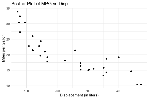
19.9.2.3 Box Plot: body_mass by island from penguins
Agent step: 1
Step passed evaluation and execution.Generated code:library(ggplot2)
ggplot(penguins, aes(x = island, y = body_mass)) +
geom_boxplot(notch = TRUE) +
labs(
title = "Box Plot of Body Mass by Island",
x = "Island",
y = "Body Mass"
) +
theme_minimal() 
19.9.3 What This Agent Can and Cannot Do
19.9.3.1 What It Can Do
The balanced agent demonstrates several capabilities that go well beyond the simple agent and the basic workflow examples earlier in this chapter:
- Natural language task specification: the user describes the goal in plain language — no R syntax, no function names. The agent translates that description into working, executable code.
- Flexible tool selection: the same
run_agent()interface handles summaries, scatter plots, and box plots. The agent selects the appropriate tool based on the task description without the user specifying which function to call. - Portable across datasets: every tool accepts dataset and variable names as parameters, so the same agent works with
mtcars,penguins, or any other data frame without modification. - Structured evaluation before execution: generated code is checked against explicit contracts before it is run, catching structural and constraint violations without consuming a runtime error.
- Iterative self-improvement: when a step fails, the agent refines its prompt using targeted feedback and tries again, converging on correct output across multiple attempts.
- Full execution history: every run produces a structured debug log that makes the agent’s reasoning transparent and diagnosable.
19.9.3.2 What It Cannot Do
The balanced agent handles one task per call. Each call to run_agent() selects one action, executes it, and returns.
- There is no mechanism for the agent to complete a summary and then use those results to inform a subsequent plot — the two calls are independent and share no state.
Consider a task like: “Create a scatter plot of the two numeric variables with the highest means in mtcars.” This requires two dependent steps:
- Summarize the data to identify the two variables with the highest means
- Use those variable names to generate the scatter plot
The current agent cannot do this because the result of step 1 is not available to step 2. Each run_agent() call starts fresh with no memory of prior calls.
- Handling tasks like this requires persistent memory — a mechanism for storing intermediate results and making them available to subsequent steps.
- This is the natural next extension of the system built here and points toward the more sophisticated agent architectures covered in later sections.
19.10 Adding a New Tool: A Deterministic Example
The balanced agent is designed to be extended. Adding a new tool requires changes in exactly four places:
- A new tool file in
R/tools/containing the function and any supporting code - A new registry entry in
make_tool_registry()mapping the action name to the function - A new source line in
source_config.Rto load the tool file - A new action in
choose_action()so the model knows the tool exists
Nothing else in the system changes — the agent loop, the helper functions, and the existing tools are untouched.
This is the extensibility benefit of the registry pattern in practice.
19.10.1 Deterministic vs Prompt-Based Tools
The three tools built so far, summary, scatter plot, and box plot, are all prompt-based: they ask the model to generate code, then extract, evaluate, and execute it.
- This pipeline is necessary when the output is genuinely variable and the model adds value by deciding how to construct the code.
Not every tool needs this pipeline. A deterministic tool wraps existing R code that always produces the same structure given the same input.
For these tools, code generation introduces unnecessary complexity:
- The model may generate syntactically different but semantically equivalent calls across runs
- Each variation requires evaluation logic to catch and retry logic to handle each failure mode
- A function that cannot fail meaningfully does not benefit from a generate/evaluate/retry cycle
For deterministic tools the right pattern is a direct call wrapper: a function that validates inputs, calls the underlying R function, wraps the result in the same success/value structure the agent loop expects, and returns.
- No model call, no code extraction, no evaluation, no retry.
This illustrates a general principle: use code generation where the output is genuinely variable and the model adds value; use direct calls where the output is predictable and deterministic.
- The tool registry accommodates both patterns as the dispatch logic checks which kind of result was returned and handles it accordingly.
19.10.2 Input Validation for Deterministic Tools
Input validation belongs in the wrapper, not in the underlying function.
This reflects a deliberate separation of concerns:
- The underlying function (
vars_df()below) is a general-purpose analytical tool designed to be called directly by users.- Its
stopifnot()checks throw informative errors for interactive use, which is the right behavior for a standalone function.
- Its
- The wrapper (
call_vars_df()) is an agent tool.- It must return a structured
success/valuelist regardless of outcome, because the agent loop expects that structure from every tool. - Throwing an error from inside the wrapper would bypass the debug log and produce an unhandled exception in the loop.
- It must return a structured
Validating inputs in the wrapper before calling the underlying function means failures are caught early, formatted as structured results, and surfaced cleanly through the debug log.
- Relying on
tryCatch()alone to catch errors thrown by the underlying function works but produces less informative messages that are harder to diagnose.
The general rule for deterministic tool wrappers:
- Validate inputs explicitly and return a structured failure if they do not meet requirements
- Call the underlying function inside
tryCatch()as a safety net for unexpected errors - Return a named list with
success,value, anderrorfields — the same structure assafe_execute_code().
The agent loop detects which pattern was used by checking whether the generate closure returned a list with a success field (matching the direct call pattern) or a raw character string (matching the prompt-based pattern).
- The two deterministic and prompt tool paths are handled differently in the dispatch block but both paths produce the same structured result the rest of the loop can consume and interpret.
NoteWhat Appears in the Debug Log for Deterministic Tools
When print_agent_debug() shows NULL for raw_code, code, and eval_result on a deterministic tool step this is expected since the tool was called directly rather than through code generation.
- The
exec_resultfield still shows the outcome and returned value. - The
tool_typefield identifies the step as deterministic so you can distinguish it from a prompt-based step that failed to generate code.
19.10.3 Example: Inspecting Data Frame Variables
To demonstrate adding a deterministic tool, we will build vars_df()— a function that inspects the variables in a data frame and returns a tibble with the name, type, class, number of unique values, and number of NAs for each variable.
Adding vars_df() as a tool extends what the agent can do meaningfully. With variable characteristics available as data, the agent can:
- identify numeric variables for a scatter plot
- identify categorical variables for a box plot grouping variable
- find the variables with the highest means
These intermediate results can be used by persistent memory to support other tools.
vars_df() is a natural candidate for a deterministic tool.
- The output structure is always the same tibble regardless of the input data; there is nothing for code generation to decide and nothing for evaluation to check.
The tool file contains two functions that work together as a pair, following the same pattern as the generate/evaluate pairs:
vars_df(): the underlying analytical function, general-purpose and independently useful, withstopifnot()checks appropriate for interactive usecall_vars_df(): the direct call wrapper, agent-specific, validates inputs before callingvars_df(), and always returns a structuredsuccess/valueresult
We introduce each in turn before showing the complete tool file and the four changes needed to register it with the agent.
19.10.3.1 vars_df() — The Analytical Function
vars_df() takes a data frame and returns a tibble with one row per variable describing five characteristics as in Table 19.5.
| Column | What it contains |
|---|---|
var_name |
Variable name |
type |
Storage type from typeof() — e.g., "double", "integer", "character" |
class |
Class from class() — e.g., "numeric", "factor", "POSIXct" |
var_unique |
Number of distinct non-NA values |
var_na |
Number of NA values |
The combination of type and class together is more informative than either alone
typedescribes how the value is stored in memory,classdescribes how R treats it analytically.- A factor, for example, has
type = "integer"butclass = "factor". - Both pieces of information are useful when deciding which variables are appropriate for a given plot or analysis.
var_unique is particularly useful for distinguishing continuous numeric variables from discrete ones
- a variable with two unique values is likely binary, one with five to ten is likely ordinal or categorical, and one with many unique values is likely continuous.
The function uses stopifnot() to validate that the input is a data frame with at least one row and one column.
- These checks are appropriate for a general-purpose function called interactively — they throw informative errors immediately when the input is wrong.
- The direct call wrapper
call_vars_df()handles these same cases differently:- rather than letting the errors propagate, it catches them and returns a structured failure that the agent loop can log and surface through the debug output.
- This is the separation of concerns between the analytical function and its agent wrapper in practice.
19.10.3.2 call_vars_df() — The Direct Call Wrapper
call_vars_df() is the agent-facing interface to vars_df().
- It accepts the data frame name as a string, retrieves the object from the calling environment, validates the inputs, calls
vars_df(), and returns a structured result.
The wrapper follows the three-step rule for deterministic tool wrappers established earlier:
Step 1 — Explicit input validation before calling the underlying function.
- The wrapper checks that
df_nameis a non-empty string, that an object with that name exists in the environment, and that the object is a data frame with at least one row and column. - Each check returns a structured failure with a specific message rather than letting the error propagate to
vars_df():- A missing or empty
df_namereturns: “df_name must be a non-empty string.” - A name that does not exist in the environment returns: “‘mtcars’ not found in the current environment.”
- An object that is not a data frame returns: “‘x’ is not a data frame.”
- A data frame with no rows or columns returns the corresponding message
- A missing or empty
These specific messages surface in the debug log and can inform prompt refinement so the agent knows exactly what went wrong rather than receiving a generic error.
Step 2 — tryCatch() as a safety net.
- After the explicit checks,
vars_df()is called insidetryCatch()to catch any unexpected errors that the validation did not anticipate. - This is defensive programming — the explicit checks handle the expected failure modes,
tryCatch()handles the rest.
Step 3 — Structured return.
- Every exit path returns a named list with
success,value, anderrorfields, the same structure assafe_execute_code(). - The agent loop detects this structure and routes to the deterministic dispatch path rather than the prompt-based path.
One additional argument worth noting: envir = parent.frame() defaults to looking for the data frame in the calling environment.
- In the agent loop this means the data frame must be available in the environment where
run_agent()was called. - This is the same requirement that applies to
safe_execute_code()for all prompt-based tools. - Users working interactively will find that any data frame loaded in their R session is automatically available.
With both functions described, Listing 19.42 shows the complete tool file:
Source for tool_vars_df.R (in tools )
# tool_vars_df.R
# Deterministic tool for inspecting data frame variable characteristics.
# Unlike prompt-based tools, vars_df() is called directly — no code
# generation, evaluation, or retry logic is needed.
#
#   vars_df()          — returns variable characteristics as a tibble
#   call_vars_df()     — wraps vars_df() for direct registration in
#                        the tool registry

# Variable characteristics ----

vars_df <- function(df) {
  stopifnot(
    "input is not a data frame" = is.data.frame(df),
    "input does not have at least 1 row" = nrow(df) >= 1,
    "input does not have at least 1 column" = ncol(df) >= 1
  )
  tibble::tibble(
    var_name = names(df),
    type = purrr::map_chr(df, typeof),
    class = purrr::map_chr(df, \(v) stringr::str_c(class(v), collapse = " ")),
    var_unique = purrr::map_int(df, \(col) {
      dplyr::n_distinct(col, na.rm = TRUE)
    }),
    var_na = purrr::map_int(df, \(col) sum(is.na(col)))
  )
}

# Direct call wrapper ----

call_vars_df <- function(df_name, envir = parent.frame()) {
  tryCatch(
    {
      df <- get(df_name, envir = envir)
      list(
        success = TRUE,
        value = vars_df(df)
      )
    },
    error = function(e) {
      list(
        success = FALSE,
        value = NULL,
        error = conditionMessage(e)
      )
    }
  )
}
roxygen2 documentation: vars_df() and call_vars_df()
# tool_vars_df.R
# Deterministic tool for inspecting data frame variable characteristics.
# Unlike prompt-based tools, vars_df() is called directly — no code
# generation, evaluation, or retry logic is needed.
#
#   vars_df()          — returns variable characteristics as a tibble
#   call_vars_df()     — wraps vars_df() for direct registration in
#                        the tool registry

# Variable characteristics ----

#' Show characteristics of data frame variables
#'
#' Creates a tibble with a row for each variable and columns for the
#' variable name, type, class, number of unique values, and number
#' of NA values. Used as a deterministic tool in the agent registry
#' to inspect a data frame before selecting variables for analysis.
#'
#' @param df A data frame with at least one row and at least one column.
#'
#' @return A tibble with \code{ncol(df)} rows and five columns:
#'   \describe{
#'     \item{\code{var_name}}{Character. Variable name.}
#'     \item{\code{type}}{Character. Storage type from \code{typeof()}.}
#'     \item{\code{class}}{Character. Class from \code{class()},
#'       collapsed if multiple.}
#'     \item{\code{var_unique}}{Integer. Number of distinct non-NA values.}
#'     \item{\code{var_na}}{Integer. Number of NA values.}
#'   }
#'
#' @seealso \code{\link{call_vars_df}}
vars_df <- function(df) {
  stopifnot(
    "input is not a data frame" = is.data.frame(df),
    "input does not have at least 1 row" = nrow(df) >= 1,
    "input does not have at least 1 column" = ncol(df) >= 1
  )
  tibble::tibble(
    var_name = names(df),
    type = purrr::map_chr(df, typeof),
    class = purrr::map_chr(df, \(v) stringr::str_c(class(v), collapse = " ")),
    var_unique = purrr::map_int(df, \(col) {
      dplyr::n_distinct(col, na.rm = TRUE)
    }),
    var_na = purrr::map_int(df, \(col) sum(is.na(col)))
  )
}


# Direct call wrapper ----

#' Call vars_df() by data frame name for use in the tool registry
#'
#' A thin wrapper around \code{vars_df()} that accepts a data frame
#' name as a string and retrieves the object from the calling
#' environment. Designed for direct registration in the tool registry
#' without going through code generation, extraction, or evaluation.
#'
#' Unlike prompt-based tools, this function is deterministic: the
#' output structure is always a tibble with the same five columns.
#' There is no need for a generate/evaluate pair, retry logic, or
#' \code{process_agent_step()} — the result is returned directly.
#'
#' @param df_name Character. Name of the data frame as a string
#'   (e.g., \code{"mtcars"}). The object must exist in the calling
#'   environment.
#' @param envir Environment. Where to look for \code{df_name}.
#'   Defaults to \code{parent.frame()}.
#'
#' @return A named list with two elements:
#'   \describe{
#'     \item{\code{success}}{Logical. TRUE if the data frame was
#'       found and \code{vars_df()} completed without error.}
#'     \item{\code{value}}{The tibble returned by \code{vars_df()},
#'       or NULL on failure.}
#'   }
#'
#' @seealso \code{\link{vars_df}}
call_vars_df <- function(df_name, envir = parent.frame()) {
  tryCatch(
    {
      df <- get(df_name, envir = envir)
      list(
        success = TRUE,
        value = vars_df(df)
      )
    },
    error = function(e) {
      list(
        success = FALSE,
        value = NULL,
        error = conditionMessage(e)
      )
    }
  )
}
ImportantConverting Existing Functions into Tools
The pattern used here applies broadly.Almost any deterministic R function you have already written can become a tool in an agent with two additions:
- a direct call wrapper that validates inputs and returns a structured result, and
- a registry entry that maps an action name to the wrapper. T
The underlying function does not need to change at all.
The one qualification is that the function should produce output the agent can use meaningfully — either a value it can return directly to the user, or a structured result another tool or the persistent memory system can consume in a subsequent step.
vars_df()satisfies both: its tibble output is useful on its own and directly actionable as input to the variable selection logic in the memory example that follows.
Functions that have side effects — writing files, modifying global state, sending network requests — can also be wrapped as tools, but they require more careful consideration of what happens when the agent retries or the loop runs more steps than expected.
Deterministic functions with no side effects are the simplest and safest starting point.
19.10.4 Updating the Agent to Include the New Tool
We have created a new tool. Now we need to add it to the available tools for this agent.
Three small changes register vars_df() with the balanced agent.
- Each change is in a different file, and none of them touch the agent loop or any existing tool.
Note
The steps below are notional since the files shown throughout this chapter already include these changes since vars_df() is part of the complete agent.
- They are presented here to make explicit what you would do when extending the agent with a new tool during iterative development.
- In practice, adding a new tool to the balanced agent is exactly this: three small, targeted changes in three specific places, with nothing else in the system requiring modification.
The steps are the same regardless of whether the new tool is deterministic or prompt-based, only the content of the tool file and registry entry differs.
19.10.4.1 Step 1: Source the tool file — source_config.R
Add one line to load tool_vars_df.R. You could put it before existing tools to follow an analytical flow or after to show it is a new capability as the order does not matter to the system.
19.10.4.2 Step 2: Add the registry entry — make_tool_registry()
Add one entry to the registry in agent_balanced.R. Placing it at the end before Stop helps preserve the development history:
# --- Inspect variable characteristics (deterministic) ---
# call_vars_df() is invoked directly — no code generation,
# evaluation, or retry logic needed. The success field in
# the return value signals to the dispatch block that this
# is a deterministic tool.
vars = list(
  label    = "variable characteristics",
  pattern = "^vars|^variable|^inspect|^describe|^attributes|
      ^characteristics|^schema|^structure|^columns|^fields",
  generate = function() call_vars_df(data_name, envir = envir),
  evaluate = function(result) list(
    success = result$success,
    checks  = list()
  )
),
19.10.4.3 Step 3: Add the action — choose_action()
Add vars to the available actions list in the prompt.
- The exact order is not important to the system, but the action must be mentioned in the prompt for the model to know it exists.
- However, placing it first might signal to the model that data inspection is a natural first step before analysis which could also make it more salient to the model and likely to be called instead of a plot.
- Let’s move it later in the code, before
stop:, to reduce the chances of it being called when no longer needed.
"Available actions:",
"- summarize: Compute the mean and standard deviation of the
        numeric columns of a data frame. Use this when
        you need numeric summaries of the data values.",
"- scatter: Create a scatter plot for two numeric variables.",
"- box: Create a box plot for a numeric variable grouped by a categorical variable.",
"- vars: Inspect the names, types, classes, and missing value
   counts for all variables in a data frame. Use this
   when you need to know what variables exist and their
   data types, not their numeric values.",
"- stop: Indicate that the task is complete.",
19.10.4.4 The Dispatch Block— run_agent()
The dispatch block in run_agent() was already shown in the complete function listing above, but its deterministic tool path was not explained at that point since vars_df() had not yet been introduced.
The dispatch block handles two paths based on what the matched tool’s generate closure returns:
- A raw character string signals a prompt-based tool — the string is the model’s response and needs to go through extraction, evaluation, and execution via
process_agent_step() - A list with a
successfield signals a deterministic tool — the result is already structured and ready to use, bypassing extraction, evaluation, and execution entirely
The check that distinguishes the two paths is:
This is the only place in the agent that needs to know whether a tool is deterministic or prompt-based.
- Every other part of the system, the registry, the debug log, the return value, treats both tool types identically.
- Adding another deterministic tool in the future requires no changes here.
With these changes in place, re-source the config, and the agent is ready to use the new tool:
The next section runs the agent on a vars task to confirm the tool works, then uses the result to motivate the persistent memory example.
19.10.5 Running the vars_df Tool
With the tool registered and the config updated, we can run the agent on a variable inspection task.
- The
penguinsdataset is a good choice here since it contains a mix of numeric, integer, factor, and character variables which givesvars_df()something meaningful to show.
Agent step: 1
Step passed evaluation and execution.# A tibble: 8 × 5
var_name type class var_unique var_na
<chr> <chr> <chr> <int> <int>
1 species integer factor 3 0
2 island integer factor 3 0
3 bill_len double numeric 164 2
4 bill_dep double numeric 80 2
5 flipper_len integer integer 55 2
6 body_mass integer integer 94 2
7 sex integer factor 2 11
8 year integer integer 3 0The result is a tibble with one row per variable. Notice:
species,island, andsexhaveclass = "factor", making them candidates for the categorical variable in a box plotbill_length,bill_depth,flipper_length, andbody_masshaveclass = "numeric"— candidates for scatter plot variables or a box plot numeric variableyearhasclass = "integer"— useful to know since it might look numeric but behaves differently in some contextsvar_naidentifies which variables have missing values.bill_length,bill_depth,flipper_length,body_mass, andsexall have NAs, which is why the box plot examples usedwarning: false
The debug log confirms the tool was called directly rather than through code generation:
====================
Step:   1
Action: vars
Status: success
====================
Step:   1
Action: vars
Status: success

Task before:
 Show the variable names, types, and
                      classes for all variables in the
                      penguins data frame.

Execution success: TRUE

Task after:
 Show the variable names, types, and
                      classes for all variables in the
                      penguins data frame.
At detail level, raw_code, code, and eval_result are all NULL which is the expected output for a deterministic tool step as noted earlier.
- The
exec_resultfield shows the tibble returned bycall_vars_df().
This result is now available as result_vars$value.
- This is a structured tibble that can be used programmatically to select variables for the next step.
- That is exactly what the persistent memory example does next: it uses
result_varsto identify the numeric variables with the highest means and passes them to a scatter plot call.
TipPractical Tips for Routing Actions with Small Local Models
Refining the vars action demonstrated three practical tips about working with small local models:
- Make action descriptions specific enough to distinguish between similar actions.
- The model confused
varsandsummarizeuntil their descriptions explicitly separated them. — One inspects variable structure, the other computes numeric values. - Clear distinctions in the
choose_action()prompt are often more effective than relying on the task description alone.
- The model confused
- Make patterns need to be broad enough to catch natural variations in how the model phrases its action choice.
- Small models do not always return the exact word you expect.
- Expanding the
varspattern inmake_tool_registry()to catch phrasings like “attributes”, “characteristics”, “schema”, and “structure” accommodates the range of reasonable responses without requiring the model to use a specific word.
- Use the debug log to diagnose routing failures.
- The
$actionvalue in the debug log shows exactly what the model returned. - If the model is consistently returning a valid response that fails to match the pattern, that is a signal to broaden the pattern.
- If it is returning the wrong action entirely, that is a signal to sharpen the action description.
- The debug log tells you which problem you have.
- The
Together the iterative adjustments illustrated the flexibility vs specificity tradeoff in practice:
- The action description needed to be more specific to route correctly, while the matching pattern needed to be more flexible to catch valid responses.
- Getting this balance right for a given model and task scope is part of the iterative refinement process that makes agentic systems work reliably.
19.11 Extending the Agent with Persistent Memory
The vars_df() tool makes variable characteristics available as data, but the balanced agent handles one task per call so the result of inspecting the variables cannot be passed directly to a subsequent plot call within the same agent run.
Consider this task: “Create a scatter plot of the two numeric variables with the highest means in the penguins data frame.” This requires two dependent steps:
- Inspect the variables to identify which are numeric
- Summarize the numeric variables to find the two with the highest means
- Use those variable names to generate the scatter plot
The current agent cannot do this in a single call because the result of step 1 is not available to step 2, and the result of step 2 is not available to step 3.
- Each
run_agent()call starts fresh with no memory of prior calls.
Let’s create a new agent called run_agent_memory() with a simple persistent memory mechanism that allows results to be passed between steps.
run_agent_memory()extends the balanced agent with amemoryargument, a named list of context from prior steps that is injected into the task description before action selection.- This is what memory means in a stateless system: the model has no persistent state between calls, so memory is simply context that gets injected into the next prompt (similar to many interactive chat systems).
- Using
run_agent_memory()to wraprun_agent()makes that mechanism explicit.
19.11.1 Running the Two-Step Task
The three-step task above becomes a coordinated sequence of agent calls, with each result informing the next: as seen in Listing 19.45, Listing 19.46, and Listing 19.47.
result_scatter <- run_agent_memory(
  task_description = "Create a scatter plot of the two
                      numeric variables with the most
                      unique values in the penguins
                      data frame.",
  data_name        = "penguins",
  x_var            = top_vars[1],
  y_var            = top_vars[2],
  memory           = list(
    "numeric variables with most unique values" =
      paste(top_vars, collapse = " and ")
  )
)

result_scatter$plot
The key difference from a standard run_agent() call is the memory argument.
- It carries the variable names identified in step 2 into the task description for step 3, so
choose_action()and the generate function both see the context from prior steps.
The memory is intentionally simple, a named list of plain-language summaries rather than a structured store.
- This is sufficient for passing results between a small number of sequential steps.
- The variable names are passed explicitly as
x_varandy_varparameters as well, which means the evaluate function can still check for the correct variables. - Memory provides context for the model’s decisions; the explicit parameters enforce the contract.
19.11.2 The Memory Configuration
run_agent_memory() is sourced via its own config file that builds on the balanced agent config
- The config file in Listing 19.48 sources everything the balanced agent needs and then adds the memory wrapper.
- This keeps the extension self-contained: to use the memory-extended agent, source one file.
Source for source_config_memory.R (in agent_config )
# source_config_memory.R
# Extends the balanced agent with memory injection.
# Sources the complete balanced agent configuration first,
# then adds run_agent_memory().
#
# Usage:
#   source(here::here("R/agent_config/source_config_memory.R"))

source(here::here("R/agent_config/source_config.R"))
source(here::here("R/agents/agent_balanced_memory.R"))
The two-line structure of source_config_memory.R is itself a nice point: extending the agent with a new capability means adding to the config, not rewriting it.
- The complete balanced agent, all four tools, all helper functions, all core functions, is loaded by the first line.
- The second line adds the one new function that provides memory injection.
19.11.3 What the Memory Wrapper Does
run_agent_memory() is a thin wrapper around run_agent() as shown in Listing 19.49.
- It does one thing: formats the memory entries as plain-language context and prepends them to the task description before passing everything to
run_agent(). - The agent loop, tool dispatch, evaluation, and debug logging are all handled by
run_agent()unchanged.
Source for agent_balanced_memory.R (in agents )
# agent_balanced_memory.R
# Memory-extended agent ----

run_agent_memory <- function(
  task_description,
  data_name,
  x_var = NULL,
  y_var = NULL,
  num_var = NULL,
  cat_var = NULL,
  smoother_method = NULL,
  model = "qwen2.5-coder:3b",
  max_steps = 5,
  envir = parent.frame(),
  verbose = TRUE,
  memory = NULL
) {
  # Inject memory into task description if provided.
  # Memory entries are formatted as plain-language context
  # appended after the original task so the model sees both
  # the goal and the relevant prior results.
  if (!is.null(memory) && length(memory) > 0) {
    memory_text <- paste(
      "Context from prior steps:",
      paste(
        names(memory),
        unlist(memory),
        sep = ": ",
        collapse = "\n"
      )
    )
    task_description <- paste(
      task_description,
      memory_text,
      sep = "\n\n"
    )
  }

  # Delegate to run_agent() with the updated task description.
  # All loop logic, tool dispatch, evaluation, and debug logging
  # are handled there — this function only adds memory injection.
  run_agent(
    task_description = task_description,
    data_name = data_name,
    x_var = x_var,
    y_var = y_var,
    num_var = num_var,
    cat_var = cat_var,
    smoother_method = smoother_method,
    model = model,
    max_steps = max_steps,
    envir = envir,
    verbose = verbose
  )
}
roxygen2 documentation: run_agent_memory()
# agent_balanced_memory.R
# Memory-extended agent ----

#' Run a goal-directed data analysis agent with memory
#'
#' Extends \code{run_agent()} with a \code{memory} argument that
#' accepts a named list of context from prior steps. When provided,
#' memory entries are formatted as plain-language context and
#' prepended to the task description before action selection,
#' allowing the agent to use results from previous calls when
#' generating code or selecting variables.
#'
#' All other behaviour is identical to \code{run_agent()}. The
#' agent loop, tool dispatch, evaluation, and debug logging are
#' unchanged. Memory is simply additional context that the model
#' sees as part of the task description.
#'
#' This wrapper illustrates a general principle: adding a new
#' capability to the agent does not require modifying the agent
#' loop. Memory injection is a pre-processing step that delegates
#' to \code{run_agent()} for everything else. Any improvement to
#' \code{run_agent()} is automatically inherited here.
#'
#' @param task_description Character. Natural language description
#'   of the analysis task.
#' @param data_name Character. Name of the data frame as a string
#'   (e.g., \code{"mtcars"}).
#' @param x_var Character or NULL. x-axis variable for scatter
#'   plots.
#' @param y_var Character or NULL. y-axis variable for scatter
#'   plots.
#' @param num_var Character or NULL. Numeric variable for box
#'   plots.
#' @param cat_var Character or NULL. Categorical variable for box
#'   plots.
#' @param smoother_method Character or NULL. Smoother method for
#'   scatter plots (e.g., \code{"lm"}). NULL means no smoother.
#' @param model Character. Ollama model to use across all calls.
#'   Defaults to \code{"qwen2.5-coder:3b"}.
#' @param max_steps Integer. Maximum number of agent steps.
#'   Defaults to 5.
#' @param envir Environment. Passed to \code{run_agent()} for
#'   code execution and data frame lookup. Defaults to
#'   \code{parent.frame()}.
#' @param verbose Logical. If TRUE prints step progress.
#'   Defaults to TRUE.
#' @param memory Named list or NULL. Context from prior agent
#'   steps to inject into the task description. Each element
#'   should be a plain-language summary of a prior result, named
#'   to describe what it represents (e.g.,
#'   \code{list("variables with highest means" = "hp and disp")}).
#'   NULL means no memory is injected (default).
#'
#' @return Invisibly returns the same named list as
#'   \code{run_agent()}: success, action, code, eval_result,
#'   parse_result, exec_result, value, plot, and debug_log.
#'
#' @seealso \code{\link{run_agent}}, \code{\link{choose_action}},
#'   \code{\link{make_tool_registry}},
#'   \code{\link{print_agent_debug}}
run_agent_memory <- function(
  task_description,
  data_name,
  x_var = NULL,
  y_var = NULL,
  num_var = NULL,
  cat_var = NULL,
  smoother_method = NULL,
  model = "qwen2.5-coder:3b",
  max_steps = 5,
  envir = parent.frame(),
  verbose = TRUE,
  memory = NULL
) {
  # Inject memory into task description if provided.
  # Memory entries are formatted as plain-language context
  # appended after the original task so the model sees both
  # the goal and the relevant prior results.
  if (!is.null(memory) && length(memory) > 0) {
    memory_text <- paste(
      "Context from prior steps:",
      paste(
        names(memory),
        unlist(memory),
        sep = ": ",
        collapse = "\n"
      )
    )
    task_description <- paste(
      task_description,
      memory_text,
      sep = "\n\n"
    )
  }

  # Delegate to run_agent() with the updated task description.
  # All loop logic, tool dispatch, evaluation, and debug logging
  # are handled there — this function only adds memory injection.
  run_agent(
    task_description = task_description,
    data_name = data_name,
    x_var = x_var,
    y_var = y_var,
    num_var = num_var,
    cat_var = cat_var,
    smoother_method = smoother_method,
    model = model,
    max_steps = max_steps,
    envir = envir,
    verbose = verbose
  )
}
This wrapper pattern is worth noting:
run_agent_memory()adds one capability, memory injection, without duplicating any of the agent logic.- Any improvement to
run_agent()is automatically inherited. - This is the same separation of concerns applied throughout the system: each function does one thing, and composition handles the rest.
The persistent memory approach used here, carrying results forward explicitly as context, is the simplest form of agent memory.
- More sophisticated systems use external storage and retrieval to manage memory across longer task horizons and multiple agents.
- That is one of the defining challenges in agentic system design and points toward the more advanced architectures introduced in the next section.
19.11.4 Running the Memory-Extended Agent
With source_config_memory.R sourced, the three-step task is now executable and we can run each in turn.
The first step is to run the standard run_agent() to inspect the penguins variables.
- The result is a tibble in the global environment we can use in R to identify the two numeric variables with the most unique values.
- The third step passes those variable names both as explicit parameters and as memory context to
run_agent_memory().
Agent step: 1
Step passed evaluation and execution.# A tibble: 8 × 5
var_name type class var_unique var_na
<chr> <chr> <chr> <int> <int>
1 species integer factor 3 0
2 island integer factor 3 0
3 bill_len double numeric 164 2
4 bill_dep double numeric 80 2
5 flipper_len integer integer 55 2
6 body_mass integer integer 94 2
7 sex integer factor 2 11
8 year integer integer 3 0- The tibble shows which variables are numeric, integer, factor, and character.
The second step is to run top_vars() which uses this variable from the first step to create an internal data frame to identify the two numeric variables with the most unique values.
- Note: no model call is needed, just standard dplyr:
[1] "bill_len" "bill_dep"The third step is to run run_agent_memory().
- This uses the data frame values
- as explicit parameters, so the evaluate function can check for the correct variables, and,
- as memory context, so the model understands why those variables were chosen:
result_scatter <- run_agent_memory(
  task_description = "Create a scatter plot of the two
                      numeric variables with the most
                      unique values in the penguins
                      data frame.",
  data_name        = "penguins",
  x_var            = top_vars[1],
  y_var            = top_vars[2],
  memory           = list(
    "numeric variables with most unique values" =
      paste(top_vars, collapse = " and ")
  )
)
Agent step: 1
Step failed. Refining prompt...
Agent step: 2
Step failed. Refining prompt...
Agent step: 3
Step failed. Refining prompt...
Agent step: 4
Step failed. Refining prompt...
Agent step: 5
Step failed. Refining prompt...
Maximum steps reached without completing the task.NULLThe three steps illustrate how the pieces fit together.
vars_df()provides structured data about the data frame that R code can manipulate directly.- The memory argument carries the result of that manipulation into the next agent call as plain-language context.
- The explicit variable name parameters ensure the evaluate function can still enforce the contract regardless of what the model decides to do with the memory context.
This is the simplest form of persistent memory, using the global environment for carrying results forward explicitly between calls.
- The model remains stateless; the caller manages the state.
- For the class of tasks where intermediate results can be extracted and summarized as plain text, this pattern is sufficient and requires no additional infrastructure.
19.12 Extending to A Single-Call Pipeline
The three-step sequence works but requires the caller to manage the intermediate result, extracting top_vars from result_vars$value and passing it to run_agent_memory().
For a task where the intermediate result is purely instrumental, this can be wrapped in a pipeline function that handles the orchestration internally and exposes a single call to the user.
run_agent_pipeline() encapsulates the three steps:
- it inspects the variables,
- extracts the top two numeric variables in R, and
- passes them to
run_agent_memory()for the scatter plot.
The caller provides only the plot task description and the data frame name.
source_config_pipeline.R follows the same two-line pattern established for the memory config as seen in Listing 19.55.
- It sources the memory config first, inheriting everything the balanced agent needs plus
run_agent_memory(), then addsrun_agent_pipeline():
Source for source_config_pipeline.R (in agent_config )
# source_config_pipeline.R
# Extends the memory agent with pipeline orchestration.
# Sources the memory agent configuration first, then adds
# run_agent_pipeline().
#
# Usage:
#   source(here::here("R/agent_config/source_config_pipeline.R"))

source(here::here("R/agent_config/source_config_memory.R"))
source(here::here("R/agents/run_agent_pipeline.R"))
Each config file in the system builds on the one below it:
source_config.Rloads the complete balanced agentsource_config_memory.Raddsrun_agent_memory()source_config_pipeline.Raddsrun_agent_pipeline()
Sourcing source_config_pipeline.R gives you all three agents (run_agent(), run_agent_memory(), and run_agent_pipeline()) loaded and ready to use as seen in Listing 19.56.
Source for run_agent_pipeline.R (in agents )
# agent_pipeline.R
# Pipeline orchestration ----

run_agent_pipeline <- function(
  task_description,
  data_name,
  model = "qwen2.5-coder:3b",
  max_steps = 5,
  verbose = TRUE
) {
  # Step 1: inspect variable characteristics
  # Uses the vars tool to get a structured tibble describing
  # each variable in the data frame
  result_vars <- run_agent(
    task_description = paste(
      "Show the variable names, types, and classes for all",
      "variables in the",
      data_name,
      "data frame."
    ),
    data_name = data_name,
    model = model,
    max_steps = max_steps,
    verbose = verbose
  )

  # Guard: return early if step 1 failed to produce a result
  if (!result_vars$success || is.null(result_vars$value)) {
    message("Pipeline failed at step 1: could not inspect variables.")
    return(invisible(NULL))
  }

  # Step 2: extract the two numeric variables with the most
  # unique values — handled in R, no model call needed
  top_vars <- result_vars$value |>
    dplyr::filter(class == "numeric") |>
    dplyr::arrange(dplyr::desc(var_unique)) |>
    dplyr::slice_head(n = 2) |>
    dplyr::pull(var_name)

  # Guard: return early if fewer than two numeric variables found
  if (length(top_vars) < 2) {
    message(
      "Pipeline failed at step 2: fewer than two numeric variables ",
      "found in ",
      data_name,
      "."
    )
    return(invisible(NULL))
  }

  if (verbose) {
    cat(
      "Step 2: top two numeric variables identified as",
      paste(top_vars, collapse = " and "),
      "\n"
    )
  }

  # Step 3: scatter plot using variable names from step 2
  # Memory carries the variable names as context so the model
  # understands why those variables were chosen
  run_agent_memory(
    task_description = task_description,
    data_name = data_name,
    x_var = top_vars[1],
    y_var = top_vars[2],
    memory = list(
      "numeric variables with most unique values" = paste(
        top_vars,
        collapse = " and "
      )
    ),
    model = model,
    max_steps = max_steps,
    verbose = verbose
  )
}
roxygen2 documentation: run_agent_pipeline()
# agent_pipeline.R
# Pipeline orchestration ----

#' Run a three-step pipeline: inspect variables, find variables,
#' then scatter plot
#'
#' Orchestrates two agent calls to complete a task that requires
#' intermediate results. First calls \code{run_agent()} to inspect
#' variable characteristics using \code{vars_df()}, then extracts
#' the two numeric variables with the most unique values and passes
#' them to \code{run_agent_memory()} to generate a scatter plot.
#'
#' This pipeline demonstrates how multi-step tasks can be
#' encapsulated in a single function call once the individual
#' steps are reliable. The intermediate result — the two variable
#' names — is managed internally as a local variable rather than
#' requiring the caller to handle it in the global environment.
#'
#' @param task_description Character. Natural language description
#'   of the scatter plot task passed to \code{run_agent_memory()}.
#'   Should describe the plot goal without specifying variable
#'   names — those are determined automatically from step 1.
#' @param data_name Character. Name of the data frame as a string
#'   (e.g., \code{"penguins"}). Used in both agent calls.
#' @param model Character. Ollama model to use across all calls.
#'   Defaults to \code{"qwen2.5-coder:3b"}.
#' @param max_steps Integer. Maximum number of steps passed to
#'   each agent call. Defaults to 5.
#' @param verbose Logical. If TRUE prints step progress for both
#'   agent calls. Defaults to TRUE.
#'
#' @return Invisibly returns the result of \code{run_agent_memory()}
#'   from step 3 — a named list with success, action, code,
#'   eval_result, parse_result, exec_result, value, plot, and
#'   debug_log. Returns NULL with a message if step 1 fails to
#'   produce variable characteristics.
#'
#' @seealso \code{\link{run_agent}}, \code{\link{run_agent_memory}},
#'   \code{\link{vars_df}}, \code{\link{call_vars_df}}
run_agent_pipeline <- function(
  task_description,
  data_name,
  model = "qwen2.5-coder:3b",
  max_steps = 5,
  verbose = TRUE
) {
  # Step 1: inspect variable characteristics
  # Uses the vars tool to get a structured tibble describing
  # each variable in the data frame
  result_vars <- run_agent(
    task_description = paste(
      "Show the variable names, types, and classes for all",
      "variables in the",
      data_name,
      "data frame."
    ),
    data_name = data_name,
    model = model,
    max_steps = max_steps,
    verbose = verbose
  )

  # Guard: return early if step 1 failed to produce a result
  if (!result_vars$success || is.null(result_vars$value)) {
    message("Pipeline failed at step 1: could not inspect variables.")
    return(invisible(NULL))
  }

  # Step 2: extract the two numeric variables with the most
  # unique values — handled in R, no model call needed
  top_vars <- result_vars$value |>
    dplyr::filter(class == "numeric") |>
    dplyr::arrange(dplyr::desc(var_unique)) |>
    dplyr::slice_head(n = 2) |>
    dplyr::pull(var_name)

  # Guard: return early if fewer than two numeric variables found
  if (length(top_vars) < 2) {
    message(
      "Pipeline failed at step 2: fewer than two numeric variables ",
      "found in ",
      data_name,
      "."
    )
    return(invisible(NULL))
  }

  if (verbose) {
    cat(
      "Step 2: top two numeric variables identified as",
      paste(top_vars, collapse = " and "),
      "\n"
    )
  }

  # Step 3: scatter plot using variable names from step 2
  # Memory carries the variable names as context so the model
  # understands why those variables were chosen
  run_agent_memory(
    task_description = task_description,
    data_name = data_name,
    x_var = top_vars[1],
    y_var = top_vars[2],
    memory = list(
      "numeric variables with most unique values" = paste(
        top_vars,
        collapse = " and "
      )
    ),
    model = model,
    max_steps = max_steps,
    verbose = verbose
  )
}
The pipeline reduces the three-step manual sequence to a single call:
Agent step: 1
Step passed evaluation and execution.
Step 2: top two numeric variables identified as bill_len and bill_dep
Agent step: 1
Step passed evaluation and execution.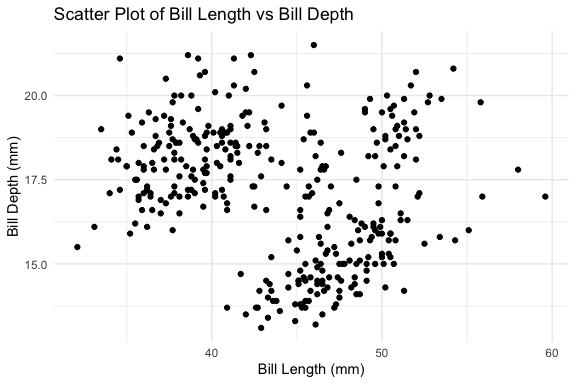
The pipeline illustrates a natural progression in system design: once individual steps are reliable, encapsulating them as a function makes the pattern reusable and hides orchestration details from the caller.
- The same principle that motivated wrapping individual prompts as functions now applies at the workflow level.
Whether to expose the steps explicitly or wrap them in a pipeline depends on whether intermediate results are useful to the caller.
- In exploratory analysis, seeing
result_varsafter step 1 may be informative. - In a production workflow, a single pipeline call is cleaner.
- Both are valid — the system supports either approach without modification.
Important
It is worth being precise about what “persistent memory” means in this implementation.
- The memory is not stored inside the agent —
run_agent()andrun_agent_memory()are both stateless functions that start fresh on every call. - The persistence comes from R’s global environment.
result_varsassigned in step 1 persists in the global environment and is available to steps 2 and 3.- The
memoryargument in step 3 takes that global object, formats it as plain text, and injects it into the prompt — but the agent itself never sees the R object, only the text representation of it.
This means the pattern works in any context where the global environment persists between calls:
- In a Quarto document: across chunk evaluations in the same render session
- In an interactive R session: across sequential calls at the console
- In a script: across sequential lines of top-level code
It does not work across separate R sessions, separate render runs, or separate script executions — each starts with a fresh global environment.
- For memory that persists across sessions, external storage such as a file, database, or vector store would be needed.
The run_agent_pipeline() function wraps the three steps into a single call precisely because the intermediate result — top_vars — does not need to be visible in the global environment.
- The pipeline manages it internally as a local variable, which is cleaner when the intermediate result is purely instrumental.
19.13 Balanced Agent Summary
At this point in the chapter we have built a complete agentic data analysis system from scratch, progressing through four levels of increasing capability:
- Interactive prompting established the foundation — writing effective prompts and understanding how models respond
- Structured prompts as functions converted one-time interactions into repeatable, testable, versionable code
- Workflows organized functions into fixed sequences with evaluation and retry logic
- Agents shifted control from fixed sequences to model-driven decision making, with tools the model can choose to invoke
The balanced agent that emerged from this progression consists of 16 functions across five directories, organized into four layers: core model interface, shared infrastructure, task-specific tools, and agent orchestration.
Three agents of increasing capability were built on this foundation:
run_agent()— single-task, model-driven action selection with structured evaluation and iterative refinementrun_agent_memory()— extends the balanced agent with context injection between calls from the global environmentrun_agent_pipeline()— orchestrates multiple agent calls into a single user-facing function
The final directory structure looked like
R/
├── agent_config/
│   ├── source_config.R              # balanced agent
│   ├── source_config_memory.R       # memory-extended agent
│   └── source_config_pipeline.R     # pipeline agent
├── agent_helpers/
│   ├── agent_debug.R                # print_agent_debug()
│   ├── agent_execution.R            # extract_code()
│   │                                # safe_execute_code()
│   ├── agent_feedback.R             # build_eval_feedback()
│   └── agent_step.R                 # process_agent_step()
├── agents/
│   ├── agent_balanced.R             # make_tool_registry()
│   │                                # choose_action()
│   │                                # run_agent()
│   ├── agent_balanced_memory.R      # run_agent_memory()
│   └── agent_pipeline.R             # run_agent_pipeline()
├── core/
│   ├── core_model.R                 # get_model_response()
│   └── core_ollama.R                # call_ollama()
└── tools/
    ├── tool_boxplot.R               # generate_code_boxplot()
    │                                # evaluate_code_boxplot()
    ├── tool_scatterplot.R           # generate_code_scatterplot()
    │                                # evaluate_code_scatterplot()
    ├── tool_summary_numeric.R       # generate_code_summary_numeric()
    │                                # evaluate_code_summary_numeric()
    └── tool_vars_df.R               # vars_df()
                                     # call_vars_df()
Each extension added one new file and two lines to a config — nothing else in the system changed.
- That extensibility is a direct consequence of the design patterns applied throughout: separation of concerns, layered architecture, design by contract, informative failure, documentation as specification, and configuration as composition.
The next section moves from building agents to working with agentic systems and shows how the concepts and patterns developed here appear at larger scale and how requirements and choices can affect working effectively within those systems.
NoteWhat The Balanced Agent Code Demonstrates Beyond the Agent Itself
The balanced agent is one of the more complex systems in these notes, not because any individual function is particularly difficult, but because of how many functions work together across multiple files to produce a coherent, extensible system. That integration is itself worth reflecting on.
The code demonstrates several best practices in modern data science development that apply well beyond agentic systems:
Separation of concerns.
- Each function does one thing.
extract_code()extracts,safe_execute_code()executes,build_eval_feedback()builds feedback,process_agent_step()orchestrates.
- No function reaches into another function’s responsibilities, making each independently testable and replaceable without touching the rest of the system.
Layered architecture.
- The system is organized into layers, core, helpers, tools, and agent, where each layer depends only on the layers below it.
- Adding a new tool does not require touching the core or helper layers.
- Extending the agent with memory or a pipeline required adding one new file and two lines to a config.
- This is the same principle behind well-designed R packages, database schemas, and software systems generally.
Design by contract.
- Every generate/evaluate pair defines an explicit contract: what the code should do, how it should be written, and what it must avoid.
- The evaluate function makes that contract testable.
- This pattern — specify, implement, verify — is the foundation of reliable data pipelines and reproducible analysis workflows.
Failing informatively.
- Every failure in the system produces structured output rather than stopping execution. Errors become data.
process_agent_step()returns a structured result at every stage;safe_execute_code()captures runtime errors;call_vars_df()validates inputs and returns structured failures.
- Systems that handle failure gracefully are easier to debug, extend, and trust — the same principle behind
tryCatch()in R andtry/exceptin Python.
Documentation as specification.
- The roxygen2 comments are not just documentation — they are a formal statement of what each function promises to do and what it requires.
- The
@paramtags describe input contracts, - the
@returntags describe output contracts, and - the
@seealsotags make the dependency structure navigable.
- The
- Writing documentation alongside code rather than after tends to produce better-designed functions.
Configuration as composition.
- Three config files,
source_config.R,source_config_memory.R, andsource_config_pipeline.R, each define a different agent by specifying what they load. - Changing an agent’s capabilities means changing its configuration, not rewriting its logic.
- This is the same idea behind dependency injection, package management, and environment configuration in production systems.
Replacing branches with data structures.
- The tool registry replaced an
if/else ifblock with a named list. - Adding a new tool required one new registry entry as the loop never changed.
- This pattern — replacing conditional logic with a dispatch table — appears in plugin architectures, command routers, and event handlers across every programming language.
These practices are not unique to agentic systems; they appear in well-designed R packages, production data pipelines, and software engineering more broadly.
- The agent provided a concrete context for applying them together.
As you build your own systems, consider these patterns and tailor them in different forms and at different scales to meet your needs.
19.14 Working with Agents Beyond Local Models
In Section 19.8 we built a working agent from scratch using Ollama and a local model.
- That experience was intentional: writing the tool registry, the generate/evaluate loop, and the memory pattern yourself makes visible what every agent system — no matter how polished — is doing underneath.
You now have a mental model that transfers and this section extends that foundation into more general settings.
Most professional data science work happens in environments where local models are not the primary option:
- Cloud APIs offer more capable models,
- Institutional infrastructure provides managed access, and
- Purpose-built agent systems handle entire classes of tasks without requiring you to write scaffolding at all.
Understanding the landscape of options, and the reasoning behind choosing one over another, is as important as knowing how to use any specific system.
ImportantThe LLM landscape is genuinely unsettled.
LLMs and agentic systems are evolving rapidly, leapfrogging each other in capability, cost, and design.
- A system that leads today may be overtaken next quarter.
This is precisely why the focus here is on general frameworks for thinking about each approach rather than definitive rankings.
There are core questions one can ask about any system at a point in time:
- how does it handle tools, memory, and context?
- what does it cost and who owns the data?
- how repeatable and auditable are its outputs?
These questions remain stable even as the specific answers change.
While the ecosystem is large and rapidly evolving, the options for working with agents in practice fall into three broad categories:
Build your own with a cloud API: you write the agent logic yourself, as in Section 19.8, but call a cloud-hosted model instead of a local one. Maximum control, Maximum responsibility.
Agent Software Development Kits and frameworks: pre-built scaffolding handles the orchestration; you compose tools, define workflows, and configure behavior within an established structure. Less code, more convention.
Opinionated agent systems: a fully realized agent that you direct and configure rather than construct. The system makes most architectural decisions; your job is to scope tasks well, evaluate outputs, and integrate results.
No approach is universally best; each has strengths that align with particular problem types, constraints, and working contexts.
The sections below describe each approach in more detail followed by a decision framework (a comparison table and flow diagram) to help you map your problem to a particular approach.
19.14.1 The Landscape: Three Approaches
Before going into detail it helps to see the three approaches as points on two related dimensions.
The first dimension is how much scaffolding you provide.
- At one end you write everything: the loop, the tool registry, the context management, the stopping condition.
- At the other end, a production system provides all of that; you configure it with plain text and direct it with task descriptions.
- SDKs and frameworks sit in the middle.
The second dimension is how general-purpose the system is.
- Raw API access and SDKs are general: you can build an agent for any domain.
- Opinionated systems are typically purpose-built
- Claude Code is designed for software engineering tasks;
- other systems are optimized for customer support, document processing, or data pipelines.
General-purpose systems offer more flexibility; purpose-built systems offer better performance on their target tasks out of the box.
These two dimensions interact with three practical considerations that should drive most real-world choices:
- Cost and access.
- Cloud APIs charge per token.
- Costs are modest for exploratory work but accumulate quickly in agentic loops, where a single task may generate dozens of model calls.
- Most large organizations have negotiated enterprise access to one or more providers, making cost a secondary concern for practitioners inside those organizations.
- For independent researchers, students, and small teams, free tiers and lower-cost providers matter more.
- Several providers e.g., Groq and Google AI Studio, offer free tiers sufficient for learning and small projects.
- Privacy and data ownership.
- Sending data to a cloud model means data leaves your environment.
- For public datasets and exploratory analysis this is rarely a concern.
- For proprietary code, confidential client data, or anything covered by data governance policies, it matters significantly.
- Paid enterprise plans from major providers typically include stronger data privacy guarantees, e.g., inputs are not used for model training, data is not retained beyond the session, while free tiers often do not.
- This is a genuine cost-benefit consideration: the price of a paid plan may be justified not by capability but by the privacy protections it purchases.
- Local models (Ollama, as in Section 19.5) remain the strongest option when data cannot leave your infrastructure at all.
- Repeatability and auditability.
- Agentic systems make sequences of decisions.
- For data science work, where analyses may need to be reproduced, audited, or explained to stakeholders, the ability to reconstruct what an agent did and why matters.
- Systems differ substantially here:
- raw API access gives you full control over logging;
- opinionated systems vary in how much they expose their reasoning.
- This consideration becomes more important as agents move from exploratory tools to components in production pipelines.
19.14.2 Build Your Own with Cloud APIs
You have already built this type of system. The architecture from Section 19.8 (tool registry, generate/evaluate loop, context management, stopping condition) transfers directly to cloud-hosted models.
- The primary differences are operational rather than structural.
Authentication.
- Local Ollama calls require no credentials.
- Cloud APIs require an API key that must be managed carefully:
- never hard-coded in scripts,
- never committed to version control.
- The {keyring} package stores credentials in your operating system’s secure credential store which keeps keys entirely out of your project files.
The key_set() call opens a password prompt for entering the key which is then stored.
- the key is then available across sessions without ever appearing in a file.
For deployment environments such as Docker containers or hosted platforms that inject secrets as environment variables, Sys.getenv("ANTHROPIC_API_KEY") remains the appropriate retrieval method.
- However, for local development
keyringis the safer default.
API shape.
- Most major providers, e.g., Anthropic, OpenAI, Google, or Groq, follow a similar request structure:
- a messages array,
- a model identifier, and
- optional tool definitions.
- The differences are in field names and response structure, not in underlying concepts.
- Code written for one provider can typically be adapted to another with modest changes.
- Groq, for example, exposes an OpenAI-compatible API:
- code written for OpenAI works against Groq’s endpoint with only the base URL and model name changed.
- This portability is worth preserving; avoid writing deeply provider-specific code when a thin abstraction layer would work.
Model capability and cost tradeoffs.
- Cloud models vary substantially in capability, speed, and cost.
- A practical pattern for agentic work is to use a smaller, cheaper model for tool-selection and intermediate steps, and reserve a more capable model for final synthesis or evaluation.
- This mirrors the generate/evaluate split you already use, but applies it at the model selection level.
- Most providers publish pricing per million tokens; for agentic work, estimate costs by multiplying expected turns by average tokens per turn before committing to a design.
What stays the same.
- Everything you learned about context engineering in Section 19.7.3 applies directly.
- The tool registry pattern, the generate/evaluate pair, persistent memory via injected context — none of this changes when you swap a local model for a cloud one.
- The agent loop you wrote in
run_agent()would run against the Anthropic API with a single-function change toget_model_response(). - This is the value of building from first principles: the scaffold you wrote is not Ollama-specific, it is architecture.
When this approach fits well:
- You need fine-grained control over context, tool definitions, or logging
- You are building a domain-specific agent not covered by existing frameworks
- Reproducibility and auditability are primary requirements
- You are already comfortable with the architecture from Chapter 18
- You want to minimize dependencies and keep the system transparent
19.14.3 Agent SDKs and Frameworks
Software Development Kits (SDKs) and agent frameworks occupy the middle ground between writing everything yourself and using a fully realized production system.
- They provide the orchestration scaffolding e.g., tool registration, conversation management, and multi-agent coordination, while leaving the domain logic to you.
- The result is less code for the same capability, at the cost of some transparency and flexibility.
The ecosystem is large and evolving. Table 19.6 lists several popular frameworks are worth knowing about (but there are more):
| Framework | Language | Notes |
|---|---|---|
| OpenAI Agents SDK | Python | Well-documented, rich built-in tools, strong multi-agent support |
| LangChain | Python (R via langchain pkg) |
Broad ecosystem, many integrations, can be verbose |
| LlamaIndex | Python | Strong on retrieval-augmented generation and document workflows |
| Google Agent Development Kit (ADK) | Python | Free via Gemini API, newer but Google-backed |
| CrewAI | Python | Role-based multi-agent teams, good for structured workflows |
| Semantic Kernel | Python, C#, Java | Microsoft-backed, strong enterprise integration |
These frameworks share a common vocabulary that maps cleanly onto what you already know: agents, tools, memory, and orchestration are the core concepts in all of them.
- What varies is the API design, the built-in tool ecosystem, and the degree to which the framework makes opinionated choices for you.
The OpenAI Agents SDK in more depth.
- The OpenAI Agents SDK is a strong choice for learning the SDK pattern.
- It is well-documented, actively maintained, and has the broadest set of built-in tools among the options listed.
- It is Python-native; R users can work with it in Positron, Posit’s next-generation IDE, which provides first-class support for both R and Python in a single environment.
The SDK’s core concepts translate directly from Section 19.8:
- An Agent is a model plus a system prompt plus a set of tools; equivalent to the
source_config.Rdefining what a particular agent knows and can do. - A Tool is defined by a Python function with a docstring where the docstring becomes the description the model uses to decide when to invoke it, exactly as in your tool registry.
- A Runner manages the agentic loop — equivalent to your
run_agent()function. - Handoffs allow one agent to delegate to another — equivalent to the pipeline pattern, but with model-driven routing rather than fixed sequencing.
A minimal agent in the OpenAI Agents SDK looks like this:
from agents import Agent, Runner, function_tool

@function_tool
def summarize_column(column_name: str) -> str:
    """Return a plain-language summary of a numeric column in the dataset."""
    # implementation here
    pass

agent = Agent(
    name="Data Analysis Assistant",
    instructions="You help analyze tabular data. Use tools to answer questions.",
    tools=[summarize_column]
)

result = Runner.run_sync(agent, "Summarize the bill_length_mm column.")
print(result.final_output)
The @function_tool decorator registers a Python function as a tool — the SDK handles schema generation from the type annotations and docstring.
- This is the same tool registry pattern you implemented manually in
make_tool_registry(), but now automated for you.
The SDK also provides built-in tools for web search, code execution, and file operations.
- These are tools you would have needed to build yourself in Section 19.8 if the balanced agent needed them.
- This is the primary practical argument for using an SDK: the built-in tool ecosystem covers a large share of common data science tasks without additional implementation.
Cost note. The OpenAI Agents SDK requires an OpenAI API key with a funded account; there is no meaningful free tier for the SDK itself. - For students and practitioners who need a free option, consider Google’s ADK
NoteA Free Alternative: Google Agent Development Kit (ADK)
The OpenAI Agents SDK requires a funded account, which may be a barrier for independent exploration.
Google’s Agent Development Kit (ADK) is a Python-based framework that provides comparable scaffolding and runs against the Gemini API, which has a genuinely free tier through Google AI Studio
- no credit card required for modest usage.
The ADK uses the same core concepts as the OpenAI Agents
- SDK: agents are defined by a model, a set of instructions, and a list of tools;
- tools are Python functions decorated for model use;
- a runner manages the loop.
The API surface is different enough that code does not transfer directly between the two, but the conceptual translation is straightforward once you understand either one.
The practical tradeoffs relative to the OpenAI Agents SDK:
- Cost: Gemini free tier covers meaningful experimentation; OpenAI requires payment from the first token
- Maturity: The OpenAI SDK has a larger community, more third-party integrations, and more extensive documentation as of this writing; ADK is newer and still stabilizing its API
- Model quality: Both are competitive for most data science tasks; differences are task-dependent and shift with each model release
- Ecosystem: OpenAI’s built-in tools (web search, code interpreter) are more developed; ADK integrates naturally with Google’s broader cloud ecosystem, which may matter in organizational contexts
For learning the SDK pattern, either works.
- If you have OpenAI access, the examples in the next section use that SDK because the documentation is more developed.
- If you are working without a paid account, the ADK walkthrough in Google’s documentation covers the same concepts against a free backend.
When the SDK approach fits well:
- Your task requires multi-agent coordination or handoffs between specialized agents
- You want built-in tools (web search, code execution) without implementing them yourself
- You are comfortable in Python and working in a Python-friendly environment such as Positron
- The task domain is not well-served by a purpose-built opinionated system
- You want more structure than raw API calls but more flexibility than a fully opinionated system
19.14.4 Opinionated Agent Systems
Opinionated agent systems are fully realized agents that you direct rather than construct.
This is a fundamentally different relationship with an agent than building one as in Section 19.8.
- Rather than designing and engineering a system from the ground up (defining the tool registry, the loop, and the memory pattern), you are directing and configuring an existing one.
- The system handles the architecture; your job is to scope tasks clearly, express project conventions in plain language, and evaluate what comes back.
- Using the best systems should feel less like operating a tool and more like working with a technically informed collaborator who knows your codebase and can act on it.
That said, opinionated systems are not black boxes you simply point at problems.
- The most effective use of a system like Claude Code comes from understanding enough of the underlying architecture to extend it deliberately. - The tools and patterns that made the balanced agent composable in Section 19.8 have direct counterparts here as skills and subagents:
- custom slash commands package reusable workflows,
CLAUDE.mdinjects durable project knowledge into every session, and- subagents can be defined to handle specialized tasks within a larger coordinating loop.
You are not building the engine, but you are tuning it; knowing how the engine works is what separates a practitioner who gets consistent results fast from one who gets occasional useful results.
The defining characteristics of this category are:
- Purpose-built for a domain. These systems are not general-purpose orchestration frameworks.
- They are designed for a specific class of tasks and optimized accordingly.
- The leading examples for software and data science work are coding agents.
- Configuration over construction. You shape behavior through plain text (system prompts, project context files) rather than code.
- Adding a capability means updating a YAML configuration file, not writing a new function.
- Rich built-in tool ecosystems. Tools such as reading and writing files, executing code, searching codebases, and browsing documentation areavailable out of the box, not things you implement.
NoteTwo Examples of Opinionated Systems
Claude Code is a command-line coding agent developed by Anthropic.
- It runs in a terminal inside a project directory, reads your codebase, and takes actions, e.g., writing files, running commands, calling tools, in a loop until a task is complete or it pauses for input.
The scope of what Claude Code can do expands further with permissions.Given appropriate access, it can
- write and amend Git commits,
- open and review pull requests, and
- participate in code review workflows
Claude Code is popular as it is moving from a tool that helps you write code to one that participates in the full development life cycle alongside you.
- As with any agentic capability, the principle of minimum necessary scope applies: grant what the task requires, and no more.
For R and Python data science work, Claude Code is currently (early 2026) the leading option in this category, with strong performance on multi-file analysis projects, good support for both languages, and a flexible configuration and subagent architecture.
The key configuration mechanism in Claude Code is CLAUDE.md, a Markdown file placed in your project root that Claude Code reads at startup and injects into its context.
- This file makes the tools or skills concept concrete and file-based: durable project knowledge (data locations, coding conventions, preferred libraries, variable naming) lives in
CLAUDE.mdrather than being repeated in every task description.
Here is an example of what a CLAUDE.md might look like for a project analyzing NYC 311 data:
# Project: NYC 311 Analysis

## Language and conventions
- All analysis uses R and the tidyverse
- Plots use ggplot2 with theme_minimal()
- Use here::here() for all file paths
- Document functions with roxygen2

## Data
- Source: NYC 311 Service Requests
- Raw data: data/raw/nyc311.csv (read-only)
- Processed data: data/processed/

## Key variables
- created_date, closed_date, complaint_type
- agency, borough, status
This maps directly to what source_config.R did in Section 19.8: define the agent’s knowledge and constraints once, inject everywhere.
- The difference is that
CLAUDE.mdis prose addressed to the model, not code executed by R.
Claude Code subagents are specialized agents that a coordinating agent can delegate to and its custom slash commands package multi-step workflows as single reusable commands.
- These correspond to the pipeline pattern from Section 19.8, but defined in configuration rather than code.
Cursor is an AI-enhanced IDE with agentic coding capabilities.
Cursor is an AI-enhanced IDE built on the same Code OSS foundation as Positron.
- It is a separate application rather than an extension — you choose one or the other as your primary environment.
Cursor is widely used and well-regarded, particularly for Python development, and was an early leader in this category.
- Claude Code has pulled ahead for multi-file agentic tasks and for work that spans R and Python, but Cursor remains a strong option for practitioners already embedded in the VS Code (Positron) ecosystem.
The two systems are actively competing and the gap between them shifts with each release. - This is characteristic of the current landscape: treat any ranking as a snapshot, not a verdict.
Positron Assistant
For R and Python data scientists already working in Positron, there is a compelling reason not to switch IDEs at all.
Positron Assistant is an AI coding assistant built specifically for data science workflows, available as a preview feature from Positron 2025.07.0 onward.
- Unlike Cursor or Claude Code, it lives inside the IDE you are likely already using.
What makes Positron Assistant distinctive is context.
- Beyond active files, selected code, and project structure, Positron Assistant is provided with context about your interactive data science work — loaded data, plots, and console history — enabling more relevant guidance for exploratory analysis and modeling.
- A general-purpose coding agent has no awareness of what is in your R environment or what your last plot looked like; Positron Assistant does.
The assistant supports GitHub Copilot for inline code completions and Anthropic Claude for chat and agent mode.
- The Claude focus for agentic work is not accidental — Claude consistently ranks at the top for R coding capabilities among available models, and the Posit team has built the agent integration around it accordingly.
- Anthropic and GitHub Copilot are enabled by default; other providers including OpenAI and Amazon Bedrock are available in preview.
Positron Assistant is “BYO-key” — you bring your own API key and pay the model provider directly.
- Posit does not track, collect, or store your prompts, code, or conversations.
- his is an important privacy property: the IDE itself is not in the data flow between you and the model.
The assistant operates in three modes that map onto familiar patterns from this chapter.
- Ask mode is interactive chat with your codebase as context — equivalent to the prompt engineering work in earlier sections.
- Edit mode applies targeted changes to selected code.
- Agent mode is the agentic loop: it scans the directory structure, finds relevant context, creates or modifies files, and presents proposed actions for approval before executing them.
That last step — pausing for approval before consequential actions is the human-in-the-loop principle applied in practice.
The cost and privacy calculus.
- Opinionated systems are typically subscription-based.
- Claude Code requires a paid Anthropic plan;
- Cursor has its own subscription model.
- For practitioners inside organizations with enterprise agreements this is usually not a barrier.
- For independent users, the monthly cost can be modest relative to the productivity gain for appropriate tasks.
- As with cloud APIs, paid plans typically carry stronger data privacy guarantees than free tiers, an important consideration when the codebase or data contains proprietary or sensitive material.
Positron Assistant requires an Anthropic API key with a funded Console account.
- It does not support the Claude Pro or Max subscription plans — you need API access specifically, not a chat subscription.
- The cost for typical exploratory use is modest: prepaid API credits rather than a monthly subscription, and Positron Assistant uses Anthropic’s prompt caching to reduce token usage on repeated context.
- GitHub Copilot chat is also available as a lower-cost alternative for students with access through GitHub Education.
When The Opinionated Agent approach fits well:
- The task is a software or data engineering task: writing, refactoring, debugging, or analyzing code across multiple files
- You want to move quickly on implementation without writing agent scaffolding
- The project has stable conventions that can be captured in
CLAUDE.md - You are comfortable evaluating code output critically as these systems produce confidently wrong output often enough that strong evaluation habits are essential
- Reproducibility requirements are moderate; you care about the output, not a detailed audit trail of every model decision
19.14.5 Choosing an Approach
No single approach dominates across all tasks. The right choice depends on
- the nature of the task,
- the working environment, and
- constraints around cost, privacy, and reproducibility.
Table Table 19.7 and the flow diagram in Figure 19.4 offer two views of how one might decide which approach is useful for a given problem or requirement.
| Dimension | Build Your Own (Cloud API) | Agent SDK / Framework | Opinionated System |
|---|---|---|---|
| Scaffolding required | High — you write the loop, tools, memory | Medium — framework provides structure | Low — configure, don’t construct |
| Flexibility | Maximum | High | Constrained to system’s purpose |
| Language | R or Python | Primarily Python | Typically Python; Claude Code supports R well |
| Built-in tools | None — implement everything | Rich ecosystem (web search, code execution) | Comprehensive, task-optimized |
| Cost | Pay per token; free tiers available (Groq, AI Studio) | Pay per token; Google ADK free via Gemini | Subscription-based |
| Privacy (free tier) | Weaker — check provider terms | Weaker — check provider terms | Stronger on paid plans |
| Privacy (paid tier) | Strong on enterprise plans | Strong on enterprise plans | Strong on paid plans |
| Repeatability | Full control — log what you need | Good — framework provides tracing | Moderate — reasoning partially opaque |
| Auditability | Highest — you own the full trace | Good with framework tooling | Variable by system |
| Best for | Custom domains, research, learning | Multi-agent workflows, Python-native teams | Coding and analysis tasks, fast iteration |
| Weakest for | Speed of implementation | Non-Python environments, simple tasks | Non-coding domains, strict audit requirements |
flowchart TD
    A([What kind of task is this?]) --> B{Primarily coding\nor data engineering?}

    B -->|Yes| C{Do you need to\nconstruct the agent\nor just direct one?}
    B -->|No| D{Do you need\nmulti-agent\ncoordination?}

    C -->|Direct it| E[Opinionated System\ne.g. Claude Code]
    C -->|Construct it| F{Is Python your\nprimary language?}

    D -->|Yes| G[Agent SDK / Framework\ne.g. OpenAI Agents SDK]
    D -->|No| H{Is free access\na hard constraint?}

    F -->|Yes| G
    F -->|No - R primary| I[Build Your Own\nwith Cloud API]

    H -->|Yes| J{Does data need to\nstay on-premises?}
    H -->|No| K{How important is\nfull auditability?}

    J -->|Yes| L[Build Your Own\nwith Ollama - Ch. 18]
    J -->|No| M[Build Your Own\nwith Groq or AI Studio]

    K -->|Critical| I
    K -->|Moderate| G

    style E fill:#dbeafe,stroke:#3b82f6
    style G fill:#dcfce7,stroke:#22c55e
    style I fill:#fef9c3,stroke:#eab308
    style L fill:#f3e8ff,stroke:#a855f7
    style M fill:#fef9c3,stroke:#eab308
A few observations about the diagram that the table does not make as visible.
First, the build-your-own path with Ollama from Section 19.8 appears here as the right choice when data cannot leave your infrastructure at all —it is not just a learning exercise but a legitimate production option for privacy-constrained environments.
Second, the free-access constraint routes toward building rather than using a framework or opinionated system, which reflects the current market: the most capable SDKs and opinionated systems are paid products.
Third, the diagram does not have a single terminal node as there is no universally correct answer, which is the point.
The most important practical guidance is this: the concepts transfer.
- If you can read a tool definition, understand what goes into the context at each step, and evaluate whether the output is correct, you can work effectively in any of these systems.
The investment you made developing the balanced agent was not in Ollama specifically; it was in the underlying architecture that all of these systems share.
19.15 Responsible Use of Agents
Now that we have a good mental model about how to build and work with agents, we should consider what responsible use looks like.
- Agents can have higher stakes for responsible use not because the underlying technology is categorically different, but because agents act in sequences.
- A single poorly-scoped API call produces a single problematic result; a poorly-scoped agent can take dozens of actions before anyone notices something has gone wrong.
The considerations below are organized around what is genuinely new when the actor is an agent rather than a function call.
19.15.1 Autonomy and the Question of Scope
Every agent you build or direct has a scope — a boundary around what it is permitted to do.
- In the agent built earlier in this chapter, scope was implicit: the tool registry defined what actions were possible, and the stopping condition defined when the loop ended.
- In production systems, scope is partly explicit (permissions, tool access) and partly a matter of how one frames the task.
The principle is simple to state and genuinely difficult to apply: give an agent the minimum scope necessary to accomplish the task.
- This is the agentic equivalent of the principle of least privilege in security engineering.
- An agent that can read files, write files, execute code, and make network requests is more capable than one that can only read and summarize;
- But it is also more dangerous when it misunderstands a task, encounters unexpected input, or is directed by a poorly written prompt.
Scope decisions are yours to make before the agent runs, not the agent’s to make for itself.
- Resist the temptation to give an agent broad access because it is convenient.
- The practical question to ask before launching any agentic task is: what is the worst plausible outcome if this agent misunderstands the task?
- If the answer involves irreversible actions such as deleted files, sent emails, committed code, or modified databases, consider whether the task can be restructured so that irreversible steps require human confirmation.
19.15.2 Irreversibility and Human Oversight
Function calls are typically stateless: a function runs, returns a value, and the world is unchanged.
Agents are different.
- They write files, execute code, call external APIs, and in more capable systems send messages, submit forms, and modify shared resources.
- Many of these actions are difficult or impossible to reverse.
This has a direct implication for how you design agentic workflows: build in checkpoints where a human reviews intermediate results before the agent proceeds to consequential actions.
- Production agent systems support this through interrupt mechanisms — points in the loop where the agent pauses and waits for explicit approval.
- Claude Code, for example, asks for confirmation before executing shell commands that modify the file system unless you have explicitly enabled auto-approval.
- That default is not a limitation; it is good design.
- Be thoughtful about when you override it.
For agents you build yourself, the same principle applies in code.
- The pipeline pattern from the previous section lends itself naturally to human-in-the-loop design: each stage returns output that a person can inspect before the next stage runs.
- An agent that generates an analysis plan and pauses for review before executing it is more trustworthy than one that plans and executes in a single uninterrupted run — even if it is somewhat less convenient.
19.15.3 Evaluation Is Not Optional
Agents produce outputs confidently. The generate/evaluate pattern you implemented exists precisely because confident output is not the same as correct output.
- This is easy to lose sight of when a production system produces clean, well-formatted, plausible-looking results at speed.
For data science work specifically, evaluation means asking the same questions you would ask of any analysis:
- Are the numbers consistent with what you know about the data?
- Does the code actually run, and does it do what the comments say it does?
- Are the visualizations correctly labeled, scaled, and interpreted?
- Would the conclusions survive scrutiny from a knowledgeable colleague?
Agents are particularly prone to a specific failure mode worth naming:
- confident fabrication of plausible-looking intermediate steps.
- An agent that cannot find the right answer may produce a coherent-looking analysis that quietly uses the wrong variable, applies an inappropriate method, or invents a result it could not compute.
- The output looks like analysis; it is not.
- The only defense is the same critical evaluation you would apply to any output — which means you cannot use agents effectively as a substitute for understanding the domain.
The practical implication for your own work: never include agent-generated analysis in a report, paper, or decision-support document without independently verifying the key claims. - The agent is a capable assistant, not a peer reviewer.
19.15.4 Data Privacy and What Leaves Your Environment
When you send data to a cloud-based agent system, that data leaves your environment.
- For public datasets used in exploration and learning this raises no concerns.
- For data that is proprietary, confidential, covered by a data sharing agreement, or subject to privacy regulation, it raises significant ones.
The questions to ask before sending data to any cloud system are:
Who owns the data, and what does the data sharing agreement permit?
- Many research datasets, administrative datasets, and client datasets have terms that prohibit transmission to third-party systems.
- An agent call that sends rows of a confidential dataset to an external API may violate those terms regardless of how the output is used.
Does the provider use inputs for model training?
Free tiers from most providers do; paid enterprise plans typically do not.
If the data contains anything a reasonable person would consider sensitive, verify this before proceeding.
The terms of service are the authoritative source, not marketing materials.
Is the data individually identifiable?
- Even aggregate or anonymized data can be re-identified in some contexts.
- If there is any possibility that the data contains or could be linked to individual records, treat it as sensitive regardless of how it was provided to you.
When data cannot leave your environment, local models remain the right choice.
- This is not a limitation of the Ollama-based approach from the previous section — it is its primary advantage for privacy-sensitive work.
19.15.5 Cost, Resource Use, and Runaway Loops
Agentic systems can consume resources in ways that function calls cannot.
- A single misdirected agent loop can make hundreds of API calls, run up substantial token costs, and in systems with external tool access, generate significant downstream activity — emails sent, database queries run, files modified — before a stopping condition triggers.
Practical safeguards for cloud API usage:
- Set hard spending limits on your API account. Every major provider supports monthly cost caps; use them.
- Test new agent designs with small inputs and low iteration limits before running them on full-scale tasks.
- Log token counts alongside outputs so you can identify tasks that are consuming disproportionate resources.
- For agents in production, instrument the loop to alert if the number of turns exceeds a reasonable threshold for the task.
Cost is also an equity consideration. Designing agent workflows that are needlessly expensive creates barriers for collaborators, students, and practitioners who do not have institutional access to well-funded API accounts.
- Where a cheaper model or a more tightly scoped workflow produces acceptable results, prefer it.
19.15.6 Transparency and Attribution
When agent-assisted analysis enters a professional or academic context, transparency about how it was produced is both an ethical obligation and increasingly a policy requirement.
- The norms here are still forming, but the principle is straightforward: describe what you did accurately.
For data science work this means being specific rather than vague.
- “Analysis assisted by AI” is less informative than “initial code generated by Claude Code, reviewed and modified by the analyst, results independently verified.”
- The latter tells a reader what they need to assess the work; the former does not.
The deeper issue is one of responsibility.
- Using an agent does not transfer responsibility for the output to the system.
- If an agent-generated analysis contains an error, the person who directed the agent, approved the output, and included it in a report is responsible for that error.
- Production systems are tools; accountability remains with the practitioner who uses them.
- This is not a constraint unique to agents — it applies to any analytical tool — but agents make it easy to forget because the output arrives looking finished.
19.15.7 Deskilling and the Preservation of Judgment
A subtler risk, and one particularly relevant for students and early-career practitioners, is the possibility that heavy reliance on agents degrades the analytical skills that allows them to critical evaluate agent output in the first place.
- You cannot effectively evaluate agent-generated code if you cannot read code.
- You cannot catch a flawed analysis if you do not understand the method.
- You cannot assess whether a data pipeline does what it claims if you have never written one.
- The generate/evaluate pattern depends on a human who is capable of evaluation and that capability is built through practice, not through reviewing agent output.
This is not an argument against using agents. It is an argument for being deliberate about when you use them and what you are still learning to do yourself.
- The practitioners who will get the most from these systems over time are those who understand what the systems are doing well enough to know when they are wrong.
- Building that understanding requires doing some things the hard way, at least until you understand them.
The goal of this chapter has been to give you that understanding.
- You built an agent from scratch not because that is how most practitioners will interact with agents, but because the act of building makes the architecture legible.
- When you use Claude Code, the OpenAI Agents SDK, or whatever systems succeed them, you are not operating a black box. You know what is in the loop.
19.16 Working Examples: NYC 311 Data Across Three Approaches
The examples in this section use the same dataset, New York City 311 service requests, across the three different agent approaches using four examples.
Seeing the same data handled by a cloud API swap on your balanced agent, a Python SDK, and an opinionated agent system makes the architectural differences concrete rather than abstract.
The opinionated system approach will demonstrated in two examples: one using Anthropic’s Claude Code in the terminal, and one using Positron Assistant in an IDE.
The dataset comes from NYC Open Data, which runs on the Socrata platform.
19.16.1 The Data: NYC 311 Service Requests
NYC 311 is the city’s non-emergency services hotline.
- Every complaint, a broken streetlight, a noise disturbance, a landlord failing to provide heat, generates a service request record.
- The dataset contains millions of records going back to 2010 and is updated daily.
- For our purposes it is an ideal teaching dataset: it is real, it is large enough to be interesting, it has clear temporal and geographic structure, and it raises analytical questions that have interpretable answers.
The seasonal contrast matters for the analysis.
- January in New York City should generate a distinctive complaint profile where heating complaints dominate, as landlords are legally required to maintain minimum indoor temperatures and the 311 system is the primary enforcement mechanism.
- July generates a different profile as noise complaints spike with outdoor gatherings and construction, and street condition complaints increase from heat-related pavement damage.
- An agent that finds and correctly interprets this pattern is doing real analytical work.
19.16.1.1 Getting a NYC Open Data API Token
The NYC Open Data API can be accessed without authentication for small requests, but an application token removes rate limits and is required for reliable use in any production context.
- Obtaining one takes two minutes.
- Go to https://data.cityofnewyork.us and click Sign In, then Sign Up to create a free account
- Once logged in, click your username in the top right and select Developer Settings
- Click Create New App Token, give it a name (e.g.
nyc311-analysis), and click Save. - Copy the App Token shown — this is the credential you will store with
keyring
Store the token immediately after obtaining it:
You will not need to repeat this step. The token is stored in your OS credential manager and retrieved in code as:
The NYC Open Data dataset identifier for 311 Service Requests is erm2-nwe9. All three examples below use this identifier.
19.16.1.2 Socrata and the Open Data Ecosystem
Socrata is a data platform widely adopted by government agencies at the federal, state, and local level as the infrastructure behind their open data portals.
- When you access a government open data portal and see a familiar interface for filtering, downloading, and querying datasets, there is a good chance it is running on Socrata.
- The platform standardizes how agencies publish and maintain datasets, which has an important practical consequence: the same API interface and the same RSocrata tools you use for NYC 311 data work across hundreds of other government datasets with minimal or no modification.
The scope of Socrata adoption is broad. Among the portals running on the platform:
- Federal: data.cdc.gov, data.cms.gov, healthdata.gov, data.transportation.gov
- States: data.ny.gov, data.ca.gov, data.wa.gov, data.illinois.gov, data.texas.gov, data.colorado.gov
- Cities and counties: NYC Open Data, Chicago Data Portal, data.seattle.gov, data.sfgov.org, data.baltimorecity.gov, data.cityofchicago.org
This means that the skills you develop querying the NYC 311 dataset transfer directly.
- The same
read.socrata()call, the same SoQL$whereclause syntax, and the same application token pattern work against any of these portals. - The dataset identifier in the URL changes; nothing else does.
The practical value for data science work is significant.
- Public health surveillance data, transportation and transit records, building permits, crime statistics, social services utilization, environmental monitoring, and election results are all commonly published through Socrata-based portals.
- For researchers, policy analysts, journalists, and civic technologists, the ability to write a single retrieval pattern and apply it across jurisdictions and domains is a genuine productivity advantage.
NoteFinding Socrata datasets
The Socrata Open Data Network maintains a searchable catalog of datasets across all participating portals.
- From an R workflow perspective, any dataset URL that contains
/resource/followed by an eight-character alphanumeric identifier (likeerm2-nwe9for NYC 311) is a Socrata dataset and is queryable withread.socrata(). - The RSocrata GitHub repository includes additional examples across several portals.
One limitation worth noting: Socrata is not the only open data platform in government use.
- Some federal agencies publish through their own APIs (the Census Bureau, the BLS, the FRED economic data system), and some state and local portals use ArcGIS Open Data, CKAN, or custom platforms.
- Socrata’s dominance is strong at the city and county level and growing at the state level, but it is not universal.
- When you encounter a government dataset that does not respond to RSocrata, check whether the portal has its own R package, e.g., the Census Bureau’s
tidycensus, the BLS’sblsR, and the Federal Reserve’sfredrare well-maintained examples of agency-specific packages that follow similar design patterns.
19.16.1.3 The RSocrata Package
RSocrata is an R package developed and maintained by the City of Chicago that provides a clean interface to the Socrata Open Data API.
- RSocrata handles the authentication, pagination, and data type conversion that would otherwise require manual
httr2work. - For large datasets like NYC 311, which can return millions of rows, the automatic pagination is particularly useful.
- RSocrata fetches all pages and assembles them into a single data frame without any additional code.
The key function is read.socrata(), which accepts a Socrata API URL with an optional SoQL $where clause and an application token.
- It returns a data frame with column types already parsed, e.g., date-time data comes back as
POSIXctand numeric columns as numeric, which is more convenient than the raw JSON approach where everything arrives as character.
19.16.1.3.1 Installation
RSocrata is currently maintained on GitHub (temporarily pulled off CRAN), which means the standard install.packages() call will not find it and renv cannot resolve it through its usual metadata path.
Install it directly from the City of Chicago’s GitHub repository:
- If your project uses
renv
Or install via remotes:
Verify the installation loaded correctly before proceeding:
19.16.1.4 A Note on SoQL
Socrata datasets are queried using the Socrata Query Language (SoQL), a SQL-like syntax that filters and limits results server-side before they are returned.
- This matters for large datasets: rather than downloading millions of rows and filtering in R, a well-constructed
$whereclause sends only the rows you need. - The NYC 311 examples in this section use SoQL to restrict results to two boroughs and two months, keeping API calls fast and response sizes manageable.
- The Socrata API documentation covers the full SoQL syntax; the patterns used here,
IN()for categorical filters and date range comparisons, cover the majority of practical data retrieval needs.
19.17 Example 1: Balanced Agent with Groq
This example shows what it takes to point your balanced agent from the previous section at a cloud model instead of a local Ollama instance.
- The agent architecture is unchanged (the tool registry, the generate/evaluate loop, the memory pattern), but the model call goes to Groq’s API rather than a local endpoint.
NoteWhy Groq?
Most cloud LLM providers, e.g., Anthropic, OpenAI, Google, run their models on standard GPU clusters.
Groq takes a different approach: their models run on custom-designed Language Processing Units (LPUs), hardware built specifically for the sequential computation that inference requires. - The practical result is inference speeds that are substantially faster than GPU-based providers, often by a factor of ten or more, with correspondingly low latency.
For agentic work this matters. An agent loop that makes a dozen model calls in sequence feels very different at 500 tokens per second than at 50.
- Groq does not offer the most capable models, the open-weight models it hosts (Llama, Mixtral, Gemma) are strong but do not match the frontier models from Anthropic or OpenAI on complex reasoning tasks.
- The tradeoff is speed and cost against capability: Groq is an excellent choice for tasks where a capable open-weight model is sufficient and fast iteration matters, and a less compelling choice for tasks that genuinely require frontier-level reasoning.
The free tier makes it particularly well suited for learning and prototyping.
- For production agentic systems where task complexity is high, most practitioners pair Groq-style fast inference for lightweight steps with a frontier model for final synthesis — a cost and latency optimization that maps directly onto the generate/evaluate pattern you have already built.
19.17.1 Getting a Groq API Key
Groq provides a free tier that is sufficient for this example and for most exploratory work.
- The free tier has rate limits but no cost for modest usage.
- Go to https://console.groq.com and sign up for a free account
- Navigate to API Keys at the top menu bar
- Click Create API Key, give it a name, and copy the key
- Store it immediately:
19.17.2 What Changes from the Balanced Agent
The balanced agent you built calls get_model_response() in core/core_model.R.
- That function makes an HTTP request to the Ollama endpoint with the Ollama request format.
To use Groq instead, you replace the endpoint, add authentication, and adjust the request body to match the OpenAI-compatible API that Groq exposes.
- Everything else, the tool registry, the agent loop, the evaluate functions, is untouched.
Create a new file core/core_groq.R:
#' Get a model response from the Groq API
#'
#' Drop-in replacement for get_model_response() using Groq's
#' OpenAI-compatible endpoint. All other agent components are unchanged.
#'
#' @param messages List of message objects (role/content pairs)
#' @param tools List of tool definitions in OpenAI tool format
#' @param model Character. Groq model identifier
#' @return Parsed response object with content and tool_calls fields
#' @export
get_model_response_groq <- function(
    messages,
    tools = NULL,
    model = "llama-3.3-70b-versatile") {

  api_key <- keyring::key_get(service = "API_KEY_GROQ")

  body <- list(
    model   = model,
    messages = messages
  )

  if (!is.null(tools)) {
    body$tools <- tools
    body$tool_choice <- "auto"
  }

  response <- httr2::request("https://api.groq.com/openai/v1/chat/completions") |>
    httr2::req_headers(
      Authorization = paste("Bearer", api_key),
      `Content-Type` = "application/json"
    ) |>
    httr2::req_body_json(body) |>
    httr2::req_perform() |>
    httr2::resp_body_json()

  response$choices[[1]]$message
}
The only other change is to create a new config file: agent_config/source_config_groq.R.
- This config file sources the Groq model function and passes it into the agent:
# agent_config/source_config_groq.R
# Groq-backed balanced agent
# Sources the balanced agent and overrides the model call with Groq

source(here::here("R", "agent_config", "source_config.R"))
source(here::here("R", "core", "core_groq.R"))

# Override the model function used by the agent loop
MODEL_FN <- get_model_response_groq
The run_agent() function in agent_balanced.R accepts a model_fn argument for exactly this purpose.
19.17.3 Fetching the NYC 311 Data
library(RSocrata)
library(tidyverse)
library(here)

# Retrieve January and July 2023 records for Manhattan and Bronx
# The WHERE clause uses Socrata Query Language (SoQL)

nyc311 <- read.socrata(
  url = paste0(
    "https://data.cityofnewyork.us/resource/erm2-nwe9.json",
    "?$where=",
    URLencode(paste0(
      "borough IN('MANHATTAN', 'BRONX') AND ",
      "((created_date >= '2023-01-01T00:00:00' AND ",
      "  created_date <  '2023-02-01T00:00:00') OR ",
      " (created_date >= '2023-07-01T00:00:00' AND ",
      "  created_date <  '2023-08-01T00:00:00'))"
    )),
    "&$limit=50000"
  ),
  app_token = keyring::key_get(service = "API_KEY_SOCRATA")
)

# Parse dates and derive month label
nyc311 <- nyc311 |>
  mutate(
    created_date = as_datetime(created_date),
    closed_date  = as_datetime(closed_date),
    response_hours = as.numeric(
      difftime(closed_date, created_date, units = "hours")),
    month_label  = if_else(
      month(created_date) == 1, "January 2023", "July 2023"
    )
  )  |>
  dplyr::filter(
    !is.na(response_hours),
    response_hours > 0,
    response_hours < 8760
  )
19.17.4 Running the Agent
The task is complaint type distribution by borough and month, a summary table and a bar chart that reveals the seasonal pattern.
source(here::here("R", "agent_config", "source_config_groq.R"))

# Serialize the data summary as context for the agent
data_context <- nyc311 |>
  dplyr::group_by(borough, month_label, complaint_type) |>
  dplyr::summarise(
    n  = dplyr::n(),
    median_hours = round(median(response_hours, na.rm = TRUE), 1),
    .groups = "drop"
  ) |>
  dplyr::arrange(borough, month_label, dplyr::desc(n)) |>
  dplyr::group_by(borough, month_label) |>
  dplyr::slice_head(n = 10) |>
  dplyr::ungroup() |>
  knitr::kable(format = "simple") |>
  paste(collapse = "\n")

task <- paste0(
  "You are analyzing NYC 311 service request data for Manhattan and the Bronx ",
  "across two months: January 2023 and July 2023.\n\n",
  "Here is a summary of the top complaint types and their median response ",
  "times by borough and month:\n\n",
  data_context, "\n\n",
  "The data frame nyc311 contains a numeric column response_hours measuring ",
  "how long each complaint took to close in hours, and a categorical column ",
  "borough with values MANHATTAN and BRONX.\n\n",
  "Create a box plot of response_hours by borough."
)

result_boxplot <- run_agent(
  task_description = task,
  data_name        = "nyc311",
  num_var          = "response_hours",
  cat_var          = "borough",
  model            = "llama-3.3-70b-versatile",
  model_fn         = get_model_response_groq
)
Agent step: 1
Step passed evaluation and execution.Generated code:ggplot(nyc311, aes(x = borough, y = response_hours)) +
geom_boxplot(notch = TRUE) +
labs(
title = "Box Plot of response_hours by borough",
x = "borough",
y = "response_hours"
) +
theme_minimal() 
The agent selects the box action from the registry, invokes generate_code_boxplot() via get_model_response_groq(), evaluates the result against the structural checks in evaluate_code_boxplot(), and executes the code if it passes.
The resulting plot shows the distribution of response times by borough, a concrete analytical output produced by the same agent architecture built in the previous section, now running against a cloud-hosted model via the Groq API with a single configuration change.
Notice what the task description includes: it names the data frame, identifies the relevant variables and their roles, and states the analytical goal clearly.
- This is context engineering applied to a real dataset.
- The model does not explore the data frame to discover its structure — it uses what you put in the prompt.
- A well-scoped task with the right context produces useful code on the first attempt.
However, ….
The plot reveals a familiar challenge in response time data: the distribution is highly right-skewed.
- A small number of complaints take weeks or months to close, compressing the majority of the distribution toward zero and making the box plot difficult to read.
- A log scale on the y-axis would fix this.
The task description can be updated to request it (renamed here for clarity), and the agent can run again with the same data context and a slightly modified task:
task2 <- paste0(
  "You are analyzing NYC 311 service request data for Manhattan and the Bronx ",
  "across two months: January 2023 and July 2023.\n\n",
  "Here is a summary of the top complaint types and their median response ",
  "times by borough and month:\n\n",
  data_context, "\n\n",
  "The data frame nyc311 contains a numeric column response_hours measuring ",
  "how long each complaint took to close in hours, and a categorical column ",
  "borough with values MANHATTAN and BRONX. ",
  "The response_hours variable is highly right-skewed. ",
  "Create a box plot of response_hours by borough. ",
  "Use scale_y_log10() to improve readability of the skewed distribution. ",
  "Label the y-axis as 'Response Time (hours, log scale)'."
)

result_boxplot2 <- run_agent(
  task_description = task2,
  data_name        = "nyc311",
  num_var          = "response_hours",
  cat_var          = "borough",
  model            = "llama-3.3-70b-versatile",
  model_fn         = get_model_response_groq
)
Agent step: 1
Step passed evaluation and execution.Generated code:ggplot(nyc311, aes(x = borough, y = response_hours)) +
geom_boxplot(notch = TRUE) +
labs(
title = "Box Plot of response_hours by borough",
x = "borough",
y = "response_hours"
) +
theme_minimal() 
Running the agent with this updated task produces the same plot as before. The log scale instruction was ignored.
This is not a bug in the model; it is an architectural limitation of the balanced agent as currently designed.
- The task description reaches
choose_action(), which uses it to select theboxaction, but it does not reachgenerate_code_boxplot(). - That function constructs its own fixed prompt from the parameters captured in the registry closure:
num_var,cat_var,data_name, - There is no pathway to receive additional instructions from the task description.
- The model generating the code never sees the request for a log scale and new axis label.
Closing this gap requires threading an extra_instructions parameter from run_agent() through make_tool_registry() and into each generate function, where it can be appended to the prompt before the model call.
- The architecture for doing this follows exactly the same pattern used to add
model_fn. - This is left as an exercise at the end of this section as it is a more instructive change to make yourself than to read, because it makes visible something important: in an agentic system, context does not flow automatically.
Every piece of information the model needs must be explicitly routed to the call where it is needed.
However, a simpler immediate fix is to transform the variable before the agent runs, so the data itself no longer requires a log scale instruction:
nyc311 <- nyc311 |>
  dplyr::mutate(log_response_hours = log10(response_hours))

result_boxplot_log <- run_agent(
  task_description = paste0(
    "Create a box plot of log_response_hours by borough. ",
    "The data frame nyc311 contains a numeric column log_response_hours ",
    "(log base 10 of response time in hours) and a categorical column ",
    "borough with values MANHATTAN and BRONX."
  ),
  data_name = "nyc311",
  num_var   = "log_response_hours",
  cat_var   = "borough",
  model     = "llama-3.3-70b-versatile",
  model_fn  = get_model_response_groq
)
Agent step: 1
Step passed evaluation and execution.Generated code:ggplot(nyc311, aes(x = borough, y = log_response_hours)) +
geom_boxplot(notch = TRUE) +
labs(
title = "Box Plot of log_response_hours by borough",
x = "borough",
y = "log_response_hours"
) +
theme_minimal() 
- We now see much more symmetric box plots that reveal the distribution of response times by borough clearly.
Logging the data works within the current agent design without any code changes. However, the tradeoff is interpretability: the y-axis now shows logged hours rather than hours, which requires the reader to back-transform mentally.
- A plot using
scale_y_log10()on the raw variable keeps the axis in the original units with log spacing, which is generally preferred for communication.
The choice between pre-transforming the data and adjusting the visualization illustrates a broader principle: when an agent cannot do what you need, you have two options — change the data to fit the agent, or change the agent to fit the data.
- The first is faster; the second produces a more capable and general system.
- Both are legitimate depending on the context.
The extra_instructions exercise at the end of this section implements the second approach.
NoteGroq model selection
The example uses llama-3.3-70b-versatile, which is Groq’s strongest freely available model as of this writing.
- Groq’s model availability changes frequently; check https://console.groq.com/docs/models for the current list.
- For agentic tool-use tasks, prefer the largest available model — smaller models on Groq can struggle with reliably formatting tool calls.
19.17.5 Exercise: Extending the Agent with a Bar Chart Tool
The balanced agent you built and the Groq example above both rely on the tool registry pattern
- Adding a new visualization capability requires writing a generate/evaluate pair, registering it in
make_tool_registry(), and adding the action tochoose_action(). - Nothing else in the agent needs to change.
In this exercise you will add a grouped bar chart tool to the agent following the same pattern established by tool_boxplot.R and tool_summary_numeric.R.
Write the generate/evaluate pair.
- Create
R/tools/tool_barplot.Rwith two functions:generate_code_barplot(df_name, x_var, fill_var, model, model_fn)- prompts the model to generate ggplot2 code for a grouped bar chart of
x_varfilled byfill_var
- prompts the model to generate ggplot2 code for a grouped bar chart of
evaluate_code_barplot(code, df_name, x_var, fill_var)checks that the generated code references the correct variables and produces a ggplot object
Use tool_boxplot.R as your template.
- The generate function should include a system prompt that specifies
geom_col()orgeom_bar(), appropriate axis labels, andtheme_minimal(). - The evaluate function should check for the data frame name, both variable names, and a ggplot call.
# R/tools/tool_barplot.R

#' Generate R code to create a grouped bar chart
#'
#' Constructs a prompt asking the model to write ggplot2 code for a
#' grouped bar chart of one variable filled by a second categorical
#' variable. Returns the raw model response as a character string
#' for extraction and evaluation.
#'
#' @param df_name Character. Name of the data frame as a string.
#' @param x_var Character. Name of the variable to plot on the x-axis.
#' @param fill_var Character. Name of the categorical variable to use
#'   as the fill aesthetic.
#' @param model Character. Model identifier. Defaults to
#'   \code{"qwen2.5-coder:3b"}.
#' @param model_fn Function. The function used to call the model
#'   backend. Defaults to \code{call_ollama}.
#' @param role Character. Role assigned to the model.
#'
#' @return Character string containing the raw model response.
#'
#' @seealso \code{\link{evaluate_code_barplot}},
#'   \code{\link{extract_code}}, \code{\link{safe_execute_code}}
generate_code_barplot ",
      "ggplot(df, aes(x = x_var, fill = fill_var)) +",
      "  geom_bar(stat = 'count', position = 'dodge') +",
      "  labs(",
      "    title = \"Bar Chart of x_var by fill_var\",",
      "    x = \"x_var\",",
      "    y = \"Count\",",
      "    fill = \"fill_var\"",
      "  ) +",
      "  theme_minimal() +",
      "  theme(axis.text.x = element_text(angle = 45, hjust = 1))",
      "",
      "",
      "Replace df, x_var, and fill_var with the provided names.",
      "Follow the example structure exactly.",
      "Return only executable R code.",
      "Do not include explanations or install.packages().",
      sep = "\n"
    ),
    model
  )
}

#' Evaluate generated bar chart code
#'
#' Checks that generated ggplot2 code for a grouped bar chart
#' references the correct data frame, x variable, and fill variable,
#' and contains a ggplot call.
#'
#' @param code Character. Extracted R code to evaluate.
#' @param df_name Character. Expected data frame name.
#' @param x_var Character. Expected x-axis variable name.
#' @param fill_var Character. Expected fill variable name.
#'
#' @return A named list with elements \code{success} (logical) and
#'   \code{checks} (named logical vector of individual check results).
#'
#' @seealso \code{\link{generate_code_barplot}}
evaluate_code_barplot <- function(
  code,
  df_name,
  x_var,
  fill_var
) {
  checks <- c(
    has_ggplot   = stringr::str_detect(code, "ggplot"),
    has_df       = stringr::str_detect(code, df_name),
    has_x_var    = stringr::str_detect(code, x_var),
    has_fill_var = stringr::str_detect(code, fill_var),
    has_geom     = stringr::str_detect(
      code, "geom_bar|geom_col"
    ),
    has_theme    = stringr::str_detect(code, "theme_minimal")
  )

  list(
    success = all(checks),
    checks  = checks
  )
}
Register the tool
- Add a
barplotentry tomake_tool_registry()inagent_balanced.R. - The entry needs a
label, apatternthat matches responses like"bar","bar chart", or"bar plot", and the generate and evaluate closures capturingx_var,fill_var,model, andmodel_fn. - You will need to add
fill_varas a new parameter tomake_tool_registry()andrun_agent(), following the same pattern ascat_varandnum_var.
Add fill_var = NULL to the signatures of both make_tool_registry() and run_agent() alongside cat_var:
Add the registry entry inside make_tool_registry():
# --- Grouped bar chart ---
barplot = list(
  label   = "bar chart",
  pattern = "^bar",
  generate = function() {
    generate_code_barplot(
      df_name  = data_name,
      x_var    = x_var,
      fill_var = fill_var,
      model    = model,
      model_fn = model_fn
    )
  },
  evaluate = function(code) {
    evaluate_code_barplot(
      code     = code,
      df_name  = data_name,
      x_var    = x_var,
      fill_var = fill_var
    )
  }
)
Thread fill_var through in the make_tool_registry() call inside run_agent():
Update action selection.
Add the new action to the available actions list in choose_action():
“bar: Create a grouped bar chart showing counts or values of one variable filled by a second categorical variable.”
Test the tool.
Run the agent on the NYC 311 data with a task that should trigger the bar chart action:
- Verify that
result$successisTRUEand thatresult$plotcontains a ggplot object.
source(here::here("R", "agent_config", "source_config_groq.R"))

result <- run_agent(
  task_description = paste(
    "Create a grouped bar chart showing the count of complaints",
    "by complaint_type filled by borough for the top 8 complaint",
    "types in the nyc311 data."
  ),
  data_name = "nyc311",
  x_var     = "complaint_type",
  fill_var  = "borough",
  model     = "llama-3.3-70b-versatile",
  model_fn  = get_model_response_groq
)

result$success   # should be TRUE
result$action    # should be "bar"
result$plot      # should render a grouped bar chart
If result$success is FALSE, inspect the evaluation checks:
- The most common failure is the model using
aes(fill = borough)without quoting the variable name, or usinggeom_col()when the data has not been pre-summarized. - If
has_geomfails, the model chose a different geom so adjust the prompt ingenerate_code_barplot()to be more explicit.
Update the documentation.
- Add roxygen2 documentation to both new functions and update the
@paramblocks inmake_tool_registry()andrun_agent()to includefill_var.
Add to the @param block of both make_tool_registry() and run_agent():
As you work through this exercise, notice what did and did not require changes:
- The agent loop in
run_agent()required no changes beyond the new parameter - The existing tools were unaffected
- The generate/evaluate pair is self-contained and independently testable
This is the registry pattern working as designed.
- A production agent with dozens of tools is built the same way — one tool at a time, with each addition isolated from the rest.
19.17.6 Exercise: Threading Task Context into Code Generation
The balanced agent selects actions from the task description but does not automatically pass that description into the code generation prompt.
- The generate functions construct their own fixed prompts using only the parameters captured in the registry closure — variable names, data frame name, model.
- Any additional analytical requirements in the task description — use a log scale, filter to a subset, add a reference line — are silently ignored.
This exercise adds an extra_instructions parameter that threads analyst requirements from the task description through to the generate prompt, closing the gap between what you ask for and what the agent produces.
Add extra_instructions to the generate functions.
- Update
generate_code_boxplot(),generate_code_scatterplot(), andgenerate_code_summary_numeric()to accept anextra_instructions = NULLparameter. - When non-NULL, append it to the prompt before the closing instructions:
Add the parameter and the extra block to each generate function.
The pattern is identical across all three — shown here for generate_code_boxplot():
generate_code_boxplot <- function(
  df_name,
  num_var,
  cat_var,
  model              = "qwen2.5-coder:3b",
  model_fn           = call_ollama,
  extra_instructions = NULL,
  role               = "You are a coding assistant working in R."
) {
  extra <- if (!is.null(extra_instructions)) {
    paste0("\nAdditional requirements:\n", extra_instructions)
  } else {
    ""
  }

  model_fn(
    paste(
      role,
      "Write R code using ggplot2 to create a box plot of",
      num_var, "grouped by", cat_var,
      "from the dataset", df_name, ".",
      "Put the categorical variable on the x-axis and the numeric",
      "variable on the y-axis.",
      "Include appropriate labels and use a minimal theme.",
      "Set notch = TRUE.",
      extra,           # <-- injected here
      "",
      "Use the following pattern:",
      # ... rest of prompt unchanged
      sep = "\n"
    ),
    model
  )
}
Apply the same change to generate_code_scatterplot() and generate_code_summary_numeric():
- add
extra_instructions = NULLto the signature, - build the
extrastring, and - paste it into the prompt before the closing instructions.
Thread it through the registry and agent.
- Add
extra_instructions = NULLas a parameter tomake_tool_registry()andrun_agent(), following the same pattern used formodel_fn. - Update each generate closure in the registry to pass
extra_instructionsthrough to the generate function.
Add to both make_tool_registry() and run_agent() signatures:
Update each generate closure in the registry. Shown for the box entry — apply the same to summarize and scatter:
box = list(
  label   = "box plot",
  pattern = "^box",
  generate = function() {
    generate_code_boxplot(
      df_name            = data_name,
      num_var            = num_var,
      cat_var            = cat_var,
      model              = model,
      model_fn           = model_fn,
      extra_instructions = extra_instructions   # <-- add this
    )
  },
  evaluate = function(code) {
    evaluate_code_boxplot(
      code    = code,
      df_name = data_name,
      num_var = num_var,
      cat_var = cat_var
    )
  }
)
Thread it through in the make_tool_registry() call inside run_agent():
19.17.6.0.1 Task 3
Test with the NYC 311 data.
- Verify that analytical requirements in the task description now reach the generated code:
- Confirm that
result$plotuses a log scale on the y-axis and has the correct label.
19.17.6.0.2 Task 3 -Solution
result <- run_agent(
  task_description = paste0(
    "Create a box plot of response_hours by borough. ",
    "Use scale_y_log10() to handle the skewed distribution. ",
    "Label the y-axis as 'Response Time (hours, log scale)'."
  ),
  data_name          = "nyc311",
  num_var            = "response_hours",
  cat_var            = "borough",
  extra_instructions = paste0(
    "Use scale_y_log10() to handle the skewed distribution. ",
    "Label the y-axis as 'Response Time (hours, log scale)'."
  ),
  model    = "llama-3.3-70b-versatile",
  model_fn = get_model_response_groq
)

result$success   # should be TRUE
result$plot      # should show log scale on y-axis
Note that extra_instructions currently needs to repeat the relevant requirements from task_description.
- This is the limitation addressed in Task 4.
Consider the design question.
- The current solution requires the analyst to repeat the extra requirements in both
task_descriptionandextra_instructions. - A more elegant design would extract relevant requirements from the task description automatically and pass them through without duplication.
- How might you approach that?
- What would need to change in
choose_action()orprocess_agent_step()?
There is no single correct answer here, but a natural approach is to pass the full task_description into each generate function alongside extra_instructions, and let the model extract what is relevant.
This would require:
- Adding a
task_descriptionparameter to each generate function - Including it in the prompt with an instruction such as: “The following task description may contain additional requirements — apply any that are relevant to the visualization.”
- Removing the separate
extra_instructionsparameter, since the task description now carries everything
The deeper change is in process_agent_step() or the registry closure: instead of capturing only variable names and model at registry-build time, the closure would need access to the task_description as it evolves across retries.
- This means either rebuilding the registry at each step — expensive but clean — or passing
task_descriptionas an argument totool$generate()rather than a zero-argument closure.
Either approach makes visible the core tension: the registry pattern trades flexibility for simplicity.
- Zero-argument closures are elegant until you need to pass something new through them, at which point every layer of the stack needs updating.
- Production agent frameworks solve this by passing a rich context object through every call rather than capturing parameters at construction time.
This exercise surfaces a fundamental tension in agentic system design: the model that selects actions and the model that generates code are called separately, with no shared memory between them.
- The task description reaches
choose_action()but notgenerate_code_*(). - Closing that gap requires deciding what context to carry forward and how.
- This is context engineering applied inside the agent loop itself, not just at the entry point.
- The
extra_instructionsparameter is a pragmatic solution; the deeper solution is a richer context object that accumulates and routes relevant information at each step.
19.17.7 Summary: From Local to Cloud
The Groq example demonstrates that the architecture you built for balanced agent is not tied to Ollama or to any specific model provider.
- Only three files changed to switch to a different model API.
- a new
core_groq.Rthat routes model calls to the Groq API, - a new
source_config_groq.Rthat loads it, and - a
run_agent()call that passesmodel_fn = get_model_response_groqand a Groq model name.
- a new
- The tool registry, the generate/evaluate loop, the debug logging, and the stopping condition are untouched.
This is the practical payoff of building from first principles.
- The agent infrastructure is model-agnostic by design,
model_fnis just a function that takes a prompt and a model name and returns a string. - Any provider that can be wrapped in that interface works.
- Moving from a local 3-billion parameter model running on your laptop to a 70-billion parameter model running on Groq’s LPU infrastructure required less than twenty lines of new code.
The limitations in the balanced agent you encountered are equally instructive.
- The task description does not flow through to the generate functions, so analytical requirements beyond variable names and chart type must be handled either by pre-processing the data or by extending the agent — both of which are covered in the exercises.
- The tool registry has no bar chart tool, so any tasks that call for frequency visualizations exceed what the current agent can deliver.
- These are not failures of the cloud API approach; they are limitations of the agent design that would appear with any backend.
The next example moves to a different point on the landscape: the OpenAI Agents SDK, where the orchestration scaffolding is provided rather than hand-built, and the tool ecosystem is richer out of the box.
- The analytical task shifts from complaint type distributions to response time analysis — a complementary question on the same dataset that the SDK’s built-in code execution tool handles naturally.
19.18 Example 2: Response Time Analysis with the OpenAI Agents SDK
This example uses Python and the OpenAI Agents SDK to analyze response times in the same NYC 311 dataset; how long does it take each agency to close a service request, and does that vary by complaint type, borough, and season?
The analytical question builds on the Groq example and extends it in a new direction.
- The Groq example used the balanced agent to examine response times by borough — a single visualization produced by the existing tool registry on the NYC 311 data.
- We will work two examples with the SDK.
- The first example takes a different analytical angle: complaint type distributions by borough and month, the question the balanced agent could not answer without the bar chart tool that is left as an exercise.
- The second example returns to response times but at greater depth: agency-level breakdowns, seasonal comparisons across complaint types, and visualizations saved to file.
Together the two examples cover the two natural questions in any service delivery dataset, what are people complaining about, and how well is it being handled, while also demonstrating what a richer tool ecosystem makes possible beyond what the balanced agent can currently deliver.
NoteWhy SDK and Python
The OpenAI Agents SDK requires a funded API account, which raises a reasonable question: why use it when free or lower-cost alternatives exist?
Three practical reasons tip the balance for learning this SDK pattern.
First, the OpenAI Agents SDK is the most mature and thoroughly documented agent framework currently available (currently).
- The concepts it introduces, e.g.,
@function_tool, the runner loop, handoffs, and guardrails, are becoming reference vocabulary in the field, in the same way that tidyverse conventions became reference vocabulary for R data science. - Learning the pattern here transfers to other frameworks because they are converging on the same design.
Second, the cost for the examples in this section is genuinely small.
gpt-4o-miniis inexpensive, the scripts make a modest number of API calls, and the parquet cache means the data fetch runs once.- A full run of both scripts typically costs a few cents.
- You can use the OpenAI console to set spending limits so there is no risk of unexpected charges.
Third, many organizations already have API access to one or more frontier model providers
- the per-seat cost of enterprise access makes the marginal cost of API calls negligible.
- Understanding the SDK pattern now means being ready to use it in those environments without a learning curve at the point when it matters.
For practitioners in smaller organizations or independent contexts where cost is a genuine constraint, Google’s Agent Development Kit offers comparable SDK-level scaffolding against the Gemini free tier, as noted earlier in this chapter.
The same separation applies to Anthropic: a Claude.ai Pro or Max subscription does not include API access.
- Positron Assistant and Claude Code both require a separate Anthropic Console account with API credits, not a claude.ai subscription.
The shift to Python is deliberate since the OpenAI Agents SDK is Python-native.
- For R users this would once have meant switching tools entirely, but Positron’s unified environment supports R and Python in the same project, same IDE, same file explorer, same terminal, with separate consoles.
- You can load and clean the NYC 311 data in R, write the SDK agent in Python, and compare outputs side by side without leaving Positron.
The OpenAI Agents SDK can be called through reticulate, which embeds a Python session inside R. However, the practical tradeoffs are significant:
- Python tracebacks surfaced through
reticulateare harder to read than native Python errors, - the SDK’s async runner requires additional event loop handling to work synchronously from R, and
- the environment configuration is more fragile.
For learning the SDK pattern, running Python natively is cleaner.
- For production workflows where R is the primary language and the SDK is one component among many,
reticulateis a reasonable integration path once the pattern is well understood.
19.18.1 Preparing to use the OpenAI Agent SDK
The SDK documentation is availabe at OpenAI Developers: Agents SDK (OpenAI Developers, n.d.)
19.18.1.1 Get an OpenAI API account.
ChatGPT Plus and the OpenAI API are separate products. To use the SDK you must have an OpenAI API account with API credits.
- A ChatGPT Plus subscription gives you access to the ChatGPT web interface and mobile app with GPT-4o and other features. It does not include API access.
To create an OpenAI API account go to platform.openai.com to register and set up a payment method.
- API usage is pay-per-token with no monthly fee; you add credits and spend them as you make calls.
- For the examples in this section, $5 in API credits should be more than sufficient.
- When you create your API account, set a monthly spending limit under Settings → Limits before making any calls. The default is uncapped.
19.18.1.2 Get an OpenAI API Key
- Go to https://platform.openai.com and sign in or create an account
- Navigate to API Keys in the left sidebar under your profile
- Click Create new secret key, name it, and copy it immediately as OpenAI does not show it again
- Store the key:
The Python keyring package uses the same OS credential store as the R package; a key set in one is accessible from either language.
19.18.1.3 Install the SDK
ImportantCreate a Dedicated Virtual Environment Before Installing
It is tempting to install the SDK packages into whatever Python environment is currently active. Resist this.
The OpenAI Agents SDK and its dependencies are specific to this work and should live in an isolated environment that does not affect other projects.
- Installing into a shared or system environment risks version conflicts that are difficult to diagnose and fix.
uv makes creating and activating a dedicated environment straightforward. Section A.5
From your project root:
# Create a virtual environment using Python 3.13
uv venv --python 3.13

# Activate it — you must do this before installing or running anything
source .venv/bin/activate

# Confirm the right environment is active
which python       # should show path ending in .venv/bin/python
python --version   # should show 3.13.x
The activation step is required every time you open a new terminal session.
- If you open a new terminal and run a script without activating first, Python will use whatever environment was active by default — which may not have the SDK installed.
- The shell prompt typically shows the environment name in parentheses when it is active:
- If you do not see a name in parentheses, the environment is not active. Run
source .venv/bin/activatebefore proceeding.
Positron detects the .venv directory at the workspace root automatically and offers it as an interpreter option.
- Select it once via Command Palette → Python: Select Interpreter and Positron will use it for all subsequent Python sessions in that workspace.
In Positron’s terminal, activate your project Python environment (preferably using uv):
- Then install the necessary packages.
- openai-agents: provides the SDK functionality
- sodapy: provide the Socrata functionality
- pyprojroot finds the root directory of your project by searching upward from the current file’s location for anchor files to support relative paths.
- pyarrow for parquet support.
pyarrowdoes not appear in the script imports but must be installed for parquet support. Pandas uses it automatically as the backend engine for.to_parquet()andpd.read_parquet(). If it is missing, pandas will raise anImportErrorwhen either method is called.
Note
pyprojroot.here() and here::here()
pyprojroot is the Python equivalent of R’s here package.
- Both find the project root by searching upward for anchor files e.g.,
.git,pyproject.toml, or similar, and return its path. - Both solve the same problem: scripts that work regardless of the working directory they are run from. The usage is nearly identical:
The one difference worth noting is that here() in Python returns a Path object directly, so you use the / operator to build paths rather than passing arguments to the function.
- The result is the same: a full absolute path anchored to the project root.
19.18.1.4 Run the SDK from the Terminal
The examples in this section run Python scripts from the terminal rather than from Positron’s Python console or as executable Quarto code chunks.
Two practical reasons drive this choice.
- The OpenAI Agents SDK uses Python’s
asyncioevent loop internally.- Positron’s Python console runs its own persistent event loop, which conflicts with the SDK’s
Runner.run_sync()call and raises aRuntimeErrorat runtime. - Running scripts from the terminal avoids this conflict entirely since a script starts its own process with a clean event loop and exits when done.
- Positron’s Python console runs its own persistent event loop, which conflicts with the SDK’s
- Executable Python chunks in a Quarto document automatically initialize
reticulate, which starts a separate Python session inside R.- That session may use a different Python environment than your
.venv, will not have the SDK installed, and can produce confusing conflicts during rendering. - Keeping the SDK examples as terminal scripts and setting
eval: falseon all Python chunks in the.qmdfile avoids this entirely.
- That session may use a different Python environment than your
The workflow for these examples is to develop a python script for each that defines the tools and agent and then run the scripts in the terminal
The code blocks in this section are shown with eval: false — they are demonstration code, not executed during rendering.
- The outputs shown were captured from terminal runs and pasted in as static results.
- This is the same pattern used throughout this chapter for any example that makes live API calls: show the code, show real output, but do not re-execute on every render.
19.18.2 Designing for Sharing Data Efficiently
Both SDK scripts need almost the same data: the same boroughs, the same months, the same derived columns.
- Rather than duplicating the fetch and cleaning logic in each script, it lives in a single shared module that both import.
- This follows the same helper pattern used in the balanced agent, where
agent_helpers/held functions used across multiple agent configurations. - Here the equivalent is a single Python module that handles everything from the API call to the parquet cache, so each analysis script can start with one function call and focus entirely on the tools and agent logic.
The module does three things:
- checks whether cached parquet files already exist in
data/nyc311_data/, - fetches any missing months from the Socrata API and saves them in the directory, and
- returns a single combined data frame with all derived columns already computed and cleaned.
On the first run it calls the API; on every subsequent run it loads from the local cache if present.
- Because the data covers a fixed historical period, January and July 2023, the cache never goes stale and no freshness check is needed.
- This is worth distinguishing from a cache for live or frequently updated data, where you would also check the file’s age before deciding whether to re-fetch.
- Using a cache is efficient in two ways.
- It saves the time and rate-limit exposure of repeated API calls to NYC Open Data — the Socrata free tier has modest rate limits.
- It also saves tokens when working with the SDK: if the data preparation step were done inside the agent loop rather than outside it, the cleaned data frame would need to be serialized and passed into the context on every run, consuming tokens unnecessarily.
- Loading from parquet before the agent starts means the data is available to the tool functions as a Python object in memory, and the model never sees the raw data at all, only the formatted strings the tools return.
Saving January and July as separate parquet files rather than a single combined file is a deliberate design choice: if one file is corrupted or needs to be refreshed, only that month needs to be re-fetched.
- The file names encode the data range , e.g.,
nyc311_MANHATTAN_BRONX_2023-01.parquet, so the contents are unambiguous regardless of when the file was created.
All cleaning and column derivation happens inside the module before saving to parquet.
- The files on disk are analysis-ready: dates are parsed,
response_hoursis computed,month_labelis mapped, and implausible records are filtered. - Any script that loads from cache gets consistent clean data without repeating any of that logic.
The module uses the Python convention of prefixing internal functions with an underscore, e.g., _fetch_month(), _clean(), _fetch_and_save(), to signal that they are implementation details not intended to be called directly.
- Only
load_nyc311()is the public interface, the single function both scripts call.
19.18.2.1 The Module: nyc311_fetch_clean.py
The module follows the same data retrieval pattern as the R examples:
- the same Socrata dataset identifier (
erm2-nwe9), - the same SoQL
whereclause filtering to Manhattan and the Bronx, and - the same two months.
The pattern is now implemented in Python using sodapy, the Python client for the Socrata API.
- The
app_tokenis retrieved via the Pythonkeyringpackage, which reads from the same macOS Keychain as R’skeyring::key_get().
Rather than a single combined where clause pulling both months at once, the module fetches January and July in two separate calls.
- This is a practical data engineering decision since January generates substantially more complaints than July (heating complaints alone account for thousands of records) and a single call with a 50,000 row limit would be consumed mostly by January, leaving July severely under-sampled.
- Fetching separately guarantees a full month of data for each period and makes the seasonal comparison meaningful.
After concatenating the two sets of data, the script cleans and derives new columns:
created_dateandclosed_dateare parsed to datetime objects,response_hoursis derived as the difference in seconds divided by 3600, andmonth_labelis mapped from the month integer.- Records with missing, zero, or implausibly large response times are filtered out.
This is the same cleaning logic used in the R examples, expressed in pandas rather than dplyr.
The resulting data set contains approximately 95,000 records with valid response times, roughly equal volumes for January and July, giving the seasonal comparison a balanced foundation.
- After cleaning, the files are saved in Parquet format.
Because cleaning happens inside the module before saving, both scripts receive consistent analysis-ready data from a single load_nyc311() call. No cleaning logic appears in either script.
py/nyc311_fetch_clean.py
# =============================================================================
# nyc311_fetch_clean.py
# Shared data fetch, clean, and cache for NYC 311 SDK examples
#
# Fetches NYC 311 service request data for Manhattan and the Bronx
# for January 2023 and July 2023 from the NYC Open Data Socrata API.
# Cleans and derives analytical columns, then saves to parquet in
# data/nyc311_data/. On subsequent runs, loads from parquet cache
# rather than calling the API.
#
# Used by:
#   py/sdk_example_01.py
#   py/sdk_example_02.py
#
# Cache location:
#   data/nyc311_data/nyc311_MANHATTAN_BRONX_2023-01.parquet
#   data/nyc311_data/nyc311_MANHATTAN_BRONX_2023-07.parquet
# =============================================================================

import pandas as pd
from pathlib import Path
from sodapy import Socrata
from pyprojroot import here


# -----------------------------------------------------------------------------
# Cache paths
# -----------------------------------------------------------------------------
DATA_DIR = Path(here()) / "data" / "nyc311_data"

JAN_FILE = DATA_DIR / "nyc311_MANHATTAN_BRONX_2023-01.parquet"
JUL_FILE = DATA_DIR / "nyc311_MANHATTAN_BRONX_2023-07.parquet"


# -----------------------------------------------------------------------------
# Internal helpers
# -----------------------------------------------------------------------------

def _fetch_month(client: Socrata, start: str, end: str) -> pd.DataFrame:
    """
    Fetch a single month of NYC 311 data for Manhattan and the Bronx.
    start and end are ISO datetime strings used in the SoQL where clause.
    Returns a raw data frame as returned by the Socrata API.
    """
    results = client.get(
        "erm2-nwe9",
        where=(
            f"borough IN('MANHATTAN', 'BRONX') AND "
            f"created_date >= '{start}' AND "
            f"created_date <  '{end}'"
        ),
        limit=50000
    )
    return pd.DataFrame.from_records(results)


def _clean(df: pd.DataFrame) -> pd.DataFrame:
    """
    Parse dates, derive analytical columns, and filter implausible
    response times. Applied to each month before saving to parquet.

    Derived columns:
      created_date   : parsed to datetime
      closed_date    : parsed to datetime
      month_label    : 'January 2023' or 'July 2023'
      response_hours : hours from created_date to closed_date

    Filters:
      response_hours must be > 0 and < 8760 (one year)
    """
    df = df.copy()

    df["created_date"] = pd.to_datetime(df["created_date"])
    df["closed_date"]  = pd.to_datetime(df["closed_date"])

    df["month_label"] = df["created_date"].dt.month.map(
        {1: "January 2023", 7: "July 2023"}
    )

    df["response_hours"] = (
        df["closed_date"] - df["created_date"]
    ).dt.total_seconds() / 3600

    df = df[
        df["response_hours"].notna() &
        (df["response_hours"] > 0) &
        (df["response_hours"] < 8760)
    ].copy()

    return df


def _fetch_and_save(
    client: Socrata,
    start: str,
    end: str,
    path: Path,
    label: str
) -> pd.DataFrame:
    """
    Fetch, clean, and save a single month to parquet. Returns the
    cleaned data frame.
    """
    print(f"Fetching {label} from API...")
    raw = _fetch_month(client, start, end)
    cleaned = _clean(raw)
    cleaned.to_parquet(path, index=False)
    print(f"Saved {len(cleaned):,} records to {path.name}")
    return cleaned


# -----------------------------------------------------------------------------
# Public interface
# -----------------------------------------------------------------------------

def load_nyc311(app_token: str) -> pd.DataFrame:
    """
    Load NYC 311 data for Manhattan and the Bronx, January and July 2023.

    Checks for cached parquet files in data/nyc311_data/ before calling
    the Socrata API. Fetches and caches any missing months. If both
    files exist, loads from cache without any API call.

    The data covers a fixed historical period so no freshness check is
    needed — the underlying data does not change.

    Parameters
    ----------
    app_token : str
        Socrata application token. Retrieve via:
        keyring.get_password(API_KEY_SOCRATA", "your_account_name")

    Returns
    -------
    pd.DataFrame
        Combined data frame for both months with columns:
        unique_key, created_date, closed_date, agency, agency_name,
        complaint_type, borough, month_label, response_hours,
        and all other columns returned by the Socrata API.
    """
    DATA_DIR.mkdir(parents=True, exist_ok=True)

    jan_exists = JAN_FILE.exists()
    jul_exists = JUL_FILE.exists()

    if jan_exists and jul_exists:
        print("Loading from parquet cache...")
        jan = pd.read_parquet(JAN_FILE)
        jul = pd.read_parquet(JUL_FILE)
        print(f"  January: {len(jan):,} records")
        print(f"  July:    {len(jul):,} records")
    else:
        client = Socrata("data.cityofnewyork.us", app_token)

        if jan_exists:
            print("Loading January from cache...")
            jan = pd.read_parquet(JAN_FILE)
            print(f"  January: {len(jan):,} records")
        else:
            jan = _fetch_and_save(
                client,
                start = "2023-01-01T00:00:00",
                end   = "2023-02-01T00:00:00",
                path  = JAN_FILE,
                label = "January 2023"
            )

        if jul_exists:
            print("Loading July from cache...")
            jul = pd.read_parquet(JUL_FILE)
            print(f"  July: {len(jul):,} records")
        else:
            jul = _fetch_and_save(
                client,
                start = "2023-07-01T00:00:00",
                end   = "2023-08-01T00:00:00",
                path  = JUL_FILE,
                label = "July 2023"
            )

    df = pd.concat([jan, jul], ignore_index=True)

    print(f"\nLoaded {len(df):,} total records across "
          f"{df['borough'].nunique()} boroughs and "
          f"{df['month_label'].nunique()} months")

    return df
19.18.3 SDK Example 1: Complaint Type Analysis Agent
The first script asks a fundamental question in any service request dataset: what are people complaining about, and does that change by place and season?
- Three tools give the agent the means to answer it: — an overall volume summary,
- a per-borough-month breakdown, and
- side-by-side seasonal comparison.
The agent works through them systematically before synthesizing a written interpretation.
- This is the same analytical question the balanced agent could not fully answer without the bar chart tool (left as an exercise), now handled cleanly by an SDK agent with a purpose-built tool set.
19.18.3.1 Defining the Tools for Complaint Analysis
The OpenAI Agents SDK registers tools via the @function_tool decorator.
- The decorator inspects the function and builds everything the model needs to use it:
- the tool name (from the function name),
- the description (from the docstring), and
- the input schema (from the type annotations).
This is the same information you supplied manually in the R tool registry (label, pattern, and the generate closure), but now it is derived automatically from the function definition rather than declared explicitly.
Adding a tool means writing a function; nothing else needs to change.
NotePython Decorators
A decorator is a Python language feature that modifies or extends a function without changing its source code.
- Syntactically it appears as a line beginning with
@immediately above a function definition:
This is equivalent to writing:
The decorator takes the function as input, wraps it with additional behavior, and returns a new function that replaces the original.
- In this case
@function_toolis provided by the OpenAI Agents SDK — it inspects the function’s name, docstring, and type annotations and registers it as a tool the agent can invoke. - The underlying function still works exactly as written; the decorator adds the schema generation and registration logic on top.
Decorators are widely used in Python for logging, authentication, caching, and, as here, framework integration.
- The
@syntax is purely Python; what the decorator does depends entirely on what the framework provides. - In R the closest conceptual equivalent would be a function that takes another function as input and returns a modified version — a higher-order function — but the
@syntax for applying it at definition time does not exist in R.
Three tools are defined for use by the agent for complaint analysis. Each tool illustrates a different aspect of the tool design pattern.
- summarize_overall_volume
- get_top_complaint_types
- compare_complaint_types_across_months
@function_tool
def summarize_overall_volume() -> str:
    """
    Return total complaint counts grouped by borough and month_label.
    Use this to get a high-level overview of data volume before
    drilling into specific complaint types.
    """
    summary = (
        df.groupby(["borough", "month_label"])
        .size()
        .reset_index(name="total_complaints")
        .sort_values(["borough", "month_label"])
    )
    return summary.to_string(index=False)
summarize_overall_volume takes no arguments.
- It has direct access to
dfthrough Python’s closure mechanism — the data frame is defined in the enclosing scope and the function captures it at definition time, exactly as the generate closures in your R tool registry captureddata_nameandmodel. - The return value is a plain string: a formatted table that the model can read and reason about in its next step.
Every tool in the SDK returns a string, because strings are what the model can use.
- If you need to return structured data — a table, a list, a set of numbers — convert it to a readable string format before returning.
The docstring is doing real work here.
- “Use this to get a high-level overview of data volume before drilling into specific complaint types” is not documentation for a human reader — it is an instruction to the model about when this tool is appropriate.
- Writing good tool docstrings means thinking about the decision the model has to make: when should it call this tool rather than a different one?
- The answer to that question belongs in the docstring.
@function_tool
def get_top_complaint_types(
    borough: str,
    month_label: str,
    n: int = 10
) -> str:
    """
    Return the top n complaint types by volume for a given borough and
    month_label. borough must be MANHATTAN or BRONX. month_label must
    be 'January 2023' or 'July 2023'. Returns a formatted string table.
    """
    valid_boroughs = {"MANHATTAN", "BRONX"}
    valid_months   = {"January 2023", "July 2023"}

    if borough not in valid_boroughs:
        return f"Invalid borough. Choose from: {valid_boroughs}"
    if month_label not in valid_months:
        return f"Invalid month_label. Choose from: {valid_months}"
    ...
get_top_complaint_types introduces parameters.
- The type annotations,
borough: str,month_label: str, andn: int = 10, are used by the SDK to generate a JSON schema that tells the model- what arguments the tool expects and
- what types they should be.
The model uses this schema to construct its tool call:
- it decides to invoke the tool, selects values for each argument, and
- the SDK validates those values against the schema before calling the function.
Two design choices here are worth noting.
- First, the input validation block at the top:
- if the model passes an invalid borough or month label, the function returns an informative error string rather than raising an exception.
- Returning errors as strings keeps the agent loop running — the model sees the error message, understands what went wrong, and can correct its next call.
- Raising an exception would crash the loop.
- This is the right pattern for tool validation in any agent system.
- Second, the docstring explicitly states the valid values for
boroughandmonth_label.- Telling the model what values are acceptable in the docstring reduces invalid calls — the model reads the description before deciding what arguments to pass.
@function_tool
def compare_complaint_types_across_months(
    borough: str,
    n: int = 10
) -> str:
    """
    Compare the top n complaint types between January 2023 and July 2023
    for a given borough. Returns a wide-format table showing counts for
    both months side by side to reveal seasonal patterns.
    borough must be MANHATTAN or BRONX.
    """
    ...
    counts["total"] = counts.sum(axis=1)
    counts = (
        counts
        .sort_values("total", ascending=False)
        .head(n)
        .drop(columns="total")
        .reset_index()
    )
    return counts.to_string(index=False)
compare_complaint_types_across_months illustrates how the output format shapes what the model can do with the result.
- The function pivots the data into a wide-format table — complaint types as rows, months as columns, counts as values — so the model can see both months side by side in a single tool result.
- If the function returned two separate lists instead, the model would need to hold both in context and compare them “mentally”.
- Formatting the output to make comparisons easy reduces the cognitive load on the model and produces more reliable interpretations.
- The
totalcolumn is computed to rank complaint types by overall volume but dropped before returning as it was a calculation aid, not something the model needs to see.
Together the three tools illustrate the key principles of tool design in any agent system:
- Names are descriptions: the function name is what the model sees in its tool list.
get_top_complaint_typesis unambiguous;,get_datais not.
- Docstrings are instructions: write them for the model, not for a human reader.
- Explain when to use the tool and what the valid inputs are.
- Return strings the model can reason about: formatted tables, plain-language summaries, or explicit error messages.
- Avoid raw data structures.
- Validate inputs and return errors gracefully: keep the loop running by returning error strings rather than raising exceptions.
- Format output to make the model’s job easier: a wide table is easier to compare than two separate lists;
- a sorted ranking is easier to interpret than an unsorted one.
These principles apply regardless of which SDK or framework you use.
- The
@function_tooldecorator is OpenAI-specific syntax; the underlying design decisions transfer to any tool-based agent system.
19.18.3.2 Defining the Agent for Complaint Analysis
The agent definition has three components: a name, a set of instructions, and a list of tools.
- The name is a label used in logging and multi-agent systems to identify which agent produced a given output.
- The tools list registers the functions defined above — the SDK uses this list to build the tool schema it sends to the model at each step.
- The instructions are the system prompt: they establish the agent’s role, specify what it knows about the data, and direct its behavior across the session.
agent = Agent(
    name="NYC 311 Complaint Analyst",
    instructions="""
    You are a data analyst specializing in municipal service requests.
    You have access to NYC 311 service request data for Manhattan and
    the Bronx across two months: January 2023 and July 2023.

    Analyze complaint type distributions systematically by calling all
    tools in this order:
    1. summarize_overall_volume
    2. get_top_complaint_types for each borough-month combination
       (four calls: MANHATTAN/January, MANHATTAN/July,
        BRONX/January, BRONX/July)
    3. compare_complaint_types_across_months for each borough
       (two calls: MANHATTAN, BRONX)

    After all tool calls write a concise analytical summary (3-5
    sentences) that:
    - Names the dominant complaint types in each season
    - Explains the seasonal pattern in plain language
    - Notes meaningful differences between Manhattan and the Bronx

    Be specific: cite complaint type names and counts.
    """,
    tools=[
        summarize_overall_volume,
        get_top_complaint_types,
        compare_complaint_types_across_months
    ],
    model="gpt-4o-mini"
)
The instructions do more than set a role — they specify the exact sequence of tool calls and how many times each should be invoked.
get_top_complaint_typestakesboroughandmonth_labelas arguments, so four separate calls are needed to cover all borough-month combinations.- Stating this explicitly in the instructions, rather than leaving it to the model to infer, produces more consistent behavior.
- Without the explicit sequencing,
gpt-4o-minimay call the tool fewer times or skip combinations it judges to be redundant. - The instructions are context engineering applied at the agent level: what the model knows about the task, what it is expected to do, and in what order.
The model="gpt-4o-mini" selection is a deliberate cost-efficiency choice.
For tool-selection and data summarization tasks of this complexity,
gpt-4o-miniperforms reliably at roughly one tenth the cost ofgpt-4o.For tasks requiring more complex reasoning or nuanced interpretation, the larger model is worth the cost — but for structured analytical workflows with well-defined tools and clear instructions, the smaller model is generally sufficient.
19.18.4 SDK Example 2: Response Time Analysis Agent
The second script turns from what is being complained about to how well those complaints are being handled: which agencies respond fastest, which are slowest, and does service quality vary between the winter and summer months?
- Five tools cover the analysis: two summary tables, two visualizations, and a seasonal comparison by complaint type.
- This makes for a more complex agent task than script 1
- It has side-effecting tools that write plots to disk and tools that return analytical results.
- The contrast between the two scripts illustrates how the tool set shapes what an agent can do: a richer registry produces a richer analysis, without any change to the agent loop itself.
19.18.4.1 Defining the Tools for Response Time Analysis
Five tools are defined for use by the agent for response time analysis. The first three return analytical summaries as strings; the last two produce visualizations saved to disk.
- Together they give the agent everything it needs to characterize response time patterns at multiple levels of granularity — overall, by agency, by season, and by complaint type.
@function_tool
def summarize_response_times_by_borough_and_month() -> str:
    """
    Return median response times grouped by borough and month_label.
    Use this first to establish the overall pattern before drilling
    into agency-level detail.
    """
    summary = (
        df.groupby(["borough", "month_label"])["response_hours"]
        .agg(
            median_hours="median",
            mean_hours="mean",
            n_complaints="count"
        )
        .round(1)
        .reset_index()
        .sort_values(["borough", "month_label"])
    )
    return summary.to_string(index=False)
summarize_response_times_by_borough_and_month takes no arguments and produces a four-row table, one row per borough-month combination, showing median hours, mean hours, and complaint count.
- It is designed to be called first, as the docstring instructs.
- Providing median and mean together is deliberate: response times are heavily right-skewed, so the median is the more honest central tendency measure, but the mean reveals the influence of outliers — the complaints that took weeks or months to close.
- Seeing both in the same tool result gives the model the information it needs to characterize the distribution accurately.
@function_tool
def summarize_response_times_by_agency(top_n: int = 10) -> str:
    """
    Return median and mean response times in hours grouped by agency,
    sorted by complaint volume descending. Use this to identify which
    agencies handle the most complaints and how quickly they respond.
    top_n controls how many agencies to return.
    """
    summary = (
        df.groupby("agency_name")["response_hours"]
        .agg(
            median_hours="median",
            mean_hours="mean",
            n_complaints="count"
        )
        .round(1)
        .sort_values("n_complaints", ascending=False)
        .head(top_n)
        .reset_index()
    )
    return summary.to_string(index=False)
summarize_response_times_by_agency introduces a top_n parameter with a default of 10.
- Sorting by complaint volume rather than response time is an intentional design choice: the agencies that matter most for a service delivery analysis are the ones handling the most complaints, not necessarily the slowest or fastest.
- An agency that handles five complaints a year with a 500-hour median is less analytically interesting than one that handles 20,000 complaints with a 25-hour median.
- The docstring reflects this — “identify which agencies handle the most complaints and how quickly they respond” directs the model to use this tool for agency-level prioritization, not for finding outliers.
@function_tool
def compare_seasonal_response_by_complaint(top_n: int = 8) -> str:
    """
    Compare median response times between January 2023 and July 2023
    for the top complaint types by volume. Returns a wide-format table
    showing median hours for each month side by side. Use this to
    identify which complaint types show the strongest seasonal variation
    in response time.
    """
    top_types = (
        df["complaint_type"]
        .value_counts()
        .head(top_n)
        .index.tolist()
    )
    subset = df[df["complaint_type"].isin(top_types)]
    comparison = (
        subset.groupby(["complaint_type", "month_label"])["response_hours"]
        .median()
        .round(1)
        .unstack("month_label")
        .reset_index()
    )
    return comparison.to_string(index=False)
compare_seasonal_response_by_complaint uses pandas unstack() to pivot the data into a wide format with complaint types as rows and months as columns, so January and July response times appear side by side in a single table.
- This is the same output formatting principle illustrated in script 1: structure the return value to make the model’s job easier.
- A model reading a wide comparison table can identify seasonal variation directly from the numbers in adjacent columns.
- A model reading two separate long-format results would need to hold both in context and match rows by complaint type to make the same comparison.
- The wide format does that work in the tool so the model does not have to.
@function_tool
def plot_response_time_by_agency(top_n: int = 8) -> str:
    """
    Create a horizontal bar chart of median response times for the top
    agencies by complaint volume. Saves to
    outputs/plots/response_time_by_agency.png. Call this tool to
    produce the agency response time visualization.
    """
    data = (
        df.groupby("agency_name")["response_hours"]
        .agg(median_hours="median", n_complaints="count")
        .sort_values("n_complaints", ascending=False)
        .head(top_n)
        .sort_values("median_hours")
        .reset_index()
    )
    fig, ax = plt.subplots(figsize=(10, 6))
    ax.barh(data["agency_name"], data["median_hours"], color="#4C72B0")
    ax.axvline(
        data["median_hours"].median(),
        color="red", linestyle="--", linewidth=1, label="Overall median"
    )
    ax.set_xlabel("Median Response Time (hours)")
    ax.set_title(
        "NYC 311 Median Response Time by Agency\n"
        "Manhattan and Bronx, January and July 2023"
    )
    ax.legend()
    plt.tight_layout()
    output_path = plots_dir / "response_time_by_agency.png"
    plt.savefig(output_path, dpi=150, bbox_inches="tight")
    plt.close()
    return f"Plot saved to {output_path}"
plot_response_time_by_agency introduces a different kind of tool: one that produces a side effect rather than a data result.
- The tool writes a PNG file to disk and returns a confirmation string, the file path.
- The model never sees the plot; it sees only
"Plot saved to .../response_time_by_agency.png". - That string is sufficient for the model to confirm the visualization was produced and to reference it in its final summary.
Two visualization choices are worth noting.
- The data is sorted by complaint volume descending before selecting the top agencies, then re-sorted by median response time ascending for display
- This is so the chart shows the most volumetrically significant agencies ordered from fastest to slowest, making it easy to see where each falls relative to the others.
- The red dashed vertical line shows the overall median across all displayed agencies, giving the reader a reference point without requiring a separate lookup.
@function_tool
def plot_response_time_by_month(top_n: int = 8) -> str:
    """
    Create a grouped bar chart comparing median response times between
    January 2023 and July 2023 for the top agencies by complaint volume.
    Saves to outputs/plots/response_time_by_month.png. Call this tool
    to produce the seasonal comparison visualization.
    """
    top_agencies = (
        df["agency_name"].value_counts().head(top_n).index.tolist()
    )
    subset = (
        df[df["agency_name"].isin(top_agencies)]
        .groupby(["agency_name", "month_label"])["response_hours"]
        .median()
        .round(1)
        .reset_index()
    )
    pivot = subset.pivot(
        index="agency_name", columns="month_label", values="response_hours"
    ).fillna(0)

    fig, ax = plt.subplots(figsize=(12, 6))
    pivot.plot(kind="bar", ax=ax, color=["#4C72B0", "#DD8452"])
    ax.set_ylabel("Median Response Time (hours)")
    ax.set_title(
        "NYC 311 Median Response Time by Agency and Month\n"
        "Manhattan and Bronx, January vs July 2023"
    )
    ax.tick_params(axis="x", rotation=30)
    ax.legend(title="Month")
    plt.tight_layout()
    output_path = plots_dir / "response_time_by_month.png"
    plt.savefig(output_path, dpi=150, bbox_inches="tight")
    plt.close()
    return f"Plot saved to {output_path}"
plot_response_time_by_month follows the same side-effect pattern but answers a different question: not how fast each agency is overall, but whether that speed changes between seasons.
- The
pivot()call reshapes the data so January and July become separate columns for each agency, which pandasplot(kind="bar")renders as side-by-side grouped bars automatically. - The two colors, blue for January and orange for July, make the seasonal comparison immediate.
fillna(0)handles agencies that appear in one month but not the other, though in practice both months cover the same agencies at the volume levels being examined.
The five tools as a set illustrate a principle of tool design that applies across any agent framework: match the granularity of each tool to a distinct analytical question.
- A single monolithic tool that computes everything would produce a wall of output the model cannot navigate.
- Five focused tools (overall pattern, agency ranking, seasonal comparison, agency visualization,and seasonal visualization) give the model a clear decision at each step:
- which question am I answering now, and which tool answers it?
19.18.4.2 Defining the Agent for Response Time Analysis
The second agent follows the same structure as the first but the instructions are more directive, reflecting a key difference in the tool set.
agent = Agent(
    name="NYC 311 Response Time Analyst",
    instructions="""
    You are a data analyst specializing in municipal service delivery.
    You have access to NYC 311 service request data for Manhattan and
    the Bronx across January and July 2023. Response times are measured
    in hours from complaint creation to closure.

    You MUST call ALL five tools in this exact order:
    1. summarize_response_times_by_borough_and_month
    2. summarize_response_times_by_agency
    3. plot_response_time_by_agency
    4. plot_response_time_by_month
    5. compare_seasonal_response_by_complaint

    Do not skip any tool. Both plot tools must be called to generate
    the visualizations.

    After all five tool calls write a concise analytical summary
    (4-6 sentences) that:
    - States overall median response time and how it varies by
      borough and month
    - Names the slowest and fastest agencies with their median times
    - Describes whether response times differ between January and July
    - Notes any complaint types with strong seasonal variation

    Cite specific agency names, complaint types, and hours.
    """,
    tools=[
        summarize_response_times_by_borough_and_month,
        summarize_response_times_by_agency,
        plot_response_time_by_agency,
        plot_response_time_by_month,
        compare_seasonal_response_by_complaint
    ],
    model="gpt-4o-mini"
)
Two differences from the first agent are worth noting.
- The instructions use stronger directive language: “You MUST call ALL five tools”, “Do not skip any tool”, and “Both plot tools must be called”.
- This is a response to observed behavior: without explicit enforcement,
gpt-4o-minisometimes skips plot tool calls when it judges the analytical summary sufficient to answer the question.- The model is optimizing for task completion, not for producing all requested outputs. Stronger instructions override that tendency.
- This is a practical lesson in prompt engineering for agentic systems: the model will take shortcuts if the instructions allow it to, and the instructions need to close those shortcuts explicitly.
- This is a response to observed behavior: without explicit enforcement,
- The tool list is larger with five tools versus three, and two of them produce side effects rather than returning data.
- The plot tools write files to disk and return a confirmation string.
- The model never sees the plots; it sees only the file path and a summary of what was saved.
- This is the standard pattern for any tool that produces non-text output in an agent system: the tool handles the output, returns a text confirmation, and the model uses that confirmation to reason about what happened and whether to proceed.
19.18.5 Preparing to Run the Agents
19.18.5.1 Set the Environment Variable for the SDK
Before either agent runs, the OpenAI API key must be available as an environment variable.
- The SDK looks for
OPENAI_API_KEYin the process environment at the point the first API call is made, not when the agent is defined. - Include setting the variable in the script so it retrieves the key from the OS credential store via
keyringand injects it into the environment at startup:
This is a security convention shared across most cloud API clients: credentials live in the environment rather than in code or configuration files, so they are never accidentally committed to version control or exposed in log output.
- Retrieving from
keyringrather than hardcoding the key or reading from a.envfile keeps the credential in the OS secure store where it belongs.
19.18.5.2 Review Error Handling
Two failure points are worth reviewing before running an agent script.
Missing or invalid API key. If keyring.get_password() returns None — because the key was stored under different service or username values — os.environ will raise a TypeError immediately.
- If the key is present but invalid, the SDK raises an authentication error on the first API call.
- In both cases the error appears before any tool calls run.
- Verify the key is retrievable before running:
Tool call failures. If a tool raises an unhandled exception the SDK surfaces it as a tool error.
- The agent may attempt to recover or halt depending on the error.
- Wrapping
Runner.run_sync()in a try/except block prevents a single tool failure from losing all output:
19.18.5.3 Consider Logging
The scripts should use try/except for basic error handling; if the agent fails, the exception is caught and printed before the script exits cleanly.
- This is generally sufficient for interactive use and learning.
- In a production workflow, replace the
print()calls with Python’s built-inloggingmodule, which writes structured log entries with timestamps, severity levels, and optional output to a file rather than just the console:
import logging

logging.basicConfig(
    level   = logging.INFO,
    format  = "%(asctime)s %(levelname)s %(message)s",
    handlers = [
        logging.StreamHandler(),                        # console
        logging.FileHandler("outputs/agent.log")        # file
    ]
)

try:
    result = Runner.run_sync(agent, task)
    logging.info("Agent completed successfully")
except Exception as e:
    logging.error(f"Agent failed: {e}", exc_info=True)
The OpenAI Agents SDK also has its own internal tracing.
- It records each tool call, the model’s reasoning, and the final output in a trace that can be viewed in the OpenAI platform dashboard.
- This is enabled by default when you have a valid API key and provides a richer audit trail than print statements or even the
loggingmodule for debugging agent behavior across multiple runs.
19.18.5.4 Create an Outputs Directory
The scripts should save results to an outputs/ directory at the project root.
- The scripts can create this directory automatically if it does not exist using
mkdir(parents=True, exist_ok=True). - Note: Plot files saved to
outputs/plots/are working outputs; review them there first.- If you want to use a plot as a permanent figure in a document, copy it manually to your images directory after you review it.
- Source figures from a dedicated images folder, not from an outputs directory that may be overwritten on the next run.
19.18.6 The Agent Scripts
19.18.6.1 Script 1: sdk_example_01.py
The first script, in Listing 19.60, is organized into six clearly marked sections that follow a consistent pattern you will see in any well-structured SDK agent script:
- environment setup,
- data loading,
- tool definitions,
- agent definition,
- execution, and
- output saving.
Reading a script in this order tells you immediately what the agent knows, what it can do, and what it is being asked to accomplish.
Imports and output directories: the opening block loads the required libraries and ensures the outputs/ directory exists before anything else runs.
- Creating directories at startup rather than at the point of use avoids errors later if the script is interrupted partway through.
API keys: the OpenAI key is injected into the environment from keyring and the Socrata token is retrieved for passing to load_nyc311().
- Both credentials are retrieved at the top of the script so any authentication failures surface immediately rather than after the data has been fetched and the agent has started running.
Data loading: a single call to load_nyc311(app_token) from the shared nyc311_fetch_clean module handles everything: checking the parquet cache, fetching from the Socrata API if needed, cleaning, and returning an analysis-ready data frame.
- This section is intentionally minimal as the script’s job is analysis, not data engineering.
Tool definitions: three @function_tool decorated functions define what the agent can do.
- Each accesses
dfdirectly through Python’s closure mechanism. - This is the longest section and the most analytically specific part of the script.
- The tools encode the analytical questions the agent is equipped to answer.
Agent definition: a single Agent() call assembles the name, instructions, tool list, and model choice into the agent object.
- The instructions specify both the analytical role and the exact sequence of tool calls expected, reducing the chance that the model skips steps or calls tools in an unhelpful order.
Run and save: Runner.run_sync() executes the agent loop, wrapped in a try/except block so failures are reported cleanly rather than crashing the script.
- The final output is printed to the terminal and saved to
outputs/nyc311_complaint_analysis.txtfor review.
Note
In both R and Python, a closure is a function plus the environment in which it was defined.
- A closure happens when a function defined inside another function’s scope “captures” references to variables from that outer scope and carries them with it, even after the outer scope has finished executing.
- The environment gives the function access to variables that are not in its own local scope.
The tool registry you built takes advantage of the R closure mechanism.
- When
make_tool_registry() runs, eachgenerate()closure capturesdata_name,model, andmodel_fnfrom the registry’s enclosing scope:
- The generate closure is a zero-argument function, but it has access to
data_nameandmodelbecause it captured them when the registry was built.
The python SDK scripts also use a closure mechanism where df is a data frame defined at the module level, outside the tool functions:
When Python defines summarize_overall_volume, it notices that df is referenced inside the function but not defined inside it.
- Python looks outward to the enclosing scope, finds
dfthere, and creates a reference to it that travels with the function. - That reference is the closure.
The function does not receive df as an argument and does not look it up globally at call time; it holds a direct reference to the object that existed when the function was defined.
The benefit in both cases is the same: the tool functions take no data arguments, which keeps their signatures clean and their docstrings focused on what the tool does rather than what it needs.
- The data is baked in at definition time rather than passed at call time. This is what makes it possible for the OpenAI SDK to infer the tool schema entirely from the type annotations and docstring, there is nothing data-related left to expose.
This is why you can call the R generate closure later, long after make_tool_registry() has finished, and it still finds data_name and model.
- The variables are not stored inside the closure itself; they are stored in the captured environment, and the closure holds a pointer to that environment.
The practical design consequence is significant.
- Because each closure in the registry captures its own snapshot of the environment at the moment
make_tool_registry()was called, different registry entries can capture different values- If you called
make_tool_registry()twice with different model arguments, each set of closures would carry its own model reference independently. - The closures are not sharing a live global variable; each one holds its own reference to the environment that existed when it was created.
- If you called
Understanding closures also clarifies why context engineering in agentic systems is an architectural decision rather than just a prompt decision:
- what the model can see is determined at the moment the tool is registered, not at the moment it is called.
Note: R users familiar with tidyverse may have encountered quosures, a related but distinct concept from rlang that captures an expression plus its environment for non-standard evaluation.
- The tool registry uses standard R closures, which capture a function body and its formal argument plus its environment.
- The mechanism is similar; what is captured differs.
py/sdk_example_01.py
# =============================================================================
# sdk_example_01.py
# NYC 311 Complaint Type Analysis — OpenAI Agents SDK
#
# Complaint type distribution by borough and month for Manhattan and
# the Bronx, January and July 2023. Mirrors the Groq balanced agent
# example so outputs can be compared directly.
#
# Run from project root with venv active:
#   python py/sdk_example_01.py
# =============================================================================

import os
import keyring
import pandas as pd
from pathlib import Path
from pyprojroot import here
from agents import Agent, Runner, function_tool
from nyc311_fetch_clean import load_nyc311

# -----------------------------------------------------------------------------
# Output directories
# -----------------------------------------------------------------------------
output_dir = Path(here()) / "outputs"
output_dir.mkdir(parents=True, exist_ok=True)

# -----------------------------------------------------------------------------
# API keys
# -----------------------------------------------------------------------------
os.environ["OPENAI_API_KEY"] = keyring.get_password("API_KEY_OPENAI",
"your_account_name")
app_token = keyring.get_password("API_KEY_SOCRATA", "your_account_name")

# -----------------------------------------------------------------------------
# Load data — fetches from Socrata API on first run, parquet cache thereafter
# -----------------------------------------------------------------------------
df = load_nyc311(app_token)

# -----------------------------------------------------------------------------
# Tool definitions
# -----------------------------------------------------------------------------

@function_tool
def summarize_overall_volume() -> str:
    """
    Return total complaint counts grouped by borough and month_label.
    Use this to get a high-level overview of data volume before
    drilling into specific complaint types.
    """
    summary = (
        df.groupby(["borough", "month_label"])
        .size()
        .reset_index(name="total_complaints")
        .sort_values(["borough", "month_label"])
    )
    return summary.to_string(index=False)


@function_tool
def get_top_complaint_types(
    borough: str,
    month_label: str,
    n: int = 10
) -> str:
    """
    Return the top n complaint types by volume for a given borough and
    month_label. borough must be MANHATTAN or BRONX. month_label must
    be 'January 2023' or 'July 2023'. Returns a formatted string table.
    """
    valid_boroughs = {"MANHATTAN", "BRONX"}
    valid_months   = {"January 2023", "July 2023"}

    if borough not in valid_boroughs:
        return f"Invalid borough. Choose from: {valid_boroughs}"
    if month_label not in valid_months:
        return f"Invalid month_label. Choose from: {valid_months}"

    subset = df[
        (df["borough"] == borough) &
        (df["month_label"] == month_label)
    ]

    counts = (
        subset["complaint_type"]
        .value_counts()
        .head(n)
        .reset_index()
    )
    counts.columns        = ["complaint_type", "count"]
    counts["borough"]     = borough
    counts["month_label"] = month_label

    return counts.to_string(index=False)


@function_tool
def compare_complaint_types_across_months(
    borough: str,
    n: int = 10
) -> str:
    """
    Compare the top n complaint types between January 2023 and July 2023
    for a given borough. Returns a wide-format table showing counts for
    both months side by side to reveal seasonal patterns.
    borough must be MANHATTAN or BRONX.
    """
    valid_boroughs = {"MANHATTAN", "BRONX"}
    if borough not in valid_boroughs:
        return f"Invalid borough. Choose from: {valid_boroughs}"

    subset = df[df["borough"] == borough]

    counts = (
        subset.groupby(["complaint_type", "month_label"])
        .size()
        .reset_index(name="count")
        .pivot(
            index="complaint_type",
            columns="month_label",
            values="count"
        )
        .fillna(0)
        .astype(int)
    )

    counts["total"] = counts.sum(axis=1)
    counts = (
        counts
        .sort_values("total", ascending=False)
        .head(n)
        .drop(columns="total")
        .reset_index()
    )

    return counts.to_string(index=False)


# -----------------------------------------------------------------------------
# Agent definition
# -----------------------------------------------------------------------------
agent = Agent(
    name="NYC 311 Complaint Analyst",
    instructions="""
    You are a data analyst specializing in municipal service requests.
    You have access to NYC 311 service request data for Manhattan and
    the Bronx across two months: January 2023 and July 2023.

    Analyze complaint type distributions systematically by calling all
    tools in this order:
    1. summarize_overall_volume
    2. get_top_complaint_types for each borough-month combination
       (four calls: MANHATTAN/January, MANHATTAN/July,
        BRONX/January, BRONX/July)
    3. compare_complaint_types_across_months for each borough
       (two calls: MANHATTAN, BRONX)

    After all tool calls write a concise analytical summary (3-5
    sentences) that:
    - Names the dominant complaint types in each season
    - Explains the seasonal pattern in plain language
    - Notes meaningful differences between Manhattan and the Bronx

    Be specific: cite complaint type names and counts.
    """,
    tools=[
        summarize_overall_volume,
        get_top_complaint_types,
        compare_complaint_types_across_months
    ],
    model="gpt-4o-mini"
)

# -----------------------------------------------------------------------------
# Run
# -----------------------------------------------------------------------------
print("Running agent...\n")
print("-" * 60)

try:
    result = Runner.run_sync(
        agent,
        "Analyze complaint type distributions for Manhattan and the "
        "Bronx across January and July 2023. Identify seasonal patterns "
        "and differences between the two boroughs."
    )
    print(result.final_output)
except Exception as e:
    print(f"Agent failed: {e}")

print("-" * 60)

# -----------------------------------------------------------------------------
# Save output
# -----------------------------------------------------------------------------
output_file = output_dir / "nyc311_complaint_analysis.txt"
with open(output_file, "w") as f:
    f.write(result.final_output)

print(f"\nOutput saved to {output_file}")
19.18.6.2 Script 2: sdk_example_02.py
The second script in Listing 19.61 follows the same six-section structure as script 1.
- The differences are concentrated in the tool definitions and agent configuration, the setup, data loading, and save patterns are identical, which is the point.
- Once you understand the structure of one SDK agent script, the structure of the next is immediately familiar.
- What varies is the analytical question and the tools built to answer it.
Imports and output directories: two additional imports appear here that are not in script 1: matplotlib and the matplotlib.use("Agg") call immediately after.
- The
Aggbackend is a non-interactive renderer that writes plots directly to files without attempting to open a display window. - This is required for scripts run from the terminal rather than an interactive environment.
- The
plots_diris also created here alongsideoutput_dir, since this script saves both text output and image files.
API keys and data loading: identical to script 1.
- The shared
load_nyc311()call means the second script benefits from the parquet cache created by the first - If you run script 1 before script 2, script 2 loads from cache immediately without any API calls.
Tool definitions: five tools rather than three, and two of them produce side effects by writing plot files to disk.
- The three analytical summary tools follow the same pattern as script 1, compute a summary, format it as a string, return it.
- The two plot tools are different in kind: they produce a file as their primary output and return only a confirmation string.
- The model never sees the plots; it sees the file path and uses that confirmation to proceed.
- This is the standard pattern for any tool that produces non-text output in an agent system.
Agent definition: the instructions are more directive than script 1, using explicit “MUST” and “Do not skip” language.
- This reflects observed behavior of the small model: without strong enforcement,
gpt-4o-minisometimes skips the plot tool calls when it judges the analytical summary sufficient. - Stronger instructions close that shortcut.
- The model and tool list are otherwise structured identically to script 1.
Run and save: same pattern as script 1, with an additional print statement confirming the plots directory path alongside the text output path.
- Plots are saved to
outputs/plots/for review. - If you want to use them as permanent figures, copy them manually to your images directory as discussed earlier.
py/sdk_example_02.py
# =============================================================================
# sdk_example_02.py
# NYC 311 Response Time Analysis — OpenAI Agents SDK
#
# Response time analysis by agency and borough with visualizations.
# Extends sdk_example_01.py with matplotlib plots saved to outputs/plots/.
#
# Run from project root with venv active:
#   python py/sdk_example_02.py
# =============================================================================

import os
import keyring
import pandas as pd
import matplotlib
matplotlib.use("Agg")
import matplotlib.pyplot as plt
from pathlib import Path
from pyprojroot import here
from agents import Agent, Runner, function_tool
from nyc311_fetch_clean import load_nyc311

# -----------------------------------------------------------------------------
# Output directories
# -----------------------------------------------------------------------------
output_dir = Path(here()) / "outputs"
plots_dir  = output_dir / "plots"
output_dir.mkdir(parents=True, exist_ok=True)
plots_dir.mkdir(parents=True, exist_ok=True)

# -----------------------------------------------------------------------------
# API keys
# -----------------------------------------------------------------------------
os.environ["OPENAI_API_KEY"] = keyring.get_password("API_KEY_OPENAI",
"your_account_name")
app_token = keyring.get_password("API_KEY_SOCRATA", "your_account_name")

# -----------------------------------------------------------------------------
# Load data — fetches from Socrata API on first run, parquet cache thereafter
# -----------------------------------------------------------------------------
df = load_nyc311(app_token)

# -----------------------------------------------------------------------------
# Tool definitions
# -----------------------------------------------------------------------------

@function_tool
def summarize_response_times_by_borough_and_month() -> str:
    """
    Return median response times grouped by borough and month_label.
    Use this first to establish the overall pattern before drilling
    into agency-level detail.
    """
    summary = (
        df.groupby(["borough", "month_label"])["response_hours"]
        .agg(
            median_hours="median",
            mean_hours="mean",
            n_complaints="count"
        )
        .round(1)
        .reset_index()
        .sort_values(["borough", "month_label"])
    )
    return summary.to_string(index=False)


@function_tool
def summarize_response_times_by_agency(top_n: int = 10) -> str:
    """
    Return median and mean response times in hours grouped by agency,
    sorted by complaint volume descending. Use this to identify which
    agencies handle the most complaints and how quickly they respond.
    top_n controls how many agencies to return.
    """
    summary = (
        df.groupby("agency_name")["response_hours"]
        .agg(
            median_hours="median",
            mean_hours="mean",
            n_complaints="count"
        )
        .round(1)
        .sort_values("n_complaints", ascending=False)
        .head(top_n)
        .reset_index()
    )
    return summary.to_string(index=False)


@function_tool
def compare_seasonal_response_by_complaint(top_n: int = 8) -> str:
    """
    Compare median response times between January 2023 and July 2023
    for the top complaint types by volume. Returns a wide-format table
    showing median hours for each month side by side. Use this to
    identify which complaint types show the strongest seasonal variation
    in response time.
    """
    top_types = (
        df["complaint_type"]
        .value_counts()
        .head(top_n)
        .index.tolist()
    )

    subset = df[df["complaint_type"].isin(top_types)]

    comparison = (
        subset.groupby(["complaint_type", "month_label"])["response_hours"]
        .median()
        .round(1)
        .unstack("month_label")
        .reset_index()
    )
    return comparison.to_string(index=False)


@function_tool
def plot_response_time_by_agency(top_n: int = 8) -> str:
    """
    Create a horizontal bar chart of median response times for the top
    agencies by complaint volume. Saves to
    outputs/plots/response_time_by_agency.png. Call this tool to
    produce the agency response time visualization.
    """
    data = (
        df.groupby("agency_name")["response_hours"]
        .agg(median_hours="median", n_complaints="count")
        .sort_values("n_complaints", ascending=False)
        .head(top_n)
        .sort_values("median_hours")
        .reset_index()
    )

    fig, ax = plt.subplots(figsize=(10, 6))
    ax.barh(
        data["agency_name"],
        data["median_hours"],
        color="#4C72B0"
    )
    ax.axvline(
        data["median_hours"].median(),
        color="red",
        linestyle="--",
        linewidth=1,
        label="Overall median"
    )
    ax.set_xlabel("Median Response Time (hours)")
    ax.set_title(
        "NYC 311 Median Response Time by Agency\n"
        "Manhattan and Bronx, January and July 2023"
    )
    ax.legend()
    plt.tight_layout()

    output_path = plots_dir / "response_time_by_agency.png"
    plt.savefig(output_path, dpi=150, bbox_inches="tight")
    plt.close()

    return f"Plot saved to {output_path}"


@function_tool
def plot_response_time_by_month(top_n: int = 8) -> str:
    """
    Create a grouped bar chart comparing median response times between
    January 2023 and July 2023 for the top agencies by complaint volume.
    Saves to outputs/plots/response_time_by_month.png. Call this tool
    to produce the seasonal comparison visualization.
    """
    top_agencies = (
        df["agency_name"]
        .value_counts()
        .head(top_n)
        .index.tolist()
    )

    subset = (
        df[df["agency_name"].isin(top_agencies)]
        .groupby(["agency_name", "month_label"])["response_hours"]
        .median()
        .round(1)
        .reset_index()
    )

    pivot = subset.pivot(
        index="agency_name",
        columns="month_label",
        values="response_hours"
    ).fillna(0)

    fig, ax = plt.subplots(figsize=(12, 6))
    pivot.plot(kind="bar", ax=ax, color=["#4C72B0", "#DD8452"])
    ax.set_xlabel("")
    ax.set_ylabel("Median Response Time (hours)")
    ax.set_title(
        "NYC 311 Median Response Time by Agency and Month\n"
        "Manhattan and Bronx, January vs July 2023"
    )
    ax.tick_params(axis="x", rotation=30)
    ax.legend(title="Month")
    plt.tight_layout()

    output_path = plots_dir / "response_time_by_month.png"
    plt.savefig(output_path, dpi=150, bbox_inches="tight")
    plt.close()

    return f"Plot saved to {output_path}"


# -----------------------------------------------------------------------------
# Agent definition
# -----------------------------------------------------------------------------
agent = Agent(
    name="NYC 311 Response Time Analyst",
    instructions="""
    You are a data analyst specializing in municipal service delivery.
    You have access to NYC 311 service request data for Manhattan and
    the Bronx across January and July 2023. Response times are measured
    in hours from complaint creation to closure.

    You MUST call ALL five tools in this exact order:
    1. summarize_response_times_by_borough_and_month
    2. summarize_response_times_by_agency
    3. plot_response_time_by_agency
    4. plot_response_time_by_month
    5. compare_seasonal_response_by_complaint

    Do not skip any tool. Both plot tools must be called to generate
    the visualizations.

    After all five tool calls write a concise analytical summary
    (4-6 sentences) that:
    - States overall median response time and how it varies by
      borough and month
    - Names the slowest and fastest agencies with their median times
    - Describes whether response times differ between January and July
    - Notes any complaint types with strong seasonal variation

    Cite specific agency names, complaint types, and hours.
    """,
    tools=[
        summarize_response_times_by_borough_and_month,
        summarize_response_times_by_agency,
        plot_response_time_by_agency,
        plot_response_time_by_month,
        compare_seasonal_response_by_complaint
    ],
    model="gpt-4o-mini"
)

# -----------------------------------------------------------------------------
# Run
# -----------------------------------------------------------------------------
print("Running agent...\n")
print("-" * 60)

try:
    result = Runner.run_sync(
        agent,
        "Analyze response time patterns in the NYC 311 data. "
        "Identify agencies with the longest and shortest response times, "
        "produce both visualizations, and examine seasonal differences. "
        "You must call all five tools including both plot tools."
    )
    print(result.final_output)
except Exception as e:
    print(f"Agent failed: {e}")

print("-" * 60)

# -----------------------------------------------------------------------------
# Save output
# -----------------------------------------------------------------------------
output_file = output_dir / "nyc311_response_time_analysis.txt"
with open(output_file, "w") as f:
    f.write(result.final_output)

print(f"\nAnalysis saved to {output_file}")
print(f"Plots saved to {plots_dir}")
19.18.6.3 What the SDK Adds Beyond the Balanced Agent
Comparing the two examples makes the SDK’s practical contribution visible.
- The balanced agent required you to write the tool registry, the generate/evaluate loop, the stopping condition, and the model call wrapper which is substantial infrastructure before any analysis could happen.
- The SDK scripts are more compact: data handling lives in the shared
nyc311_fetch_cleanmodule, and each analysis script focuses almost entirely on tool definitions and agent configuration.
What the SDK provides: the orchestration loop, tool schema generation from Python type annotations and docstrings, conversation management, across multiple tool calls, and a clean runner interface.
What it does not provide: the domain-specific tool logic, the analytical framing, or the evaluation of whether the output is correct. Those remain your responsibility regardless of the scaffolding level.
The generate/evaluate pattern from the balanced agent has no direct equivalent in the SDK; the loop runs until the model decides it is done, not until an evaluation function confirms the output meets structural criteria.
- For exploratory analysis this is fine.
- For production pipelines where outputs feed downstream systems, evaluation logic needs to be added explicitly.
- This is the same point made in the responsible use section: production systems make agents more robust, not less in need of evaluation.
NoteProduction Agent Evaluation
In a typical production pipeline the agent’s output does not stay in a text file; it feeds something downstream.
- The complaint analysis might populate a dashboard, trigger an alert, or become an input to a report that goes to a city agency.
- When that happens, the quality of the output matters in a way it does not for exploratory work:
- a hallucinated agency name or an incorrect response time cited in an automated report is a real error with real consequences.
To explicitly add evaluation logic requires writing evaluation checks that run after Runner.run_sync() returns and before the output is passed downstream.
- The checks mirror what the
evaluate_code_*()functions did in the balanced agent, structural verification that the output contains what it should, but applied to natural language rather than code. - For the response time analysis, that might look like:
import re

def evaluate_agent_output(output: str) -> dict:
    """
    Check that the agent output contains the expected analytical
    elements before passing downstream.
    """
    checks = {
        "has_borough_comparison": any(
            b in output for b in ["Manhattan", "Bronx", "MANHATTAN", "BRONX"]
        ),
        "has_response_time":  bool(
            re.search(r"\d+\.?\d*\s*hours?", output, re.IGNORECASE)
        ),
        "has_agency_name": any(
            a in output for a in ["NYPD", "Police Department", "DOB", "DSNY"]
        ),
        "has_seasonal_comparison": any(
            s in output for s in ["January", "July", "winter", "summer", "seasonal"]
        ),
        "minimum_length": len(output.strip()) > 200
    }
    checks["passed"] = all(checks.values())
    return checks

# Run evaluation before saving or passing downstream
eval_result = evaluate_agent_output(result.final_output)

if eval_result["passed"]:
    # Safe to pass downstream
    output_file = output_dir / "nyc311_response_time_analysis.txt"
    with open(output_file, "w") as f:
        f.write(result.final_output)
    print("Evaluation passed — output saved")
else:
    # Log the failure and do not pass downstream
    failed = [k for k, v in eval_result.items() if not v and k != "passed"]
    print(f"Evaluation failed on: {failed}")
    print("Output not saved — review agent output before proceeding")
This is deliberately simple. Real evaluation logic for production systems would be more sophisticated, potentially including a second model call to evaluate the first agent’s output, or structured output parsing to verify specific fields.
But the principle is the same one behind the balanced agent’s generate/evaluate pattern: confident output is not the same as correct output, and the gap between them needs to be closed explicitly before the output touches anything that matters.
The interaction with the agent is entirely post-hoc.
- The evaluation runs after the agent loop completes and has no influence on what the agent did.
- A more sophisticated design would use the SDK’s guardrails feature, which runs checks during the agent loop and can halt execution or redirect behavior if a check fails.
- That is a natural extension of the evaluation pattern into the agent loop itself, and a closer equivalent to the generate/evaluate design you built in R.
19.18.7 Running the Agents and Assessing the Output
Both scripts are run from the terminal with the virtual environment active.
- The first script analyzes complaint type distributions;
- The second analyzes response times and produces two plots.
Run them in sequence as the second script loads from the parquet cache created by the first, so the data fetch only happens once.
19.18.7.1 Script 1 Output: Complaint Type Analysis
The agent makes seven tool calls:
- one volume summary,
- four calls to
get_top_complaint_typescovering each borough-month combination, and - two calls to
compare_complaint_types_across_months
Then it produces a written analytical summary.
- The full output is saved to
outputs/nyc311_complaint_analysis.txtand printed to the terminal.
The output below is the actual text produced by the agent on the run shown in Figure 19.7:
The seasonal signal the agent identified is genuine and well-grounded in the data.
- Heating complaints dominate January in both boroughs (New York City landlords are legally required to maintain minimum indoor temperatures and the 311 system is the primary enforcement mechanism), which explains both the volume and the geographic concentration.
- The Bronx showing nearly twice Manhattan’s heating complaint volume reflects documented differences in housing stock age and quality between the two boroughs.
- The sharp drop in July complaint volume is partly real (summer generates fewer heating-related complaints) and partly a data artifact: the 50,000 record limit per API call captures a full month of January activity but only the first portion of July.
- The two-call fetch introduced in
nyc311_fetch_clean.pymitigates this, but July remains underrepresented relative to its true volume. - This is worth noting when interpreting the agent’s finding that July sees a “drastic reduction” in complaints; the reduction is real, but its magnitude is somewhat inflated by the data collection limit.
The agent’s interpretation is accurate but stops short of explaining the mechanism behind the patterns it found.
- This is not because the model lacks relevant knowledge, a frontier model like
gpt-4o-minishould have substantial training knowledge about New York City housing law, the role of 311 in code enforcement, and demographic differences between boroughs. - It stopped at pattern description because the instructions asked for pattern description.
- Asking the agent to explain why heating complaints concentrate in the Bronx in January, or to connect the findings to relevant policy context, would likely produce a useful answer.
- If you needed verified, current information rather than training knowledge, a web search tool could be added to the agent’s tool list to retrieve it.
Deciding what the agent is asked to do, and what context it needs to do it well, is the analyst’s job.
19.18.7.2 Script 2 Output: Response Time Analysis
The second agent makes five tool calls in the order specified by the instructions (borough/month summary, agency summary, two plot tools, and seasonal comparison) before producing a written analytical summary.
- Text output is saved to
outputs/nyc311_response_time_analysis.txt; plots are saved tooutputs/plots/for human review (prior to copying to animages/folder as figures of record.
The written output produced by the agent:
The two visualizations produced by the plot tools are shown below.
The agency-level contrast in Figure 19.5 is stark.
The NYPD’s 0.7-hour median reflects the nature of the complaints it handles. Noise complaints and illegal parking are either addressed quickly or marked closed after a patrol, rarely requiring extended follow-up.
- The Economic Development Corporation’s 884.6-hour median reflects the opposite: infrastructure and development complaints nvolve inspections, permit reviews, and contractor coordination that unfold over days or weeks.
- The red reference line makes it easy to see that most agencies cluster well below the overall median, with the EDC as a genuine outlier rather than part of a gradual distribution.
Figure 19.6 makes the seasonal pattern visible across all agencies simultaneously.
- The blue bars (January) are consistently taller than the orange bars (July) across virtually every agency, confirming the borough-level pattern the agent identified in its written summary.
- Two mechanisms likely drive this.
- First, the complaint mix shifts: January is dominated by heating complaints that require physical inspection and often a repair before closure, taking days to resolve. July complaints skew toward noise and parking, closed much faster.
- Second, city agency staffing and contractor availability differ by season.
- The agent identified the pattern correctly and cited specific numbers.
- The explanation of why response times improve so dramatically in summer is within reach of the same model, the shift in complaint mix from heating complaints requiring physical inspection to noise and parking complaints closed quickly, and the difference in agency staffing patterns by season, are things a frontier model can reason about.
- The agent did not offer that explanation because the instructions did not ask for it.
- Adding a line to the instructions such as “for any seasonal patterns you identify, explain the likely mechanism in plain language”, would produce it.
- This is a useful reminder that what an agent produces is shaped more by how it is directed than by what it is capable of.
It’s worth noting the agent’s closing line, “Visualizations of response times by agency and month are also available to provide a clearer comparative overview.”
- The agent knows it produced plots because the plot tools returned confirmation strings, but it cannot see the plots themselves.
- Its reference to them is based entirely on the tool return values, not on visual inspection.
This is a reminder that evaluation of the visualizations is entirely yours:
- the agent confirmed the files were saved,
- but whether they are correctly labeled, appropriately scaled, and accurately interpreted is for you to verify.
19.18.8 Using the OpenAI Dashboard Logs
The scripts completed without errors and the output files and plots are saved to outputs/.
Even for a clean run, it is worth checking the OpenAI platform dashboard.
- The purpose is not to debug in this case, but to develop intuition for what agent runs actually cost in time and tokens, and to see the full sequence of model decisions that produced the output you are looking at.
The OpenAI Agents SDK enables tracing by default — every agent run is recorded automatically without any additional code.
To view the logs navigate to Logs in the OpenAI platform dashboard.
The Logs section has four tabs: Completions, Responses, Conversations, and Traces as seen in Figure 19.7.
The Responses tab lists every API call made across all agent runs.
- Each row shows the input sent to the model, what the model returned, either a text response or a tool call, the model version, and the timestamp.
- The eight rows here correspond to the tool calls and synthesis steps from both SDK example scripts run earlier in the session.
- The tool call rows show the function name and arguments (e.g.
get_top_complaint_types({"borough":"MANHATTAN","m...}); - The text response rows show the beginning of the analytical summary.
Clicking any row opens the full response detail as seen in Figure 19.8.
- The detail view shows everything the model received and produced for a single API call: the system instructions, the input token count (1,388t for this final synthesis call, reflecting all accumulated tool results), and the complete model output.
- This is the most direct way to verify that the model received the instructions and tool definitions you intended.
Clicking the Traces tab groups the individual API calls into complete agent runs, making it easier to see the full sequence of steps for a single execution as in Figure 19.9.
- The trace view shows the complete agent run as a single unit: two model calls bookending five tool calls, each with its execution time in milliseconds.
- The plot tools (723ms and 751ms) took noticeably longer than the summary tools (118ms and 110ms), reflecting the additional work of computing and saving the matplotlib figures.
- The right panel shows the system instructions, model version, total token count, and the full list of registered functions — everything the model was given for that run.
Tracing can be disabled if needed by setting an environment variable before running the script:
For development and learning, leaving tracing enabled is the right default.
- The log and trace records cost nothing and provide an audit trail that is far more informative than terminal output alone.
19.18.9 Reusability: Infrastructure vs Workflows
Comparing the SDK scripts above to the balanced agent reveals a genuine design tradeoff.
- The balanced agent is infrastructure: a general-purpose system engineered to work on any data frame with any variables, where adding a new tool or swapping the model backend requires minimal changes to the core code.
- The SDK scripts are workflows: purpose-built for a specific dataset and specific questions, with the data, variable names, and output paths woven into the tool definitions themselves.
This is not a limitation of the SDK.
- The Python
@function_tooldecorator rewards writing focused, well-described functions for a specific task — it does not push you toward abstraction the way the registry pattern does. - You could build reusable infrastructure with the SDK by parameterizing the tools and abstracting the data fetch, but the design does not pull you in that direction.
The practical implication is that the right choice depends on what you are building.
- If the goal is a reusable analytical system that will be applied across many datasets or by many users, the investment in infrastructure pays off over time.
- If the goal is a well-defined task on a known dataset, a focused workflow script gets you there faster.
Most production data science work involves both: reusable pipelines for recurring tasks, and focused scripts for one-off analyses.
- Knowing which you are building, and designing accordingly, is one of the judgment calls that separates a practitioner who uses agents effectively from one who applies the same pattern to every problem.
- For the two examples above, the SDK may feel like more structure than the task requires since a skilled analyst could produce the same summaries and plots in straightforward pandas code without any agent machinery.
The return on investing time in the SDK approach becomes clearer in three directions.
The first is extensibility.
- Adding a new analytical angle, e.g., response times by community board, complaint escalation patterns, geographic clustering, means writing a new tool function and adding it to the agent’s tool list.
- The agent instructions direct when and how to use it. The orchestration loop, the output saving, and the API integration do not change.
- The same is true for the built-in tools the SDK provides that these examples do not use: web search, code execution, file reading, and handoffs between specialized agents.
- A more complex analytical workflow e.g., fetch data, search for relevant policy context, generate a report, hand off to a review agent, is composed from the same building blocks.
The second is reusability.
- The tool functions defined here are reusable analytical components.
get_top_complaint_typesworks on any borough and any month label present in the data.- The agent instructions are the only thing that changes when the analytical question changes.
- A team maintaining a recurring analysis workflow can refine the tools independently of the agent logic, swap models without touching the tools, and extend the analysis by composing existing tools in new combinations.
The third is the interface.
- The agent accepts a natural language task description and decides which tools to call, in what order, and with what arguments.
- That shifts the interaction from writing code to directing analysis, closer to how a data analyst works with a research assistant than how they write a script.
- Whether that shift is worth the overhead depends on the complexity and frequency of the task.
- For a one-off analysis, plain pandas is probably faster.
- For a recurring workflow that evolves over time and is used by people who are not writing the code themselves, the agent architecture earns its cost.
19.18.10 Exercise: Reading and Extracting Tables from a PDF Corpus with the OpenAI Agents SDK
The two SDK examples above used tools that operate on a data frame already loaded in memory.
A natural extension is tools that operate on files, e.g., reading PDFs from a directory, extracting structured content, and returning it in a form the model can reason about.
- This is a capability the balanced agent cannot replicate without substantial additional infrastructure.
- However, the OpenAI Agents SDK provides file reading as a first-class tool, making it straightforward to add document parsing to an existing agent without writing new scaffolding.
This exercise builds that capability in four modules that are assembled into a complete script.
- Along the way it introduces three things the earlier examples did not cover:
- the SDK’s file system tools,
- the SDK’s
AgentHooksobservability mechanism, and - the use of validation against authoritative reference data.
19.18.10.1 The corpus
New York City publishes a number of reports and documents about the city and its services in PDF format.
- These may provide additional context for the agent to use in its analysis, and can be used as a source of truth for validating the agent’s findings from the raw 311 data.
The data/nyc_corpus/ directory contains PDFs organized into four sub-folders relevant to the 311 analysis:
311_reports/: algorithmic accountability reports, the LL35 annual report, and the NYC Comptroller’s 311 monitoring reporthousing_policy/: NYC housing maintenance code, tenant guides, and NYC housing reportsweather_climate/: climate reports relevant to seasonal complaint patternsmetadata/: the NYC 311 data dictionary as an Excel file
19.18.10.2 The Agent Code Files
The exercise builds four python modules and one complete script over a series of steps:
py/
├── sdk_corpus_tools.py       # file and PDF extraction tools
├── sdk_corpus_hooks.py       # AgentHooks observability class
├── sdk_corpus_validation.py  # comparison tool with reference data
├── sdk_corpus_agent.py       # agent definition and runner
└── sdk_example_corpus.py # complete assembled scriptStart with 311_reports/. It contains the NYC Comptroller’s 311 monitoring report (report-3-2026.pdf) and the LL35 annual report
— Both contain tables of complaint volumes and response times by agency that can be compared directly to the SDK analysis results.
Before writing any code, open report-3-2026.pdf and answer these questions:
- What tables does it contain? Are they text-based (extractable with
pdfplumber) or image-based (requiring OCR)? - What columns and row labels do the tables use? Do they match the variable names in the NYC 311 parquet data?
- How many pages is the report? Which pages contain the relevant tables?
These answers shape the tool design. A tool that blindly extracts all text from a large PDF will exhaust the model’s context window.
- A tool that targets specific pages produces something the model can reason about.
What tables does it contain? Are they text-based or image-based?
Two structured tables, both text-based and extractable with pdfplumber without OCR:
- Appendix B (page 7): Top 10 complaint types with volumes for 2019, 2023, and 2024 plus year-over-year percent change — 10 data rows plus subtotal and total rows
- Appendix C (page 8): Highlighted neighborhoods showing annual request counts and per capita rates for the top complaint types across 2019 and 2024 — 3 neighborhoods per complaint type across 10 complaint types
Figures 1 and 2 in the body are charts and pie charts so are image-based and not extractable as tables.
- Key numbers appear in body prose (e.g., “505,733 illegal parking complaints in 2024”) and are accessible via plain text extraction even without table parsing.
What columns and row labels do the tables use? Do they match the parquet data?
Appendix B row labels combine agency and complaint type as a single string: NYPD - Illegal Parking, HPD - Heat/Hot Water.
- In the parquet data these are separate columns:
agency_nameandcomplaint_type.
Complaint type values in the parquet are ALL CAPS; the report uses title case.
- String matching requires normalizing case before comparing.
Appendix C neighborhood names use PUMA boundaries (e.g., “Fordham, Bedford Park, & Norwood”) with no direct equivalent in the parquet data, which uses ZIP codes and boroughs.
- A PUMA-to-ZIP crosswalk would be needed for a spatial join.
How many pages? Which pages contain the relevant tables?
| Pages | Content |
|---|---|
| 1–5 | Narrative and methodology |
| 6 | Appendix A — data processing methods (prose only) |
| 7 | Appendix B — top 10 complaint types TABLE |
| 8 | Appendix C — neighborhood breakdown TABLE |
| 9 | Credits page |
Setting start_page=7, max_pages=2 targets both tables directly.
Comparison potential with SDK Examples 1 and 2
| Report finding | SDK finding |
|---|---|
| Illegal Parking #1 in 2024 (505,733 citywide) | Consistently high both boroughs, both months — consistent |
| HPD Heat/Hot Water 246,700 in 2024 | Dominated January in both boroughs, especially Bronx — consistent |
| Noise - Residential 379,297 in 2024 | Top type both boroughs January, surges July — consistent |
Important scope caveat: the report covers citywide 2024 annual data; the SDK analysis used a ~47,000 record sample from January and July 2023 for Manhattan and Bronx only. Comparisons are directional, not exact.
Create py/sdk_corpus_tools.py. This module defines three tools the agent can call to list, extract, and save PDF content.
- The extraction tool uses
pdfplumberto pull table content from the PDF. - Raw
pdfplumberoutput requires cleaning before it is useful; this is a common challenge when working with real-world PDFs and worth understanding before writing the tool.
Problem 1 — tab-separated cells and whitespace:
Agency - Complaint Type             2019            2023            2024
NYPD - Illegal Parking              198,346         476,809         505,733
Problem 2 — duplicate header rows:
Agency - Complaint Type             2019            2023            2024
    Agency - Complaint Type             2019            2023            2024
NYPD - Illegal Parking              198,346         476,809         505,733
pdfplumber sometimes repeats header rows when a table header spans multiple physical lines in the PDF.
Problem 3 — phantom empty columns from merged headers:
| Agency - Complaint Type | | | 2019 | | | 2023 |Multi-row PDF table headers use merged cells. pdfplumber splits these into separate columns, leaving empty columns between the real data columns.
- The data rows are correct but the header is malformed.
The solution — three cleaning helpers:
clean_row()strips whitespace from every cellis_empty_row()removes rows where every cell is empty
drop_empty_columns()removes columns that are empty across all data rows — this is the fix for phantom columns from merged headersto_markdown()applies all three and converts to a markdown table the model can read accurately
After cleaning:
| Agency - Complaint Type | 2019 | 2023 | 2024 | Percent Change |
|---|---|---|---|---|
| NYPD - Illegal Parking | 198,346 | 476,809 | 505,733 | 6.1% |
Note
The phantom empty column problem is specific to PDFs with merged cells in multi-row headers which is a common pattern in government reports and financial tables.
drop_empty_columns()handles it by checking whether a column has any non-empty values in the data rows (rows after the header).- A column that is empty in every data row is a phantom from the merged header and can be safely dropped.
This is a transferable pattern: whenever pdfplumber produces unexpected empty columns, check whether the PDF has a multi-row or merged header and apply the same fix.
py/sdk_corpus_tools.py
# py/sdk_corpus_tools.py
# File and PDF extraction tools for the NYC corpus exercise.
# Import this module in sdk_corpus_agent.py and
# sdk_example_corpus.py.

import pdfplumber
from pathlib import Path
from pyprojroot import here
from agents import function_tool

corpus_dir = Path(here()) / "data" / "nyc_corpus"


# ── Cleaning helpers ─────────────────────────────────────────────

def clean_row(row: list) -> list:
    """Strip whitespace from every cell, replace None with empty."""
    return [
        str(c).strip() if c is not None else ""
        for c in row
    ]


def is_empty_row(row: list) -> bool:
    """Return True if every cell in the row is empty."""
    return all(c == "" for c in row)


def drop_alternating_empty_columns(rows: list) -> list:
    """
    Detect and remove phantom columns that appear in an alternating
    pattern with real data columns. This is a common pdfplumber
    artifact when a PDF table uses wide column spacing — pdfplumber
    inserts an empty column between each real column.

    Detection: if more than half the columns are empty in every
    data row, assume an alternating pattern and keep only the
    non-empty columns from the first data row.
    """
    if len(rows) < 2:
        return rows

    data_rows = rows[1:]
    n_cols = max(len(r) for r in rows)

    # Count how many columns are empty across all data rows
    empty_cols = [
        i for i in range(n_cols)
        if all(
            i >= len(r) or r[i].strip() == ""
            for r in data_rows
        )
    ]

    # If more than a third of columns are consistently empty
    # in data rows, remove them
    if len(empty_cols) > n_cols / 3:
        keep = [i for i in range(n_cols) if i not in empty_cols]
        return [
            [r[i] for i in keep if i < len(r)]
            for r in rows
        ]

    return rows

def to_markdown(table: list) -> str | None:
    """
    Convert a pdfplumber table (list of lists) to a markdown
    table string.

    Applies four cleaning steps in order:
    1. Strip whitespace from every cell (clean_row)
    2. Remove rows where every cell is empty (is_empty_row)
    3. Deduplicate repeated header rows that pdfplumber produces
       from multi-line table headers
    4. Drop phantom empty columns from merged PDF headers
       (drop_empty_columns)

    Returns None if no usable rows remain after cleaning.
    """
    # Step 1 and 2 — clean and remove empty rows
    cleaned = [clean_row(r) for r in table]
    cleaned = [r for r in cleaned if not is_empty_row(r)]
    if not cleaned:
        return None

    # Step 3 — remove duplicate rows
    seen: set = set()
    deduped = []
    for row in cleaned:
        key = tuple(row)
        if key not in seen:
            seen.add(key)
            deduped.append(row)

    if not deduped:
        return None

    # Step 4 — drop phantom empty columns
    deduped = drop_alternating_empty_columns(deduped)

    # Normalise column count across all rows
    n_cols = max(len(r) for r in deduped)
    padded = [
        r + [""] * (n_cols - len(r))
        for r in deduped
    ]

    # Build markdown table
    header = "| " + " | ".join(padded[0]) + " |"
    sep    = "| " + " | ".join(["---"] * n_cols) + " |"
    rows   = [
        "| " + " | ".join(r) + " |"
        for r in padded[1:]
    ]
    return "\n".join([header, sep] + rows)


# ── Tools ────────────────────────────────────────────────────────

@function_tool
def list_pdfs(subfolder: str) -> str:
    """
    List all PDF files in a subfolder of the nyc_corpus directory.
    subfolder must be one of: 311_reports, housing_policy,
    weather_climate, metadata.
    Returns filenames and file sizes to help decide which PDF
    to read first.
    """
    valid = {"311_reports", "housing_policy",
             "weather_climate", "metadata"}
    if subfolder not in valid:
        return f"Invalid subfolder. Choose from: {valid}"

    folder = corpus_dir / subfolder
    if not folder.exists():
        return f"Subfolder not found: {corpus_dir / subfolder}"

    pdfs = sorted(folder.glob("*.pdf"))
    if not pdfs:
        return f"No PDFs found in {subfolder}/"

    lines = [
        f"{p.name} ({p.stat().st_size / 1024:.0f} KB)"
        for p in pdfs
    ]
    return f"PDFs in {subfolder}/:\n" + "\n".join(lines)


@function_tool
def extract_tables_from_pdf(
    subfolder: str,
    filename: str,
    start_page: int = 1,
    max_pages: int = 20
) -> str:
    """
    Extract tables from a PDF in the nyc_corpus directory using
    pdfplumber. Returns each table as a markdown-formatted string
    with its page number and table index.
    subfolder must be one of: 311_reports, housing_policy,
    weather_climate, metadata.
    Use start_page and max_pages to target specific sections of
    large PDFs and avoid exceeding the context window.
    For report-3-2026.pdf use start_page=7 and max_pages=2 to
    target the two appendix tables directly.
    """
    print(f"  [extracting] {subfolder}/{filename} "
          f"pages {start_page}–{start_page + max_pages - 1}...")

    path = corpus_dir / subfolder / filename
    if not path.exists():
        return f"File not found: {subfolder}/{filename}"

    results = []
    with pdfplumber.open(path) as pdf:
        total = len(pdf.pages)
        end   = min(start_page - 1 + max_pages, total)
        pages = pdf.pages[start_page - 1:end]

        for i, page in enumerate(pages, start=start_page):
            tables = page.extract_tables()
            for j, table in enumerate(tables, 1):
                if not table:
                    continue
                md = to_markdown(table)
                if md:
                    results.append(
                        f"### Page {i} of {total}, "
                        f"Table {j}\n\n{md}"
                    )

    if not results:
        return (
            "No tables found in the specified page range. "
            "The PDF may use image-based tables requiring OCR, "
            "or the page range may not contain tabular content."
        )
    return "\n\n---\n\n".join(results)


@function_tool
def save_extraction(content: str, filename: str) -> str:
    """
    Save extracted text content to the outputs directory for
    review. Call this immediately after extract_tables_from_pdf
    to preserve the raw extraction before summarizing.
    filename should describe the content, e.g.
    'report-3-2026_tables_raw.txt'.
    Returns the path where the content was saved.
    """
    output_dir  = Path(here()) / "outputs"
    output_dir.mkdir(parents=True, exist_ok=True)
    output_path = output_dir / filename

    with open(output_path, "w") as f:
        f.write(content)

    return f"Saved to {output_path}"
clean_row(): every cell in raw pdfplumber output may contain leading or trailing whitespace, tabs, or newlines from the PDF layout engine.
- Without stripping, “2019” and ” 2019 ” are treated as different values, which breaks deduplication and markdown alignment.
is_empty_row(): pdfplumber sometimes inserts empty rows between table sections or at the top and bottom of a table. These produce blank markdown rows that confuse the model and add noise to the token count.
drop_empty_columns(): this is the least obvious fix and the most important for government PDFs.
- When a table header spans multiple rows and uses merged cells (e.g., “Percent Change, 2023-2024” merged across two rows), pdfplumber splits the merge into separate cells and fills the gaps with None.
- After
clean_row()converts None to ““, those positions become empty strings. - The result is phantom columns that appear in the header row but contain no data.
drop_empty_columns()detects them by checking whether any data row has a non-empty value in that column position; if not, the column is dropped entirely.
Deduplication: pdfplumber sometimes extracts a header row twice when the header occupies multiple physical lines in the PDF.
- The deduplication step uses a set of row tuples to identify and remove exact duplicates while preserving row order.
to_markdown() applies all four steps in the correct order:
- clean first (so deduplication works on normalized values),
- then deduplicate,
- then drop phantom columns (which requires clean, deduplicated rows to identify empty data columns accurately),
- then pad and format.
The order matters: running drop_empty_columns() before cleaning would miss columns that are empty only after whitespace is stripped.
- Running deduplication before cleaning would miss duplicate rows that differ only in whitespace.
Note
The final cleaning pipeline took four iterations to get right, each revealing a different pdfplumber artifact:
- First attempt:
drop_empty_columns()checking data rows only — failed because spanning header values counted as non-empty - Second attempt: checking all rows — failed because alternating phantom columns had values in header rows
- Third attempt:
drop_sparse_columns()with min_filled=2, partially worked but still left some phantom columns - Final solution:
drop_alternating_empty_columns()detecting when more than a third of columns are consistently empty in data rows and removing them all
This iterative process is normal when working with real-world PDFs.
- The right cleaning approach depends on the specific PDF’s table layout
- government reports, financial statements, and academic papers each have characteristic artifacts that require different fixes.
- Building the cleaning pipeline against a real file rather than a synthetic example is what surfaced the alternating column pattern that simpler approaches missed.
Create py/sdk_corpus_agent_no_hooks.py with the three file tools and a minimal task.
- The
if __name__ == "__main__":guard means this file can be run directly during development and also imported by the complete script without triggering the runner twice.
py/sdk_corpus_agent_no_hooks.py
# py/sdk_corpus_agent_no_hooks.py
# Initial agent definition for Step 3 — no hooks yet.
# Run this first to experience the silence before adding
# observability in Step 4.

import os
import sys
import keyring
from pathlib import Path
from pyprojroot import here
from agents import Agent, Runner

# Add py/ to path so sibling modules are importable
sys.path.insert(0, str(Path(here()) / "py"))

from sdk_corpus_tools import (
    list_pdfs,
    extract_tables_from_pdf,
    save_extraction
)
from sdk_corpus_validation import compare_to_sdk_results

# ── API key ──────────────────────────────────────────────────────

os.environ["OPENAI_API_KEY"] = keyring.get_password(
    "API_KEY_OPENAI", "your_account_name"
)

# ── Output directory ─────────────────────────────────────────────

output_dir = Path(here()) / "outputs"
output_dir.mkdir(parents=True, exist_ok=True)

# ── Agent definition ─────────────────────────────────────────────

agent = Agent(
    name="NYC 311 Corpus Analyst",
    instructions="""
    You are a research analyst comparing published NYC 311 reports
    against an independent data analysis of the same dataset.

    Work through these steps in order:

    1. Call list_pdfs("311_reports") to see what is available
    2. Call extract_tables_from_pdf for report-3-2026.pdf
       with start_page=7, max_pages=2
    3. You MUST call save_extraction immediately with the full
       extracted text and filename "report-3-2026_tables_raw.txt"
       before any summarizing or comparison
    4. Describe the two tables: column names, row labels, and
       what each measures
    5. You MUST call compare_to_sdk_results exactly five times,
       once for each of the top 5 complaint types in Appendix B.
       Do not write the summary until all five calls are complete.
    6. Write a summary (5-7 sentences) that:
       - Names the two tables and what they contain
       - States which complaint types are consistent between
         the report and the SDK analysis
       - Notes the scope difference between the two sources
       - Identifies any finding in the report that the SDK
         analysis could not have detected, and explains why

    Be specific: cite page numbers, complaint type names, and
    numeric values from both sources.
    """,
    tools=[
        list_pdfs,
        extract_tables_from_pdf,
        save_extraction,
        compare_to_sdk_results
    ],
    model="gpt-4o-mini"
)

task = (
    "Read the NYC 311 monitoring report, extract its tables, "
    "and compare the top complaint type findings against the "
    "SDK analysis results from this chapter. Report which "
    "findings are consistent, which differ, and explain any "
    "scope differences that account for discrepancies."
)

# ── Runner — only fires when run directly ────────────────────────

if __name__ == "__main__":
    try:
        result = Runner.run_sync(agent, task)
        print(result.final_output)

        output_path = output_dir / "nyc311_corpus_analysis.txt"
        with open(output_path, "w") as f:
            f.write(result.final_output)
        print(f"\nSaved to {output_path}")

    except Exception as e:
        print(f"Agent failed: {e}")
Run it from the terminal:
Terminal output from the no-hooks run:
  [extracting] 311_reports/report-3-2026.pdf pages 7–8...
  [long pause]
  ### Table Descriptions...
  ### Findings Comparison...
  ### Summary...
  Saved to .../outputs/nyc311_corpus_analysis.txt
What you cannot see:
- Did list_pdfs run? Unknown.
- Did save_extraction run? The file exists, but only because you can check outputs; the terminal gave no confirmation.
- Did compare_to_sdk_results run five times as instructed, or did the model fabricate the comparisons? Unknown from the terminal output alone.
The only feedback came from the print() statement inside extract_tables_from_pdf — a manual addition to a tool function, not a systematic observability mechanism.
- For an agent with four tools and eight expected tool calls, this approach does not scale and leaves most of the agent’s behavior invisible.
The output looks correct.: The summary is well-structured, the comparisons are accurate, and the scope caveat appears.
- But you cannot confirm from the terminal alone whether the model produced this by calling the tools as instructed or by fabricating from prior knowledge.
- Without hooks you are trusting the output rather than verifying it.
This is precisely when observability matters most: not when something goes wrong, but when everything looks right.
This is the motivation for the next step.
Create py/sdk_corpus_hooks.py.
- The
AgentHooksclass fires callbacks at each stage of the agent loop. This is the SDK’s native observability mechanism, separate from the tool definitions.
py/sdk_corpus_hooks.py
# py/sdk_corpus_hooks.py
# AgentHooks observability class for the NYC corpus exercise.
# Import and attach to the agent definition in sdk_corpus_agent.py.
# Hooks fire at each stage of the agent loop independently of
# the tool definitions — @function_tool and AgentHooks are
# separate mechanisms that serve different purposes.

from agents import AgentHooks, RunContextWrapper, Agent


class ProgressHooks(AgentHooks):
    """
    Prints tool call progress to the terminal as the agent runs.
    Attach to an agent with hooks=ProgressHooks() in Agent().
    """

    async def on_tool_start(
        self,
        context: RunContextWrapper,
        agent: Agent,
        tool
    ) -> None:
        """Fires when the agent decides to call a tool."""
        print(f"→ {tool.name}")

    async def on_tool_end(
        self,
        context: RunContextWrapper,
        agent: Agent,
        tool,
        result: str
    ) -> None:
        """Fires when a tool call completes."""
        preview = result[:80].replace("\n", " ")
        print(f"✓ {tool.name}: {preview}...")

    async def on_handoff(
        self,
        context: RunContextWrapper,
        agent: Agent,
        source
    ) -> None:
        """Fires when the agent hands off to another agent."""
        print(f"⇢ Handoff to: {agent.name}")
Copy py/sdk_corpus_agent_no_hooks.py to py/sdk_corpus_agent.py and make two changes.
First, update the import to add AgentHooks and RunContextWrapper to the import:
Second, add hooks=ProgressHooks() to the agent definition:
Re-run:
Compare this against the Step 3 no-hooks run; the terminal now confirms all three tools fired in the correct order.
- Use the hooks output as a verification checklist.
- Every tool listed in the agent instructions should appear in the hooks output.
- A tool that was supposed to run but does not appear is a silent failure; the model skipped it and likely fabricated the output that should have come from it.
Then check the saved extraction:
Verify that the markdown tables are clean: column headers intact, numeric values correctly separated, no duplicate header rows.
Note
@function_tool |
AgentHooks |
|
|---|---|---|
| Purpose | Registers a function the model can call | Observes the agent loop |
| Where it lives | On each tool function | On the agent definition |
| What it controls | What the agent can do | What you can see while it does it |
The two mechanisms are independent.
- Hooks work automatically for any tool the agent calls so you do not need to modify individual tool functions to add observability.
Check the saved extraction:
Verify that the markdown tables are clean: column headers intact, numeric values correctly separated, no duplicate header rows.
Expected hooks output (3 tools, minimal task):
→ list_pdfs ✓ list_pdfs: PDFs in 311_reports/: 2023-algorithmic-tools-… → extract_tables_from_pdf [extracting] 311_reports/report-3-2026.pdf pages 7–8… ✓ extract_tables_from_pdf: ### Page 7 of 9, Table 1 | Agency… → save_extraction ✓ save_extraction: Saved to …/outputs/report-3-2026_tables_raw.txt
All three tools fired in the expected order. If save_extraction does not appear, the agent skipped the save step -> strengthen the instruction: “You MUST call save_extraction before proceeding.”
Expected extraction quality in the saved file:
The two tables should render as clean markdown:
Page 7 (Appendix B):
| Agency - Complaint Type | 2019 | 2023 | 2024 | Percent Change |
|---|---|---|---|---|
| NYPD - Illegal Parking | 198,346 | 476,809 | 505,733 | 6.1% |
...

Page 8 (Appendix C):
| Agency - Complaint Type | 2019 | 2024 | Percent Change | ... |
|---|---|---|---|---|
| NYPD – Illegal Parking | | | | |
| Downtown Brooklyn & Fort Greene | 4,793 | 24,205 | 405.0% | ... |
...
Common issues and fixes:
Phantom empty columns between data columns, the most common pdfplumber artifact with government report tables.
- The cause is wide column spacing in the PDF: pdfplumber inserts an empty column between each real data column.
- The
drop_alternating_empty_columns()helper detects this pattern by checking whether more than a third of columns are consistently empty in data rows and removes them. - If phantom columns persist, check whether the threshold needs adjusting for the specific PDF.
Duplicate header rows; is_empty_row() and deduplication in to_markdown() should catch these.
- If they still appear, check that the
seenset is being reset between tables and not carried across pages.
Merged cells spanning complaint type groups: pdfplumber treats merged cells as empty.
- In Appendix C the complaint type name (e.g.,
NYPD – Illegal Parking) appears on its own row with empty values in all other columns. - This is correct behavior reflecting the merged cell structure in the original PDF — do not remove these rows.
Multi-row headers where a column label spans two rows
clean_row()strips whitespace but cannot merge split headers.drop_alternating_empty_columns()consolidates the spanning header text into a single column label where possible.- If a column label still appears split, it does not affect the data rows, numeric values extract correctly regardless.
Verify extraction quality before running the agent:
Expected clean output:
| NYPD - Illegal Parking | 198,346 | 476,809 | 505,733 | 6.1% |
If phantom columns are still present you will see:
| NYPD - Illegal Parking | | 198,346 | | 476,809 | | 505,733 |Run this check after any change to the cleaning pipeline before re-running the full agent.
- The extraction quality check is cheap; the agent run is not.
Create py/sdk_corpus_validation.py.
- This module defines the
compare_to_sdk_resultstool with hard-coded reference values from Appendix B alongside the corresponding SDK analysis findings. - Hardcoding is deliberate here. The SDK output files contain natural language summaries, not structured data so parsing complaint type names and volumes from prose reliably requires more text processing than this exercise warrants.
- Encoding the known values makes the comparison deterministic and auditable: every value in the reference dictionary has a traceable source.
py/sdk_corpus_validation.py
# py/sdk_corpus_validation.py
# Validation tool comparing PDF corpus findings against SDK
# analysis results. Reference values are hardcoded from
# Appendix B of report-3-2026.pdf (NYC Comptroller, May 2025)
# and SDK Example 1 and 2 outputs.
#
# Hardcoding is deliberate: the SDK output files contain natural
# language summaries, not structured data. Encoding known values
# makes the comparison deterministic and auditable — every value
# has a traceable source.

from agents import function_tool


@function_tool
def compare_to_sdk_results(
    complaint_type: str,
    reported_value: str,
    report_source: str
) -> str:
    """
    Compare a finding from the PDF corpus against the analytical
    results produced in SDK Examples 1 and 2.
    complaint_type: the complaint type as it appears in the report,
      e.g. 'NYPD - Illegal Parking'
    reported_value: the value from the report with units,
      e.g. '505,733 complaints citywide in 2024'
    report_source: filename and page number,
      e.g. 'report-3-2026.pdf, Appendix B page 7'
    Returns the corresponding SDK finding and a consistency
    assessment for direct comparison.
    """
    # Reference data
    # report_2024_citywide : annual citywide total from Appendix B
    # sdk_finding          : finding from SDK Examples 1 and 2
    #                        (Manhattan and Bronx, Jan and Jul 2023,
    #                         ~47k records per month)
    # consistency          : directional assessment

    reference = {
        "NYPD - Illegal Parking": {
            "report_2024_citywide": 505_733,
            "sdk_finding": (
                "Consistently high in both boroughs across both "
                "months. Manhattan: ~9-10% of complaints. "
                "Bronx: ~10-11% of complaints. Stable year-round "
                "— among the least seasonal complaint types "
                "in the dataset."
            ),
            "consistency": (
                "Consistent — high volume confirmed in both "
                "sources. Annual figure masks the year-round "
                "stability the SDK two-month sample reveals."
            )
        },
        "NYPD - Noise - Residential": {
            "report_2024_citywide": 379_297,
            "sdk_finding": (
                "Top complaint type in both boroughs in January. "
                "Falls in July as street and sidewalk noise rises. "
                "Bronx: ~11-12% of complaints in January. "
                "Manhattan: ~10-11% in January."
            ),
            "consistency": (
                "Consistent — seasonal pattern matches report "
                "narrative about noise shifting from residential "
                "indoors in winter to streets in summer."
            )
        },
        "HPD - Heat/Hot Water": {
            "report_2024_citywide": 264_746,
            "sdk_finding": (
                "Dominant complaint in January — 25% of all "
                "Bronx complaints, 14% of Manhattan complaints. "
                "Collapses to near zero in July. "
                "The single largest seasonal signal in the dataset."
            ),
            "consistency": (
                "Strongly consistent — report confirms Bronx "
                "concentration and high annual volume. "
                "The SDK captures the seasonal collapse from "
                "25% to near zero that the annual report cannot "
                "show — this is a finding the report alone "
                "cannot reveal."
            )
        },
        "NYPD - Blocked Driveway": {
            "report_2024_citywide": 170_192,
            "sdk_finding": (
                "Consistently present in both boroughs across "
                "both months. Bronx: ~10-11% of complaints. "
                "Manhattan: lower share (~1-2%). "
                "Minimal seasonal variation."
            ),
            "consistency": (
                "Partially consistent — high Bronx volume "
                "confirmed. Low Manhattan share suggests "
                "geographic concentration outside Manhattan "
                "that the citywide figure does not reveal."
            )
        },
        "NYPD - Noise - Street/Sidewalk": {
            "report_2024_citywide": 163_002,
            "sdk_finding": (
                "Surges strongly in July in both boroughs as "
                "outdoor activity increases. "
                "Manhattan July: ~11-12% of complaints. "
                "Bronx July: ~12-13%. "
                "Near zero in January relative to summer volume."
            ),
            "consistency": (
                "Consistent — seasonal surge confirmed. "
                "The annual citywide figure masks the strong "
                "summer concentration that the SDK two-month "
                "sample captures directly."
            )
        }
    }

    # Normalize input — strip whitespace, try exact match first
    # then case-insensitive, then handle em-dash vs hyphen
    key = complaint_type.strip()
    if key not in reference:
        normalized = key.lower().replace("–", "-").replace("—", "-")
        for k in reference:
            if k.lower().replace("–", "-") == normalized:
                key = k
                break
        else:
            available = "\n".join(f"  - {k}" for k in reference)
            return (
                f"Complaint type '{complaint_type}' not found "
                f"in reference data.\n"
                f"Available types:\n{available}\n\n"
                f"Check spacing, hyphen vs em-dash, and "
                f"capitalization."
            )

    ref = reference[key]
    return (
        f"Complaint type    : {key}\n"
        f"Report source     : {report_source}\n"
        f"Reported value    : {reported_value}\n"
        f"Report 2024 total : {ref['report_2024_citywide']:,} "
        f"(citywide annual)\n\n"
        f"SDK finding       : {ref['sdk_finding']}\n"
        f"SDK scope         : Manhattan and Bronx only, "
        f"January and July 2023, ~47k records per month\n\n"
        f"Consistency       : {ref['consistency']}\n\n"
        f"Scope note        : Report = citywide annual 2024. "
        f"SDK = two boroughs, two months, 2023. "
        f"Comparisons are directional — consistent patterns "
        f"suggest robust findings; differences may reflect "
        f"scope rather than error in either source."
    )
Update py/sdk_corpus_agent.py to import the validation tool, add it to the tools list, and update the instructions to require five comparison calls:
from sdk_corpus_validation import compare_to_sdk_results

agent = Agent(
    name="NYC 311 Corpus Analyst",
    hooks=ProgressHooks(),
    instructions="""
    You are a research analyst comparing published NYC 311 reports
    against an independent data analysis of the same dataset.

    Work through these steps in order:

    1. Call list_pdfs("311_reports") to see what is available
    2. Call extract_tables_from_pdf for report-3-2026.pdf
       with start_page=7, max_pages=2
    3. You MUST call save_extraction immediately with the full
       extracted text and filename "report-3-2026_tables_raw.txt"
       before any summarizing or comparison
    4. Describe the two tables: column names, row labels, and
       what each measures
    5. You MUST call compare_to_sdk_results exactly five times,
       once for each of the top 5 complaint types in Appendix B.
       Do not write the summary until all five calls are complete.
    6. Write a summary (5-7 sentences) that:
       - Names the two tables and what they contain
       - States which complaint types are consistent between
         the report and the SDK analysis
       - Notes the scope difference between the two sources
       - Identifies any finding in the report that the SDK
         analysis could not have detected, and explains why

    Be specific: cite page numbers, complaint type names, and
    numeric values from both sources.
    """,
    tools=[list_pdfs, extract_tables_from_pdf,
           save_extraction, compare_to_sdk_results],
    model="gpt-4o-mini"
)
The complete script assembles all four modules. Create py/sdk_example_corpus.py:
py/sdk_example_corpus.py
# py/sdk_example_corpus.py
# Complete assembled script for the NYC corpus exercise.
# Imports from the four module files. Run this for Step 6
# (complete agent run with all four tools).

import os
import sys
import keyring
from pathlib import Path
from pyprojroot import here
from agents import Runner

# Add py/ to path so sibling modules are importable
sys.path.insert(0, str(Path(here()) / "py"))

# Import the assembled agent and task from the agent module
# The if __name__ == "__main__" guard in sdk_corpus_agent.py
# ensures the runner does not fire on import
from sdk_corpus_agent import agent, task, output_dir

if __name__ == "__main__":
    try:
        result = Runner.run_sync(agent, task)
        print(result.final_output)

        output_path = output_dir / "nyc311_corpus_analysis.txt"
        with open(output_path, "w") as f:
            f.write(result.final_output)
        print(f"\nSaved to {output_path}")

    except Exception as e:
        print(f"Agent failed: {e}")
Run it:
Verify the hooks output shows all four tools firing:
→ list_pdfs
✓ list_pdfs: ...
→ extract_tables_from_pdf
✓ extract_tables_from_pdf: ...
→ save_extraction
✓ save_extraction: ...
→ compare_to_sdk_results    ← should appear 5 times
✓ compare_to_sdk_results: ...
→ compare_to_sdk_results
✓ compare_to_sdk_results: ...
→ compare_to_sdk_results
✓ compare_to_sdk_results: ...
→ compare_to_sdk_results
✓ compare_to_sdk_results: ...
→ compare_to_sdk_results
✓ compare_to_sdk_results: ...
If compare_to_sdk_results appears fewer than five times the model skipped some comparisons.
- The “You MUST call… exactly five times” instruction in the agent definition closes this gap; the hooks output is what tells you whether it worked.
Hooks checklist — all 8 tool calls fired:
→ list_pdfs                    × 1
→ extract_tables_from_pdf      × 1  (pages 7–8)
→ save_extraction              × 1
→ compare_to_sdk_results       × 5  (concurrent — all 5 → fire
✓ compare_to_sdk_results       × 5   before any ✓ confirms)
All 8 tool calls fired in the correct order.
- The five
compare_to_sdk_resultscalls fired concurrently, all five→lines appeared before any✓confirmation. - This is normal SDK behavior: the model batches independent tool calls in parallel rather than waiting for each to complete before starting the next.
Evaluating the output:
The summary correctly identifies the two tables and their content, states the scope difference between the annual report and the SDK analysis, and names the HPD Heat/Hot Water seasonal collapse as the finding the annual report cannot reveal. The Blocked Driveway geographic concentration observation is also correct and grounded in the reference data.
- These are the three things the agent instructions asked for.
The comparison section is structured and specific; it cites page numbers, complaint type names, and numeric values from both sources.
- This is a direct result of the reference data in
compare_to_sdk_resultsgiving the model real values to work with rather than asking it to retrieve them from memory or from unstructured text files.
The fabrication risk is closed. In the Step 3 no-hooks run, the model produced plausible-looking comparisons without calling the comparison tool.
- The hooks output now confirms that all five calls completed before the summary was written so the consistency assessments in the output are grounded in the reference data, not generated from the model’s prior knowledge.
*The hooks preview vs the saved file:
- The hooks preview shows
| | | | 2019 |so the phantom columns are still visible. - This is because the hooks preview truncates the tool return value at 80 characters, and the truncation happens before the string is fully formed.
- The saved file confirmed clean extraction in Step 4.
- The hooks preview is a progress indicator, not a quality check; always verify extraction quality by inspecting the saved file directly.
The same agent can be pointed at any subfolder in the corpus without changing any tool definitions or agent logic, only the task description and the subfolder argument change.
Run the agent against the weather_climate/ subfolder:
Update the task in sdk_corpus_agent.py to target the weather reports:
task = (
    "List the PDFs in the weather_climate subfolder. "
    "Read Turn-Up-the-Heat-2025-Updates.pdf and extract "
    "any tables it contains. Save the extraction to "
    "'weather_climate_tables_raw.txt'. Summarize what the "
    "tables contain and identify any findings about seasonal "
    "temperature patterns in New York City that might explain "
    "the complaint volume shifts between January and July "
    "observed in the SDK analysis."
)
Also update the agent instructions to target weather_climate and remove the compare_to_sdk_results requirement since the validation reference data covers 311 complaint types, not climate data:
instructions="""
    You are a research analyst examining climate reports
    relevant to NYC 311 complaint patterns.

    Work through these steps in order:

    1. Call list_pdfs("weather_climate") to see what
       is available
    2. Call extract_tables_from_pdf for
       Turn-Up-the-Heat-2025-Updates.pdf with
       start_page=1, max_pages=10
    3. You MUST call save_extraction immediately with
       filename "weather_climate_tables_raw.txt"
    4. Summarize what the tables contain
    5. Identify any seasonal temperature patterns that
       might explain the January vs July complaint
       volume shifts observed in the SDK analysis —
       specifically the collapse of HPD Heat/Hot Water
       complaints from 25% of Bronx complaints in
       January to near zero in July

    Be specific: cite page numbers, table names, and
    numeric values where available.
    """,
    tools=[
        list_pdfs,
        extract_tables_from_pdf,
        save_extraction
    ],
What to look for in the output:
The weather reports should contain temperature data for New York City by month or season.
The analytical question is whether the temperature patterns they describe align with the complaint volume shifts the SDK analysis found:
Does the report document minimum indoor heating requirements that would explain the January concentration of Heat/Hot Water complaints?
Does it show temperature thresholds that correspond to the months when heating complaints collapse?
Does the Bronx show different temperature exposure patterns than Manhattan that might explain why the Bronx generates nearly twice the heating complaints?
If the weather reports contain relevant tables, you will have built a two-source analytical chain: the SDK analysis found the pattern, the Comptroller report confirmed the complaint volumes, and the climate report explains the mechanism.
That is document-grounded analysis in practice.
Handle image-based tables. Some PDFs in the corpus use scanned images rather than text-based tables.
- If
extract_tables_from_pdfreturns “No tables found”, add a fallback using the OpenAI vision API to describe the page visually before deciding whether full OCR is warranted.
Automate the comparison. Replace the hard-coded reference values in sdk_corpus_validation.py with a function that reads the saved SDK output files and parses the relevant numbers programmatically.
- This requires deciding how to structure the SDK output at save time so it is parseable, a good argument for saving structured JSON alongside the natural language summary.
Reflect on what this demonstrates. Three things changed between the balanced agent and this SDK exercise:
- File system operations, listing directories, reading PDFs, and saving outputs, became
@function_tooldecorated functions rather than custom infrastructure with generate/evaluate contracts.- The SDK handles the schema generation and model invocation; you write the function.
- Observability became a first-class feature.
- The hooks caught a missing tool call that was invisible in the final output and confirmed that all five comparison calls fired concurrently in the complete run.
- That is not a debugging convenience, it is the difference between knowing what your agent did and hoping it did what you asked.
- The weather_climate run in Step 7 provides a further test: check the hooks output there against the instructions and verify every expected tool call appears.
- Validation required a deliberate design choice.
- The hard-coded reference values are more honest than asking the model to read its own prior outputs, and they make the comparison auditable.
- The right form of evaluation depends on what you are evaluating; structural code checks, natural language summaries, and numerical comparisons each call for different approaches.
NoteWorking with PDFs in Python: pdfplumber
pdfplumber is a Python library for extracting text, tables, and visual elements from PDF files. It is built on top of pdfminer.six and provides a higher-level interface designed for structured data extraction rather than raw text parsing.
Basic usage:
import pdfplumber

with pdfplumber.open("path/to/file.pdf") as pdf:
    # Access individual pages
    page = pdf.pages[0]

    # Extract all text from a page
    text = page.extract_text()

    # Extract tables as lists of lists
    tables = page.extract_tables()

    # Extract words with position information
    words = page.extract_words()
Table extraction strategies:
extract_tables() accepts a settings dictionary that controls how column and row boundaries are detected.
- The two most important settings are
vertical_strategyandhorizontal_strategy, each of which can be set to one of three values:
| Strategy | How boundaries are detected |
|---|---|
"lines" |
From visible ruling lines in the PDF |
"text" |
By grouping text elements by proximity |
"explicit" |
From coordinates you provide manually |
# Use ruling lines for both axes — best for tables with
# visible borders (most government reports)
table_settings = {
    "vertical_strategy": "lines",
    "horizontal_strategy": "lines",
}

# Use text proximity — better for tables without visible
# borders but slower and more prone to phantom columns
table_settings = {
    "vertical_strategy": "text",
    "horizontal_strategy": "text",
    "snap_tolerance": 3,
}

tables = page.extract_tables(table_settings)
Additional useful settings:
table_settings = {
    "snap_tolerance"    : 3,   # pixels within which edges
                               # are considered the same line
    "join_tolerance"    : 3,   # pixels within which lines
                               # are joined into one
    "edge_min_length"   : 3,   # minimum line length to
                               # count as a table border
    "min_words_vertical": 1,   # minimum words needed to
                               # define a vertical boundary
    "min_words_horizontal": 1, # minimum words needed to
                               # define a horizontal boundary
}
Text extraction options:
# Extract text with layout preserved
text = page.extract_text(layout=True)

# Extract words with bounding box coordinates
words = page.extract_words(
    x_tolerance=3,       # horizontal distance to merge words
    y_tolerance=3,       # vertical distance to merge words
    keep_blank_chars=False,
    use_text_flow=False  # follow PDF text flow order
)
Targeting specific regions:
For large PDFs where only part of a page contains the relevant content, crop to a bounding box before extracting:
Common artifacts and how to diagnose them:
Phantom empty columns: caused by wide spacing between columns that pdfplumber interprets as separate empty columns. Switch from "text" to "lines" strategy if the table has visible borders. If borders are absent, apply post-processing to remove columns that are empty in most rows.
No tables found: the PDF may use image-based tables that require OCR rather than text extraction. Verify by calling page.extract_text(). If it returns empty or garbled text the page is likely scanned.
Text out of order: PDF files store text in drawing order, not reading order. Set use_text_flow=True in extract_words() or layout=True in extract_text() to attempt reading order reconstruction.
Merged cells: pdfplumber cannot represent merged cells directly. A cell that spans multiple columns or rows appears as a value in the first cell position with empty strings in the merged positions. Post-processing is required to handle this case.
For the full API reference and additional examples see the pdfplumber documentation.
TipLLMWhisperer: An Alternative for Complex PDFs
When pdfplumber struggles, scanned documents, complex multi-column layouts, or tables with irregular structure, LLMWhisperer is worth considering.
- It is an API service from Unstract that preprocesses PDFs specifically to make their content consumable by LLMs, handling OCR, layout reconstruction, and table extraction before the text ever reaches the model.
The key difference from pdfplumber is that LLMWhisperer uses vision-based processing rather than text layer parsing.
- It works on scanned PDFs and image-based tables that
pdfplumbercannot read at all. - It has a free tier suitable for experimentation and returns clean, structured text ready to pass directly to a tool function.
For the corpus exercise, pdfplumber is sufficient because the reports use text-based tables.
- LLMWhisperer becomes relevant for the image-based table fallback mentioned in Step 8
- If
extract_tables_from_pdfreturns “No tables found”, LLMWhisperer is a cleaner alternative to building a custom OCR pipeline withpytesseract.
19.18.11 Summary: The OpenAI Agents SDK Examples
The two SDK scripts demonstrate what a Python-native agent framework adds to the analytical workflow you built in R.
- The shared data module handled the Socrata fetch, cleaning, and parquet caching once.
- Both scripts loaded clean data in a single function call and focused entirely on the analytical question at hand.
- The
@function_tooldecorator handled tool registration automatically from type annotations and docstrings, replacing the explicit registry entries you wrote in R. Runner.run_sync()replaced the agent loop you wrote inrun_agent().- The OpenAI platform dashboard provided a trace of every model decision, tool call, and token consumed, an audit trail that required no additional instrumentation.
What did not change: the core design decisions.
- Each tool encodes a specific analytical question, returns a string the model can reason about, validates its inputs, and fails gracefully.
- The agent instructions are context engineering; they tell the model what it knows, what it is expected to do, and in what order.
- The outputs require human evaluation before they can be trusted downstream.
The PDF corpus exercise extended the SDK pattern to a task the balanced agent cannot handle without substantial additional infrastructure: reading files from a directory, extracting structured content from PDFs, and validating findings against authoritative reference data.
Three things the exercise made concrete that the analytical examples did not:
File operations as first-class tools. Listing a directory, opening a PDF, and saving output to disk each became a @function_tool decorated function in a few lines.
- The SDK generated the tool schema from the type annotations and docstring, no registry entry, no generate/evaluate contract, and no orchestration code.
- The same pattern works for any file operation: reading CSVs, writing JSON, or traversing directory trees.
Observability as a verification checklist. The AgentHooks class made every tool call visible as it fired.
- The no-hooks run in Step 3 produced a plausible-looking summary in silence, with no way to verify whether the model called the tools as instructed or fabricated the output from prior knowledge.
- Adding hooks in Step 4 revealed the full sequence and confirmed all eight tool calls fired in the complete run.
- The hooks output is not just progress feedback; it is the only way to catch a tool that was supposed to run and did not.
PDF extraction requires iterative debugging. Getting clean markdown tables from pdfplumber took four iterations of the cleaning pipeline, each revealing a different artifact specific to this PDF’s table layout (tab-separated cells, duplicate header rows, and phantom columns from merged header cells). - This is normal when working with real-world documents. - The grep checks against the saved extraction file were a form of ground truth validation: testing the pipeline against known values before trusting the output to an agent. - That discipline, verify the extraction before running the agent, is the same principle as the generate/evaluate pattern applied one level down.
These principles transfer across frameworks because they reflect how agentic systems work, not how any particular SDK is designed.
Whether you are building infrastructure or a focused workflow, the same questions apply:
- what does the model need to see at each step,
- how do you know the tools ran as intended, and
- how do you verify the output before it touches anything that matters.
19.19 Example 3: Claude Code with a Custom Skill and Subagent
This example uses Claude Code for an open-ended analytical task on the same NYC 311 data.
- Where the previous two examples showed building and directing agents, this one shows what a production opinionated system looks like when you configure it well:
- a
CLAUDE.mdthat encodes project knowledge, - a custom slash command (
/my_command) that packages the data retrieval workflow as a reusable skill, and - a subagent specialized for visualization that the coordinating agent delegates to.
- a
The task is deliberately open-ended: produce a complete analytical report on seasonal complaint patterns and agency response times, suitable for sharing with a city agency.
- This contrasts with the previous examples where the analytical workflow was fully specified in code.
- Here you describe the goal and Claude Code determines how to achieve it using the project configuration you have provided.
19.19.1 Preparing to Use Claude Code
The Claude Code documentation is at Claude Code Docs. (Anthropic, n.d.-b)
19.19.1.1 Get an Anthropic Account
The two examples in this section have different account requirements:
- Claude Code (Example 3: in the terminal) works with either a Claude.ai Pro or Max subscription or a Console API key
- Positron Assistant (Example 4:in the IDE) requires a Console API key; Pro and Max subscriptions are not supported
A Console account with API credits therefore works for both examples and is the recommended setup for this course.
- If you already have a Pro or Max subscription you can use it for Claude Code, but you will still need a Console account if you want to try Positron Assistant.
To create a Console account go to console.anthropic.com, register, and set up a payment method.
- The minimum credit purchase is $5, which is more than sufficient for both examples.
- Set a spending limit under your profile Organization Settings -> Limits before making any calls — the default is $500.
- Credits expire one year from purchase and are non-refundable, so start with the minimum and add more only if needed
Claude.ai and the Anthropic Console are separate products
- A Claude.ai subscription (Pro, Max, Team) and a Console API account have separate billing and can be under different email addresses.
- Many people have one or the other; some have both.
- They do not interfere with each other.
- The Console account you create here has no effect on your claude.ai subscription or usage.
NoteEstimated costs for Examples 3 and 4
Both examples use claude-sonnet-4-6, Anthropic’s mid-tier model.
- Pricing is per million tokens of input and output.
- For reference, one million tokens is roughly 750,000 words.
For the NYC 311 analytical tasks in these examples:
- Example 3 (Claude Code): A single end-to-end session producing a full report typically costs $0.10–$0.40.
- Claude Code sessions consume more tokens than raw API calls because the tool loop includes file reads, shell command outputs, and reasoning traces in the context window.
- Example 4 (Positron Assistant): An interactive agent session of comparable scope typically costs $0.05–$0.20.
- The session is shorter because you are guiding it interactively rather than issuing a single open-ended task.
$5 in API credits is more than sufficient to run both examples multiple times.
- The variation depends mainly on how many tool calls the model makes and how much project context is injected per turn.
- It cost me $1.99 to build the Claude Code section and $1.00 to build Positron Assistant section.
You can monitor spend in real time at console.anthropic.com -> Usage. Charges appear within a few minutes of a completed session.
19.19.1.2 Get an Anthropic API Key
- Go to https://console.anthropic.com and sign in
- Navigate to API Keys in the left sidebar
- Click Create Key, give it a name (e.g.,
lectures-book), and copy it immediately as Anthropic does not show it again - Store the key using
keyring::key_set("API_KEY_ANTHROPIC"). You will be prompted to paste in the key value you copied from Anthropic. - Verify Your API Key.
- Confirm your key works with a direct API call provided by Anthropic when you create a key.
- It should look something like the following
- Confirm your key works with a direct API call provided by Anthropic when you create a key.
NoteThe API is just HTTP
This test-key curl call demonstrates the structure for the entire Anthropic API in its simplest form, an HTTP POST with your key in the header and a JSON body specifying the model, a token limit, and a list of messages.
- Each example in the remainder of this chapter, (Claude Code, Positron Assistant, or even R scripts calling the API directly), is ultimately sending requests that look like this.
- The SDKs and tools handle the formatting; the underlying structure is always the same.
- Copy and paste the
curlcall into your terminal and run. - A successful response returns a JSON object with a
contentfield containing the model’s reply. - If you see an authentication error, double-check that you copied the key correctly and that your Console account has credits.
NoteStoring API keys with
keyring
Why not set ANTHROPIC_API_KEY in your environment?
- Environment variables set in your shell profile (
~/.zshrc,~/.bashrc) are stored in plain text in your home directory and are visible to every process that runs in your terminal session. - For local development on a personal machine,
claude authandkeyringare both preferable: they store credentials in the OS-encrypted keychain rather than in a text file. - Environment variables are appropriate for cloud environments, CI/CD pipelines, and Docker containers where there is no interactive credential store.
The keyring package provides a consistent interface to the OS credential store across macOS, Windows, and Linux.
The storage convention used throughout this chapter is:
service= a descriptive name for the credential, prefixed withAPI_KEY_(e.g.,"API_KEY_ANTHROPIC","API_KEY_OPENAI")username= whatever you want but typically your device account’s username, which may be filled in automatically when you store the key interactively
On macOS, entries are visible in Keychain Access.
- Mac OS uses different terms;
- the service identifier is in the “Where” field and
- the user name is in the “Account” field, but the concept is the same.
- Mac OS puts the Service Name in the “Name” field by default.
- Using the
API_KEY_prefix for the service and name groups all API credentials together alphabetically by “name”, keeping them distinct from the hundreds of website and application passwords that accumulate in a typical keychain.
- Using the
R: key_set() prompts interactively and fills in the device “service” field as the first argument:
Python: both set_password() and get_password() require the service and an explicit username argument.
getpass.getuser()automatically supplies your OS login name so you never have to hardcode it:
The service name and username must match exactly between storage and retrieval including casing and any underscores.
19.19.1.3 Install Claude Code
The native installer is the recommended method on all platforms.
- it requires no Node.js, handles PATH configuration automatically, and updates itself in the background.
macOS and Linux:
Windows (PowerShell, not CMD):
Verify the installation:
Notenpm install still works but is no longer recommended
If you previously installed Claude Code via npm install -g @anthropic-ai/claude-code, it will continue to work.
- However the npm path has two limitations on macOS: it cannot auto-update without sudo, and it may have trouble writing to the macOS Keychain for credential persistence.
If you installed via npm and encounter authentication issues, switch to the native install and update the authentication into the shell:
Then continue with the authentication step below.
19.19.1.4 Authenticate Claude Code
Claude Code needs your Anthropic API key available in your shell environment.
Add a retrieval command to your shell profile so it is set automatically every time you open a terminal.
The security command retrieves your key directly from the macOS Keychain:
The value is never stored in plain text, only the retrieval command is written to .zshrc.
- The actual secret stays in the encrypted Keychain.
First store your key in Windows Credential Manager.
In PowerShell, install the CredentialManager module once:
Store your key:
Add the retrieval command to your PowerShell profile:
Launch Claude Code from your project directory:
On first launch Claude Code will detect the API key and ask:
Detected a custom API key in your environment
ANTHROPIC_API_KEY: sk-ant-...
Do you want to use this API key?
Select Yes. Claude Code will use your Console account for all subsequent sessions.
Verify authentication:
A successful response shows "loggedIn": true.
Note
claude auth login is for subscription accounts only
The claude auth login command opens a browser flow that only supports Claude Pro, Max, Team, and Enterprise subscription accounts.
- Console API key users should use the shell profile approach above.
- If you have both a claude.ai subscription and a Console account, the
ANTHROPIC_API_KEYenvironment variable takes priority - remove it from your shell profile if you want to switch to subscription authentication.
ImportantApple Silicon Macs: AVX warning and crashes
If you see this warning when launching Claude Code:
warn: CPU lacks AVX support, strange crashes may occur.Do not ignore it as it will cause Claude Code to crash, particularly in RStudio’s Terminal pane.
If claude doctor reports the macOS Keychain is not writable before or after the steps above, unlock it with:
Step 1: Check your Node.js installation
The installer uses your Node.js architecture to decide which binary to download.
- If Node is x86_64 rather than ARM64, Claude Code will get the wrong binary:
If which node returns /usr/local/bin/node rather than /opt/homebrew/bin/node, you have a legacy Intel Node installation.
Fix it first by entering these commands one at a time.
- You will enter your computer password after first
sudocommand (it will not show as you enter it).
# Install ARM64 Node via Homebrew
brew install node

# Verify it is ARM64
file /opt/homebrew/bin/node   # should show arm64

# Remove the legacy Intel binaries
sudo rm /usr/local/bin/node
sudo rm /usr/local/bin/npm
sudo rm /usr/local/bin/npx

# Confirm the right Node is now active
which node        # should show /opt/homebrew/bin/node
file $(which node)  # should show arm64
Then reinstall Claude Code:
Step 2: If Node is already ARM64 but the binary is still x86_64
This is a known bug in the Claude Code installer where it downloads the correct ARM64 binary but then replaces it with x86_64.
- Work around it by downloading the ARM64 binary directly:
# Get your current version number
claude --version   # note the version, e.g. 2.1.110

# Remove the incorrect binary
rm ~/.local/bin/claude

# Download the ARM64 binary directly (substitute your version number)
curl -fsSL -o ~/.local/bin/claude \
  "https://storage.googleapis.com/claude-code-dist-86c565f3-f756-42ad-8dfa-d59b1c096819/claude-code-releases/2.1.110/darwin-arm64/claude"

chmod +x ~/.local/bin/claude
Verify the fix:
Note: The URL above for the ARM64 binary has a hard-coded URL in it for the version number (near the end).
- Edit the url to use your current version version number from
claude --version. - Also, after any auto-update, the binary may revert to x86_64 and need to be re-fixed; at least until Anthropic fixes the installer bug.
19.19.1.5 Limiting Project Scope with .claudeignore
Claude Code scans your entire project directory on startup.
- For data science projects this can be slow because R projects typically contain thousands of small files in
renv/or.git/and Python projects contain similar in.venv/. - Large binary files like cached data and rendered outputs add further overhead.
A .claudeignore file tells Claude Code which files and directories to skip, using the same syntax as .gitignore.
- Create one in your project root before launching Claude Code for the first time:
cat > .claudeignore << 'EOF'
# R package cache
renv/

# Python virtual environment
.venv/

# Node modules
node_modules/

# Rendered and compiled outputs
_book/
_freeze/
*.html
*.pdf

# Cached data files — Claude can read these if needed but
# does not need to index them at startup
*.parquet
*.rds

# Plot outputs
outputs/plots/
EOF
Check it with cat .claudeignore in the terminal to confirm the contents.
Note
.claudeignore vs .gitignore
Claude Code reads .claudeignore independently of .gitignore so files ignored by git are not automatically ignored by Claude Code.
- You can have both files in your project root and they work separately.
In general, anything you would not want Claude Code to read, edit, or index belongs in .claudeignore.
- For this project that means the package cache and cached data files.
- Claude knows when data exists from
CLAUDE.mdand can read specific files on demand. - It does not need to scan thousands of binary files at startup.
19.19.1.6 Install a Terminal App for Running Claude Code
Recommend considering a terminal app that fits your system’s OS.
NoteClaude Code and RStudio Terminal
Claude Code has no graphical interface.
- All interaction happens through a highly stylized terminal interface that uses full-screen rendering to display reasoning, tool calls, and results as they stream in.
- This is similar to how terminal applications like
vimorhtoptake over the entire terminal window rather than just printing lines of text.
This is the key difference from a regular terminal program.
- Most shell commands print output line by line and scroll.
- Claude Code redraws the entire visible area as it works, producing animated task lists, structured tool call displays, and formatted responses.
- This requires a terminal emulator that correctly handles full-screen applications.
RStudio’s built-in Terminal tab supports full-screen terminal applications but manages the pane as part of RStudio’s own layout system.
- As a result, the terminal display may get corrupted when you interact with anything else in RStudio while Claude Code is actively streaming, e.g., clicking in the editor, switching tabs, or resizing panes, or simply if Claude Code is streaming output faster than RStudio’s terminal pane can redraw.
- This is not a Claude Code bug and does not affect the underlying session or its output.
- But, it makes the display hard to read and can require you to carefully resize the terminal pane to force a refresh.
Standalone terminal applications such as iTerm2 on macOS and Windows Terminal on Windows, manage their own window dimensions independently and are not affected by anything happening outside the terminal window, making them significantly more reliable for Claude Code sessions.
iTerm2 is the recommended terminal for Claude Code on macOS.
- It handles Claude Code’s alternate screen buffer and dynamic rendering reliably, supports split panes if you prefer terminal-only layouts, and has good font rendering for the Unicode characters Claude Code uses in its interface.
Install via Homebrew:
Or download directly from iterm2.com/downloads.html.
iTerm2 has extensive customization options accessible via iTerm2-> Settings -> Profiles (or Cmd+,).
A profile defines the appearance and behavior of your terminal windows.
For Claude Code use, a few settings worth adjusting in your default profile:
Terminal -> Audible bell: check Silence bell
Terminal → Scrollback lines: increase from the default (1000) to 10000 or unlimited so you can scroll back through long Claude Code sessions
Text → Font: iTerm2 defaults to Monaco, which works well for Claude Code. If you prefer alternatives, JetBrains Mono and Fira Code are popular choices with good Unicode coverage — both available free from their respective websites or via Homebrew:
brew install --cask font-jetbrains-monoWindow → Columns and Rows: set a default window size wide enough for Claude Code’s output; 220 columns or wider works well for the side-by-side setup
Smoother rendering: add
export CLAUDE_CODE_NO_FLICKER=1to your.zshrcto eliminate terminal flickering during streaming output:
Beyond these, iTerm2 supports split panes, hotkey windows, shell integration, and extensive color customization which may be worth exploring as you spend more time in the terminal, but none of are required for Claude Code to work well.
The built-in macOS Terminal app also works but is less reliable for long Claude Code sessions with heavy streaming output.
Windows Terminal is the recommended option on Windows.
- It is available from the Microsoft Store or via winget:
Windows Terminal handles Claude Code’s rendering well and supports multiple tabs so you can keep a Claude Code session and a regular shell session open simultaneously.
Add export CLAUDE_CODE_NO_FLICKER=1 to your .bashrc to eliminate terminal flickering during streaming output:
Claude Code on Windows runs through WSL (Windows Subsystem for Linux).
- Open Windows Terminal, click the drop down arrow next to the new tab button, and select your WSL distribution (Ubuntu is the default).
- Launch Claude Code from there:
The /mnt/c/ prefix is how WSL accesses your Windows drives.
- Your project files are accessible to both WSL (where Claude Code runs) and Windows applications like RStudio simultaneously.
19.19.1.7 Setting Up Your Workspace
Once you have an app, a common setup is to run RStudio and the standalone terminal app side by side:
- RStudio (left): the editor pane, R console, environment pane, and file pane; everything you normally use for R development
- Terminal (right): Claude Code running in a dedicated terminal window, where you enter prompts with task context and review tool choices and results
Claude Code anchors to the project directory from which you start it and you can permit full access to all your project files, the same files that are visible in RStudio.
- As Claude Code makes changes to files the updated files appear immediately in RStudio’s editor.
- There is no special integration needed; they are both just reading and writing files in the same directory.
- On a wide monitor you can keep both windows visible simultaneously as seen in Figure 19.10.
- On a single screen
Cmd+Tab(macOS) orAlt+Tab(Windows) switches between them.
A typical session workflow looks like:
- Write or edit R code in RStudio as normal
- Switch to the terminal, navigate to the project root, and give Claude Code a prompt with a task.
- Watch Claude Code read files, run code, and write outputs
- Switch back to RStudio to review changes, run code interactively, and inspect results
19.19.2 Starting Claude Code
- Open the Terminal and navigate to your project directory if you are not already there.
- Then enter
claudeto start Claude Code.
Claude Code starts by scanning your project directory.
- This takes a few seconds for small projects and longer for large codebases. — You will see a progress indicator while it reads the file structure.
- The first time you launch Claude Code in a directory it will ask whether you trust the project:
Quick safety check: Is this a project you created or one you trust?
(Like your own code, a well-known open source project, or work from
your team). If not, take a moment to review what's in this folder
first.
Claude Code'll be able to read, edit, and execute files here.Confirm that you trust the project.
- This prompt appears once per directory and is Claude Code’s safety gate before it gets read, write, and execute access to your files.
- If Claude Code detects your API key in the environment it will ask:
Detected a custom API key in your environment
ANTHROPIC_API_KEY: sk-ant-...
Do you want to use this API key?Select Yes. After that you will see the > prompt and Claude Code is ready to use.
To quit Claude Code, use the slash command /exit in the prompt.
19.19.3 The Claude Code Interface
Claude Code uses a highly stylized terminal interface that takes over the terminal window to display reasoning, tool calls, and results as they stream in.
Figure 19.10 shows the recommended side-by-side setup:
- RStudio on the left for R development,
- Claude Code in iTerm2 on the right for interacting with the agent.
- Both applications are working with the same project directory simultaneously.
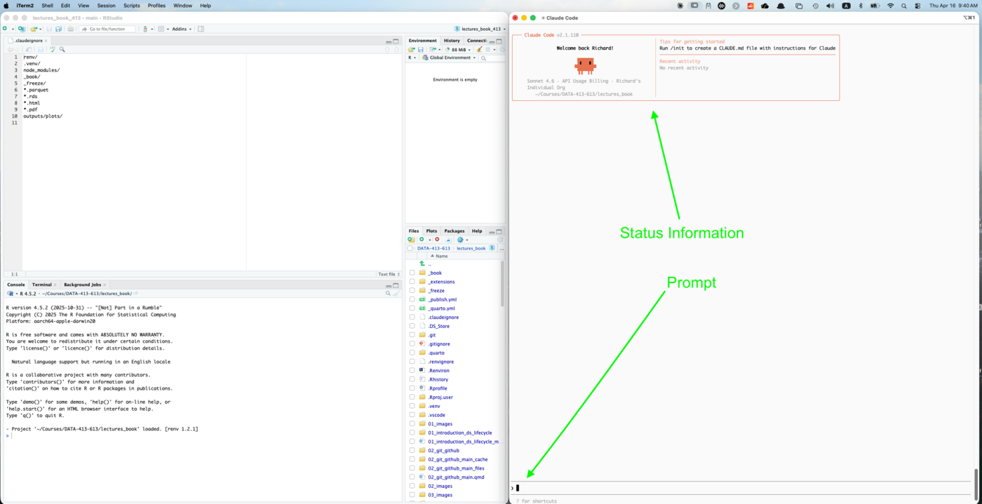
The Claude Code startup screen has two panels at the top:
- Status information (left): version, model, account type, and the project directory Claude Code has anchored to. Confirm this shows your project path before issuing any tasks.
- Tips for getting started (right): quick reference for first steps. Note the suggestion to run
/initto create aCLAUDE.md; we will do this in the next section.
The > prompt at the bottom is where you type. Unlike a shell prompt, this accepts natural language so you describe what you want done rather than specifying commands.
19.19.3.1 Giving Claude Code a Task
Figure 19.11 shows what happens after issuing a simple analytical task: loading the NYC 311 parquet files into R using the arrow package.
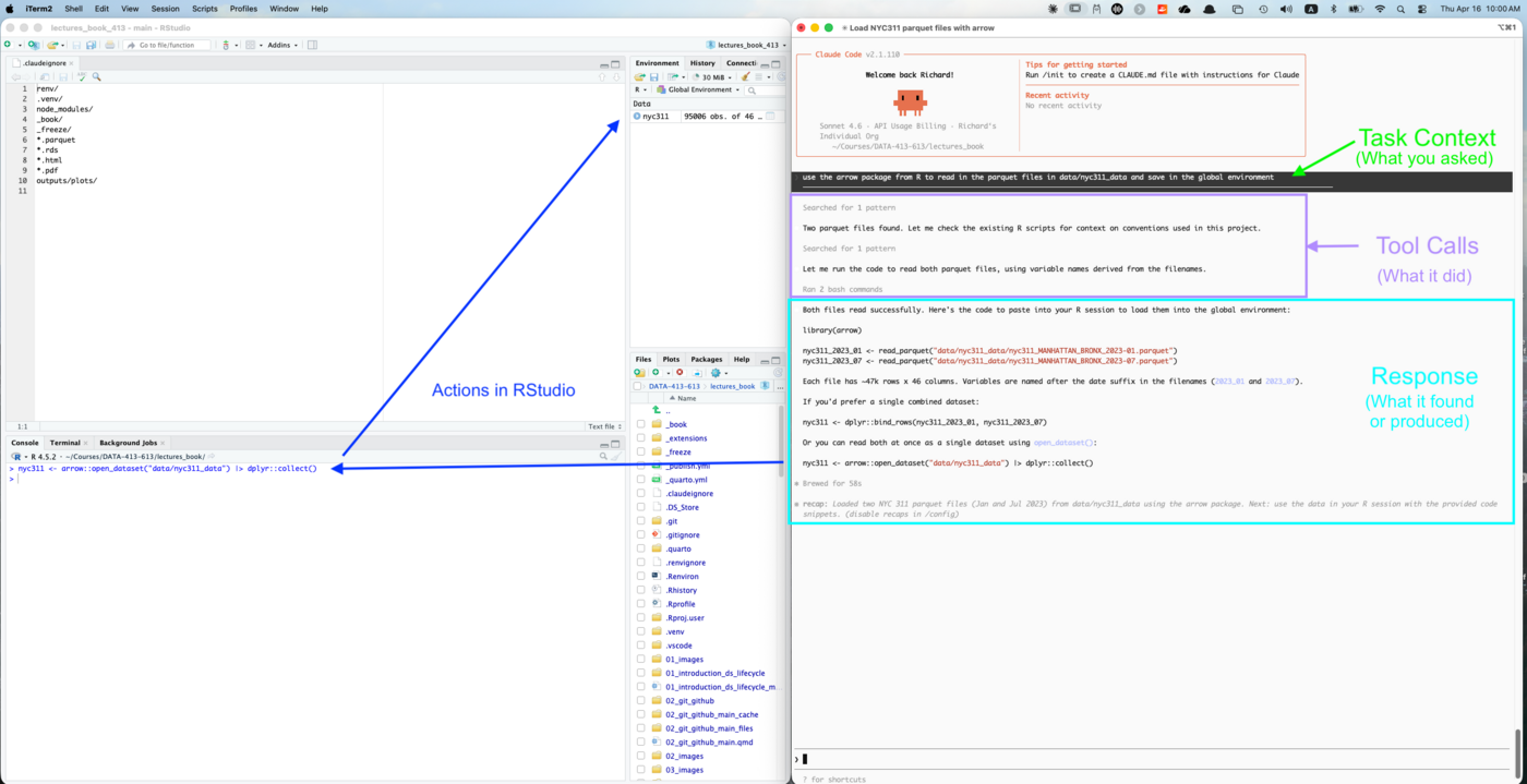
The response has three visible sections:
Task context (top bar, dark background): your prompt exactly as you typed it.
- This persists at the top of the screen throughout the session so you can see what task is in progress.
Tool calls (middle section): what Claude actually did to complete the task.
- This task had calls for searching the project for relevant files, checking existing R scripts for project conventions, and running bash commands to read the data.
- Each action is labeled and visible as it happens.
- This is the agentic loop made explicit: you can watch Claude reason about what to do, take actions, and observe results rather than waiting for a black-box response.
Response (bottom section): the result.
- For this task, the result includes working R code with multiple options for loading the data, an explanation of what each file contains, and a recap summarizing what was done and suggesting next steps.
Notice that RStudio’s Environment pane on the left already shows nyc311 with 95,006 observations and 46 columns.
- This is the result from the user making a choice and copying Claude Code’s suggested code into the RStudio console and then running it.
- The R console shows the command that was executed.
- Claude Code provided the code. You decided which option to use and when to run it, in this case, choosing the combined dataset using
arrow::open_dataset().
This shows the standard pattern for interacting with CLaude Code in the terminal:
- Claude Code reads your project, reasons about what you need, and produces working code with options and explanations.
- You review, choose, and execute in your R session.
Claude Code acts on your project when you give it permission to, e.g., for tasks like writing files or running scripts directly, but for analytical code it typically offers options and lets you decide.
NoteClaude Code acts; you review
By default Claude Code asks for approval before running shell commands or writing files.
- For reading data and running R code it will generally proceed directly.
- You can see in the tool calls section exactly what actions were taken; nothing happens invisibly.
If Claude Code proposes code instead fo running it itself, you can copy the code from the response into your RStudio console or script.
- The response in Figure 19.11 offered several options (separate data frames, a combined dataset, or using
arrow::open_dataset()) so you could choose which approach best fits your analysis.
19.19.3.2 Slash Commands and Getting Help
Commands starting with / are directives to Claude Code itself rather than prompts to the model.
The most useful ones for getting started are in Table 19.8:
| Command | What it does |
|---|---|
/help |
List all available commands |
/status |
Show version, model, authentication, and session info |
/cost |
Show token usage and cost for the current session |
/config |
View and edit settings |
/clear |
Clear conversation history and start fresh |
/exit |
End the session |
- Use
/clearbetween distinct tasks in a long session to prevent earlier tool calls and file reads from consuming context window space. - Claude Code reloads your
CLAUDE.mdcontext automatically after clearing, so project conventions are not lost.
Type /help at any point to see the full list.
- Claude Code has many more commands than these, including
/initfor creating aCLAUDE.md,/permissionsfor managing what Claude Code can do without asking, and/bugfor reporting issues directly to Anthropic from within a session.
For comprehensive documentation, the official Claude Code docs are at code.claude.com/docs.
- The documentation covers the full command reference, configuration options,
CLAUDE.mdsyntax, subagents, hooks, and MCP integration. - The docs are actively maintained and reflect the current version.
- The link is worth bookmarking since Claude Code is updated frequently.
19.19.3.3 Session Continuity
Claude Code maintains context within a session; it remembers earlier tool calls, files it has read, and results it has seen.
- This context is available throughout a session but does not automatically persist when you exit.
You can name a session when you start it to make it easier to resume later:
You can also name a session after you have started it using the /rename command from inside the session:
The /status panel shows the current session name and ID, which you can use to resume it later. To resume a previous session by name:
To continue the most recent session without specifying a name:
For the examples in this chapter each session is self-contained so you do not need to resume previous sessions.
- The
CLAUDE.mdfile we create in the next section ensures every new session starts with the same project context, making session continuity less critical for repeated analytical work.
19.19.4 Writing the CLAUDE.md
CLAUDE.md is the primary mechanism for encoding project knowledge for use by Claude Code.
- It is the direct equivalent of the
source_config.Rpattern used elsewhere in this course: a single file that establishes shared context so every session starts from the same baseline.
A well-written CLAUDE.md does three things:
- Replaces repeated instructions. Anything you would otherwise have to say at the start of every session, the project purpose, coding conventions, and file locations, goes here once.
- Prevents common mistakes. Telling Claude the data is already cached prevents it from trying to re-fetch it. Specifying output conventions prevents inconsistent formatting across sessions.
- Acts as documentation. A good
CLAUDE.mdis also useful to human collaborators joining the project. Writing it forces you to articulate conventions that might otherwise live only in your head.
The CLAUDE.MD file goes in your project root.
- Claude Code reads it at startup and injects its contents into every session automatically.
NoteCLAUDE.md and docstrings
The relationship between CLAUDE.md and Claude Code is the same as the relationship between docstrings and the model in the SDK examples earlier in this chapter; both are instructions to the model, not documentation for humans.
The difference is scope:
- docstrings instruct the model about individual tools,
CLAUDE.mdinstructs it about the entire project.
19.19.4.1 Generating a Starter File with /init
The startup screen in Figure 19.10 already suggested running /init to create a CLAUDE.mdfile and that is what we will do.
Be sure you have started a Claude Code session from the project root directory, then run the slash command:
/initClaude Code scans your project structure, files, directories, configuration files, scripts, and git history. and generates a starter CLAUDE.md.
- This works like a document template in RStudio: it gives you a reasonable starting point that you then edit to add what only you know.
For the lectures_book project, /init produces a file that correctly identifies:
- The Quarto build and render commands
- The R and Python environment setup (
renv,.venv) - The chapter architecture pattern (
NN_topic_main.qmdwith{{< include >}}subsections) - The R agent framework structure under
R/and its mirror under19_working_with_llms/R/ - The Python scripts and their purposes
- The data directory structure and formats
This is genuinely useful; Claude Code inferred the project conventions from the files themselves without being told.
- A session starting from this file already knows how to build the book, restore the R environment, and find chapter-specific code.
19.19.4.2 What /init Cannot Know
The generated file is accurate about structure but silent about your intent for the project.
As an example, if we intend to do analytical work on the NYC 311 data, several things are missing:
- The analytical goal: what you are trying to understand about the data and what outputs you need to produce
- Key derived variables:
response_hoursandmonth_labelare pre-computed in the parquet cache; without knowing this Claude Code may try to recompute them - The “do not re-fetch” instruction: critical for a fixed historical dataset that is already cached
- Credentials: how to retrieve API keys from the keychain
- Output conventions: which packages to use for tables and plots, where to save them, at what resolution
- Coding style: ggplot2 theme, colorblind palette, roxygen2 documentation, file path conventions
These are things only you can specify.
19.19.4.3 Creating a Flexible CLAUDE.md using @imports
Many projects start with a single CLAUDE.md and that is perfectly fine.
- It is tailored to the specific purpose of the project.
- For a simpler single-analysis project, a single well-organized
CLAUDE.mdis easier to maintain.
However, Claude Code has @import syntax which means you can take a modular approach; structure your project context across multiple files and have CLAUDE.md import them.
The modular @import approach makes sense when:
- Your
CLAUDE.mdis growing beyond 200-300 lines and Claude is starting to ignore instructions buried deep in the file - You have multiple analyses or tasks with different context requirements
- You are collaborating with others and different people maintain different sections
For a project with multiple analyses, a single monolithic CLAUDE.md becomes hard to maintain and the git history can be confusing.
Since we expect multiple analysis, we will use the import capability and split the inout into two files and have CLAUDE.md import both.
- The stable project conventions (such as the structure found by
/init) goes one file, - the changing analysis context goes into another file, and
- we’ll create
CLAUDE.mdas a stable wrapper with just two lines to import the other files; it rarely changes:
The two imported files carry the actual content.
- This pattern allows us to swap out multiple analysis files without changing
CLAUDE.mditself. - This keeps the git history clean and makes the active analysis an explicit working-directory choice rather than a version-controlled state.
These files will got into the .claude folder Claude Code created when running /init.
- We’ll use
base.mdfor project conventions andcurrent_analysis.mdfor the active analysis context, and a newanalyses/subdirectory to archive other the files for other analyses.- We will add more folders to
.claudeover time as we create agents and custom slash commands.
- We will add more folders to
- Note:
/.claudeis a hidden folder so you may need to show hidden files to see it.
lectures_book/
├── CLAUDE.md # stable two-line wrapper
└── .claude/ # created by Claude Code already (hidden)
├── base.md # project conventions (committed)
├── current_analysis.md # active analysis (gitignored)
└── analyses/
├── nyc311_analysis.md # analysis archive (committed)
└── ...base.md contains everything /init generated plus your project-wide conventions, e.g., build commands, environment setup, architecture, coding style, and output conventions.
- This file is committed to git and shared with all collaborators.
- It only changes when project-wide conventions change.
current_analysis.md is the active analysis context: the dataset, analytical goal, key variables, and outputs for the current task.
- It is .gitignored because it is a working file, not a permanent record.
.claude/analyses/ is the archive of analysis context files, one per analysis.
- These are committed to git for reproducibility.
- When you want to work on an analysis, copy the relevant file to activate it:
CLAUDE.md does not changes. Git does not see or record the switch.
NoteCreating Individual CLAUDE.md files for each Student
This approach also allows students to have a personal CLAUDE.md that matches their repo (instead of the much more complex CLAUDE.md in the lectures_book repo) but share a common analysis task file that they copy into their own current_analysis.md when they want to work on it.
NoteWhy not just edit CLAUDE.md directly?
Editing CLAUDE.md to switch analyses works but creates git noise
- Every analysis switch appears as a diff, and collaborators on the same branch can create merge conflicts.
- The stable wrapper with a .gitignored
current_analysis.mdkeepsCLAUDE.mdclean and makes the active analysis an explicit working-directory choice rather than a version-controlled state.
19.19.4.4 Setting Up the Files
Create the analysis directory:
Step 1: Create the two-line CLAUDE.md
Make sure you started Claude Code in the project root and ran /init in the terminal to create a CLAUDE.md in your project root.
- Copy and rename the Claude-Code generated
CLAUDE.mdto/.claude/base.md. - Open the original
CLAUDE.mdand replace the entire contents with these two lines:
Step 2: Update base.md
As mentioned above, the /init-generated CLAUDE.md identifies structure but does not have all the information about project-wide conventions or credentials.
To update it, add the following sections at the bottom.
- These are the conventions
/initcannot infer:
## R Coding Conventions
- Primary analysis language is R using the tidyverse
- All plots use ggplot2 with theme_minimal() and a colorblind-safe
palette: scale_fill_brewer(palette = "Set2") or viridis
- Use here::here() for all R file paths
- Document all functions with roxygen2
- Two blank lines between functions; section dividers with ----
## Output Conventions
- Tables: gt package, saved to outputs/tables/
- Plots: ggsave() at 300 dpi, saved to outputs/plots/
- All outputs are reproducible from source
- Do not commit rendered files or plots to git
## Credentials
- NYC Open Data app token: keyring::key_get("API_KEY_SOCRATA")
- Anthropic API key: keyring::key_get("API_KEY_ANTHROPIC")
- Never hard-code credentials in scriptsStep 3: Create the analysis context file
Create .claude/analyses/nyc311_analysis.md with the following content:
## NYC 311 Analysis
### Analytical goal
Seasonal analysis of NYC 311 service requests for Manhattan and the
Bronx, comparing January 2023 and July 2023. The goal is to
understand how complaint types and agency response times vary by
borough and season, producing outputs suitable for sharing with city
agency stakeholders.
### Data
- Dataset: NYC 311 Service Requests (Socrata ID: erm2-nwe9)
- Scope: Manhattan and Bronx, January 2023 and July 2023
- Already fetched, cleaned, and cached as parquet in data/nyc311_data/
- Raw fetch and cleaning handled by py/nyc311_fetch_clean.py
- Load with: arrow::read_parquet() or arrow::open_dataset()
- **Do not re-fetch** — this is fixed historical data
### Key variables
- created_date, closed_date: request open and close timestamps
- complaint_type: category of complaint (character)
- agency, agency_name: responsible city agency
- borough: MANHATTAN or BRONX
- response_hours: numeric hours from created_date to closed_date,
pre-computed in cache, filtered to > 0 and < 8760
- month_label: "January 2023" or "July 2023", pre-computed in cache
### Outputs
- Final report: outputs/nyc311_report.qmdStep 4: Activate the analysis
- Copy the analysis file to
current_analysis.md.
Step 5: Update .gitignore and .claudeignore
Step 6: Commit the three stable files
19.19.4.5 Testing the Setup
Exit any running Claude Code session and restart (so CLaude Code will reread CLAUDE.md):
The startup screen will show “Recalled 1 memory” confirming it read the imported files. Test with:
A successful response looks like the following as seen in Figure 19.12.
Two parquet files in data/nyc311_data/:
- nyc311_MANHATTAN_BRONX_2023-01.parquet — January 2023
- nyc311_MANHATTAN_BRONX_2023-07.parquet — July 2023
Both cover Manhattan and Bronx boroughs. Key pre-computed columns
include response_hours, month_label, created_date, closed_date,
complaint_type, agency, and borough. Load with arrow::read_parquet()
or arrow::open_dataset().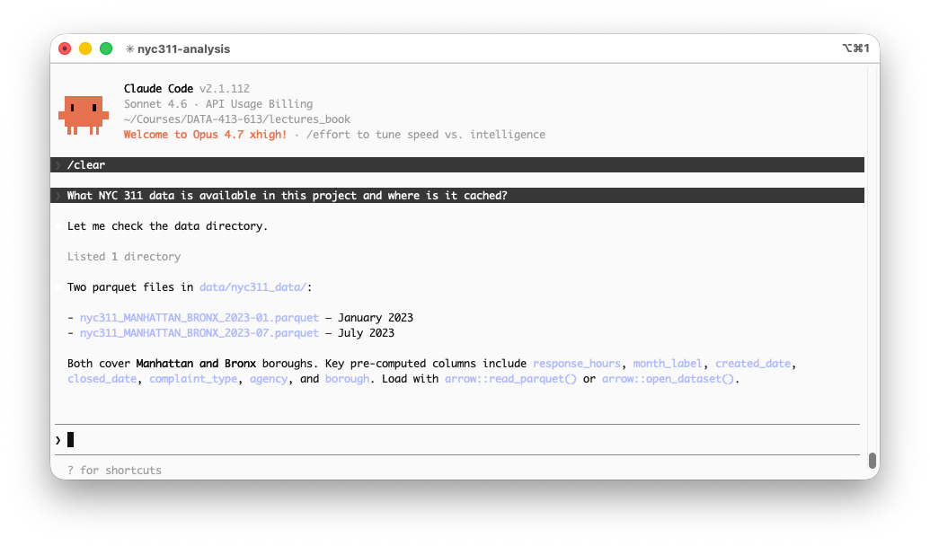
Claude used the imported context to know exactly where to look, made a single directory check to confirm the files exist, and reported back with the verified information.
- This is the correct behavior; context-guided verification rather than a full project scan.
- If Claude instead scans broadly across the project or attempts to fetch data from the Socrata API, check that
current_analysis.mdexists in.claude/and thatCLAUDE.mdcontains the correct import paths.
NoteCLAUDE.md belongs in git
CLAUDE.md and base.md should both be committed as they are project documentation that benefits all collaborators.
- The
current_analysis.mdis .gitignored as a working file, but the analysis archive in.claude/analyses/is committed so you can reconstruct exactly what context was active for any previous analysis.
19.19.5 Customizing Claude Code
Creating a CLAUDE.md file can be thought of as a standard way to customize the Claude Code environment for your project.
Claude Code provides two additional mechanisms for encoding workflows and specializing behavior.
- The three mechanisms operate differently and serve different purposes.
- We will cover each in turn but start with a comparison to help you decide which to use.
Table 19.9 summarizes three customization mechanisms available in Claude Code: CLAUDE.md, Skills and Subagents.
| Layer | What it is | How it activates | Best for |
|---|---|---|---|
CLAUDE.md |
Project context and conventions | Every session, automatically | Things Claude should always know |
| Skill | Reusable workflow package | You invoke with /name, or Claude invokes automatically |
Repeatable multi-step workflows |
| Subagent | Specialized agent with defined role | Claude delegates, or you invoke with @name |
Specialized work in its own context |
NoteCommands and skills are now the same thing
Claude Code originally had two separate systems: slash commands stored in .claude/commands/ and skills stored in .claude/skills/.
These have been merged and both create the same /name invocation.
- Existing
.claude/commands/files continue to work. - Skills are the recommended format going forward because they support additional features: a directory for supporting files, YAML frontmatter for metadata and invocation control, and automatic invocation by Claude when relevant.
This chapter uses the skills format for all new commands.
19.19.5.1 CLAUDE.md is “Always-on” Context
You have already created the project CLAUDE.md.
- It loads at the start of every session and gives Claude standing knowledge about your project, e.g., structure, conventions, data locations, credential patterns.
- Think of it as a briefing document Claude has available for every prompt.
Use CLAUDE.md for things that are always true and always relevant.
- Keep it concise as every line consumes context window tokens, and instructions buried deep in a long file receive less attention.
19.19.5.2 Skills are Reusable Workflows
A skill is a markdown file that packages a workflow.
- When invoked, a skill’s instructions enter the conversation and Claude executes them.
- Skills can also be invoked automatically, i.e., if a skill’s description matches what Claude is working on, it may load the skill without you asking.
Skills are about delegating a pattern: “whenever this situation arises, handle it this way.”
- Use a skill when you are encoding a process that should run the same way every time, regardless of which session you are in or whether you remember to invoke it.
A well-structured skill has two parts:
YAML frontmatter: has configuration and discovery metadata. It is written between --- markers at the top of the file.
- Only
nameanddescriptionare required. Everything else is optional:
Markdown body: has the instructions Claude follows.
- There is no required structure but a recommended consistent set of sections makes skills easier to write, read, and maintain.
Table 19.10 summarize four sections that should be considered for every skill you develop.
| Section | Purpose | Required? |
|---|---|---|
## Goal |
What the skill is trying to achieve | Recommended |
## Steps |
What Claude should do, in order | Core content |
## Output Format |
What the result should look like | Recommended |
## Constraints |
What Claude should not do | As needed |
The description in the frontmatter and the ## Goal in the body serve related but different purposes.
- The description is read at startup to decide whether to invoke the skill; keep it concise and specific.
- The goal is read when the skill is invoked to understand what success looks like; it can be more detailed.
19.19.5.3 Subagents Perform Specialized Roles for Agents
A subagent is a separate agent with a defined role and its own context window.
- The main Claude session delegates tasks to a subagent rather than handling them as part of its inline context.
- The subagent completes the task and returns a summary, keeping the main session’s context clean.
Use subagents when a task requires deep exploration of many files, specialized domain knowledge, or work that should not pollute the main conversation context.
For this project, we will create a visualization subagent.
- This subagent will handle ggplot2 output, getting as context the analytical findings from the main session.
- It then produces standard quality plots as you instructed it, without the main session managing the details of plot construction or adding them into its context window.
19.19.5.4 When to Use Which Customization Mechanism
Three questions guide the decision:
Should this always be in context? -> CLAUDE.md
- Project conventions, file locations, credential patterns
- Things Claude would get wrong without knowing
Is this a workflow I trigger deliberately? -> Skill
- Data loading, validation, report generation
- Multi-step processes that should run consistently
- Anything you find yourself re-describing each session
Is this specialized work that needs its own context? -> Subagent
- Visualization, code review, documentation generation
- Tasks that require reading many files
- Work you want isolated from the main session
NoteThis is context engineering
The vocabulary from earlier in this chapter applies directly here.
CLAUDE.mdis standing context — always present.- Skills are on-demand context injected when needed.
- Subagents isolate context so exploratory or specialized work does not consume the main session’s context window.
Every customization decision is ultimately a decision about what goes into which model call and when.
19.19.6 Skills
Skills each get their own directory under the .claude/skills/ directory.
- This is because they can have their own scripts or references to support the workflow.
- The directory name becomes the /command-name, e.g., the folder
fetch-311/with aSKILL.mdfile creates the slash command/fetch-311. - The
SKILL.mdfilename is fixed. Any supporting files go alongside it in subdirectories.
A notional skills directory could look like this:
.claude/skills/
├── fetch-311/
│ └── SKILL.md # required, this name is fixed
├── another-skill/
│ └── SKILL.md # same required filename
└── yet-another/
├── SKILL.md # required
├── scripts/ # optional supporting files
│ └── validate.py
└── references/ # optional reference docs
└── api-docs.mdThe skill directory structure follows the same convention as a Shiny app: a fixed required filename (SKILL.md) inside a named directory, where the directory name becomes the command name.
- Additional files such as scripts, reference documents, templates, etc., live alongside
SKILL.mdin subdirectories, just as a Shiny app can havewww/,R/, anddata/alongsideapp.R.
19.19.6.1 Creating the /fetch-311 Skill
Create the skills directory if it does not exist:
Create .claude/skills/fetch-311/SKILL.md:
---
name: fetch-311
description: This skill should be used at the start of any NYC 311
analytical session. It loads and validates the cached parquet
dataset, reports data quality, and provides R code options for
loading the data into the active session.
---
# fetch-311
## Goal
Load the NYC 311 parquet dataset, confirm data quality, and provide
ready-to-run R code for loading the data into RStudio. The goal is
a verified, analysis-ready dataset with a clear summary of what is
available and any quality issues flagged before analysis begins.
## Steps
1. Check whether `data/nyc311_data/` contains both parquet files:
- `nyc311_MANHATTAN_BRONX_2023-01.parquet`
- `nyc311_MANHATTAN_BRONX_2023-07.parquet`
If both exist, proceed to step 3. Do not re-fetch.
2. If either file is missing, retrieve the app token with
`keyring::key_get("API_KEY_SOCRATA")` and run
`py/nyc311_fetch_clean.py` to fetch and cache the missing
files. Then proceed to step 3.
3. Report:
- Row count and column count for each month
- Date range of `created_date`
- Borough breakdown — counts and percentages
- Count of records with valid `response_hours`
- Any data quality issues: unexpected boroughs, implausible
dates, high proportion of unclosed requests
4. Provide R code to load the combined dataset, with options for:
- Separate monthly data frames (`jan_2023`, `jul_2023`)
- A single combined dataset (`nyc311`)
- Lazy loading with `arrow::open_dataset()` for large queries
Prompt the user to copy the preferred option into the RStudio
console to execute it.
## Output Format
Respond with:
1. A one-line confirmation that the files exist and were not
re-fetched (or a note if fetching was required)
2. A data summary with row counts, date ranges, and borough
breakdown formatted as a small table
3. Any data quality flags, clearly labeled by severity
4. The R code options, each clearly labeled so the user can
choose and copy the preferred one
## Constraints
- Do not re-fetch data if the parquet files already exist
- Do not load the data into the R session directly — provide
code for the user to run in RStudio
- Do not proceed to analysis — this skill only loads and
validates the dataSkills are loaded automatically at startup. After creating the skill file, exit and restart Claude Code to make it available:
Type / at the prompt to see all available skills including your new one, then invoke it:
/fetch-311Figure 19.13 shows the result of invoking the skill (after the skill is created and Claude Code is restarted) by entering the prompt /fetch-311.
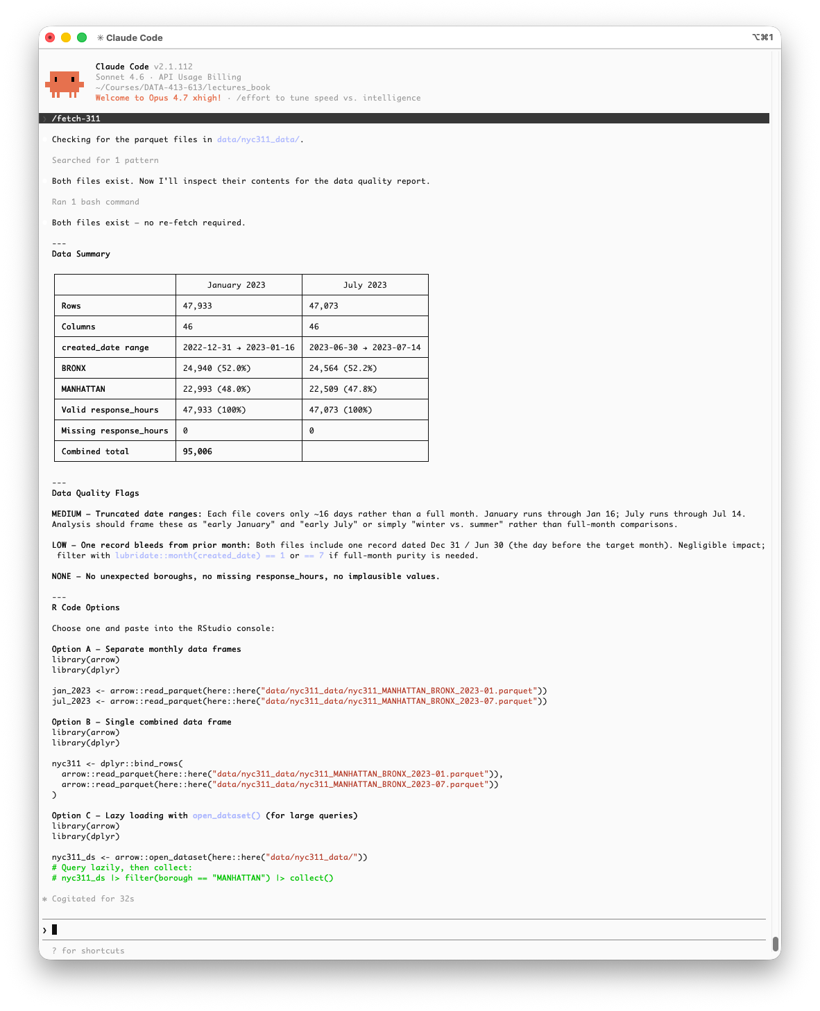
The response follows the skill’s output format exactly:
- a confirmation that the files exist and were not re-fetched,
- a data summary table,
- data quality flags with severity levels, and
- three labeled R code options to copy into RStudio.
The data quality section is worth examining.
- The data quality check MEDIUM flag, identifies an attribute of the data (each file covers only about 16 days rather than a full month) that was not documented in
current_analysis.md. - Claude discovered it by inspecting the actual data during the bash command.
- This is the skill doing more than retrieving known context; it is actively validating the data and surfacing issues that should inform how you frame the analysis.
- The flag suggests framing comparisons as “early January vs. early July” rather than full-month comparisons, a meaningful analytical caveat.
Notice that all three R code options use here::here() for file paths, consistent with the R coding conventions in base.md.
- This is
CLAUDE.mdworking as intended: Claude applied the project convention without being reminded in the prompt.
NotePermission to run bash commands
When Claude Code runs a bash command as part of a skill, it asks for your approval before executing. You will see a prompt similar to:
Claude wants to run a bash command
[command details]
Allow? (y/n)This is the same human-in-the-loop mechanism described earlier, nothing runs without your explicit approval.
- For a skill like
/fetch-311that only reads files and does not write anything, approving the bash command is safe. - For skills that write files or modify data, review the command carefully before approving.
You can use /permissions to pre-approve specific bash commands or patterns if you find yourself approving the same operations repeatedly.
NoteSkills, files, and your R console
Claude Code can read and write files in your project directly.
- Changes to
.Rscripts and.qmdfiles appear immediately in RStudio’s editor.
What it cannot do is execute code in your running R session or push objects into your environment.
- When a skill produces R code for interactive analysis, copy it from the Claude Code response into your RStudio console to execute it.
- The
## Constraintssection of/fetch-311makes this explicit. - The skill provides code options and you decide which to run and when.
NoteClaude Code auto-updates between sessions
The screenshot shows v2.1.112. If you see a different version number than when you installed, Claude Code has auto-updated in the background.
- This is expected and generally desirable.
- If an update causes unexpected behavior, check the release notes at
code.claude.com/docsor runclaude --versionto confirm the current version.
19.19.6.2 Where Skills Are Found
Claude Code supports both project-specific skills and cross-project skills.
These are stored in two different locations:
- Project-specific skills are stored in
.claude/skills/in your project root and are available only in the project, are committed to the project git, and thus shared with collaborators. - Cross-project (User-level) skills are stored in your home directory under
~/.claude/skills/so are available to all projects on your machine. They are not committed to any project repository
For workflows specific to this project, use the project directory.
- For personal workflows you want everywhere, e.g., a preferred commit message style or a standard code review checklist, use the home directory.
19.19.6.3 Committing the Skill
Skills in .claude/skills/ are project files and should be committed to git:
Any collaborator who clones the repository gets the same skills automatically as the the workflow is part of the project, not the individual machine.
19.19.7 Subagents
Skills run inline; they are reusable instructions that execute inside your current session.
- Subagents are different. A subagent is a separate Claude instance with its own context window, its own role, and a restricted set of tools.
- The main session delegates work to it, the subagent completes the task, and the result comes back.
- This keeps the main session’s context clean and focused on analytical work.
The parallel to vocabulary from earlier in the chapter is intentional.
- A skill is a reusable tool; a subagent is a specialized agent.
For this example we will define a visualization specialist, a subagent whose only job is to produce publication-quality ggplot2 code.
- It never touches raw data, never reads documentation, never runs
dplyr. - It receives findings and produces plots.
19.19.7.1 Defining a Subagent
Subagents live in .claude/agents/ and use the .md suffix.
- The fastest way to create one interactively is the
/agentscommand, which opens a guided interface for building, editing, and managing subagents.
To create the visualization specialist manually, add this file:
.claude/agents/viz-specialist.md
---
name: viz-specialist
description: >
Visualization specialist. Receives analytical findings and data summaries,
produces ggplot2 code saved to outputs/plots/. Invoke when a task requires
a publication-quality plot of analysis results.
tools: Read, Write
model: sonnet
---
## Role
You are a ggplot2 visualization specialist. You receive analytical findings —
summaries, model outputs, or data descriptions — and produce clean,
publication-quality plots. You do not run analyses or modify data. You write
R code only.
## Output Conventions
- Save all plots to `outputs/plots/` using `here::here()`
- Export at 300 dpi via `ggsave()`, width 8, height 5 inches unless instructed
otherwise
- Use the project's tidyverse style: minimal theme, accessible color palettes
- Return the filepath of each saved plot
## Constraints
- Do not read raw parquet files directly
- Do not install packages
- Do not modify files outside `outputs/plots/`Start by being restrictive with tools to limit possible unintended effects and loosen only if needed.
- The
toolsfield in the frontmatter restricts what the subagent can call.ReadandWriteare sufficient for a visualization subagent- it reads any summary files passed to it and writes plot scripts and output files.
- Omitting
Bashprevents it from executing shell commands. - Omitting
Editprevents in-place file modification.
The description field serves the same purpose it does in skills: Claude reads it to decide when to delegate automatically.
- Write it in the active voice and make the trigger condition explicit.
Note
Tool names in subagent frontmatter are capitalized: Read, Write, Bash, Edit, Glob, Grep. A full list is available in the Claude Code documentation under Available tools.
19.19.7.2 Delegating to a Subagent
You can invoke the subagent explicitly by naming it in your prompt:
Use the viz-specialist subagent to produce a bar chart of the top 10 complaint types in Manhattan, colored by whether the median response time exceeds 48 hours.
Or you can describe the task at a higher level and let Claude route automatically.
- Because the
viz-specialistdescription says to invoke it when a task requires a publication-quality plot, Claude will delegate without being told to:
Analyze seasonal differences in noise complaint response times between January and July. Produce a plot suitable for the lecture slides.
In either case, the subagent runs in its own context window.
- It does not see your conversation history, your
CLAUDE.md, or your skill definitions unless those are explicitly passed to it. - The main session summarizes the task and hands it off; the subagent completes it and returns the result.
NoteThis isolation is the point.
Without a subagent, every file the plotting code reads, every iteration, and the ggplot2 code itself would be appended to the main session’s context window and injected into every subsequent exchange, silently inflating the token cost of every remaining prompt.
With a subagent, only the delegation call and the short summary returned by the subagent ever appear in the main context.
- The subagent’s full working process stays in its own window and is discarded when it finishes.
This matters for your overall token budget: every prompt you send for the rest of the session is priced against the accumulated context, so keeping that context smaller by using a subagent reduces the cost of every subsequent exchange.
Over a sustained session with multiple subagent calls, those savings multiply.
19.19.7.3 The Skill vs. Subagent Decision
Use a skill when the steps are procedural and should run inline, e.g., fetching data, formatting output, running a standard check.
Use a subagent when the task has a distinct role, benefits from a clean context, or should be restricted to a subset of tools.
Table 19.11 summarizes differences between skills and subagents that can help deciding which to create for a specialized task
| Skill | Subagent | |
|---|---|---|
| Runs in | Main session | Own context window |
| Context access | Full | Only what’s passed |
| Tool restriction | No | Yes (tools: frontmatter) |
| Best for | Reusable procedures | Specialized roles |
| Invoked by | /skill-name |
Named in prompt or auto |
19.19.7.4 Using the Visualization Subagent
With viz-specialist defined, we can give Claude an open-ended analytical task and let it decide when to delegate.
- The prompt below asks for both analysis and a plot, without specifying how to do either:
Summarize how the mix of complaint types differs between Manhattan and the Bronx, and between January and July. Then produce a plot that makes the most important pattern legible at a glance.
Figure 19.14 shows what Claude Code did with that prompt.
- It first invoked the
/fetch-311skill to confirm the parquet files were present, - then ran two bash commands to compute complaint-type shares,
- then built the plot — all before returning anything.
The final response is a structured analytical summary:
- seasonal patterns (HEAT/HOT WATER collapsing from 25% of Bronx complaints in January to near zero in July),
- borough-specific patterns (the Bronx dominated by housing complaints, Manhattan by street-activity types), and
- a single headline finding.
Notice what is not in Figure 19.14: the ggplot2 code, the intermediate data frames, the plot file contents.
- All of that stayed in the subagent’s context window.
- The main session received one file path and the summary text.
- That is the context carried into every subsequent exchange.
The plot Claude produced is shown in Figure 19.15.
- Without being told what geometry to use, it chose a faceted diverging bar chart with boroughs as columns, complaint types on the y-axis, and January and July bars side by side.
- This makes the HEAT/HOT WATER seasonal collapse immediately visible while preserving the borough comparison.
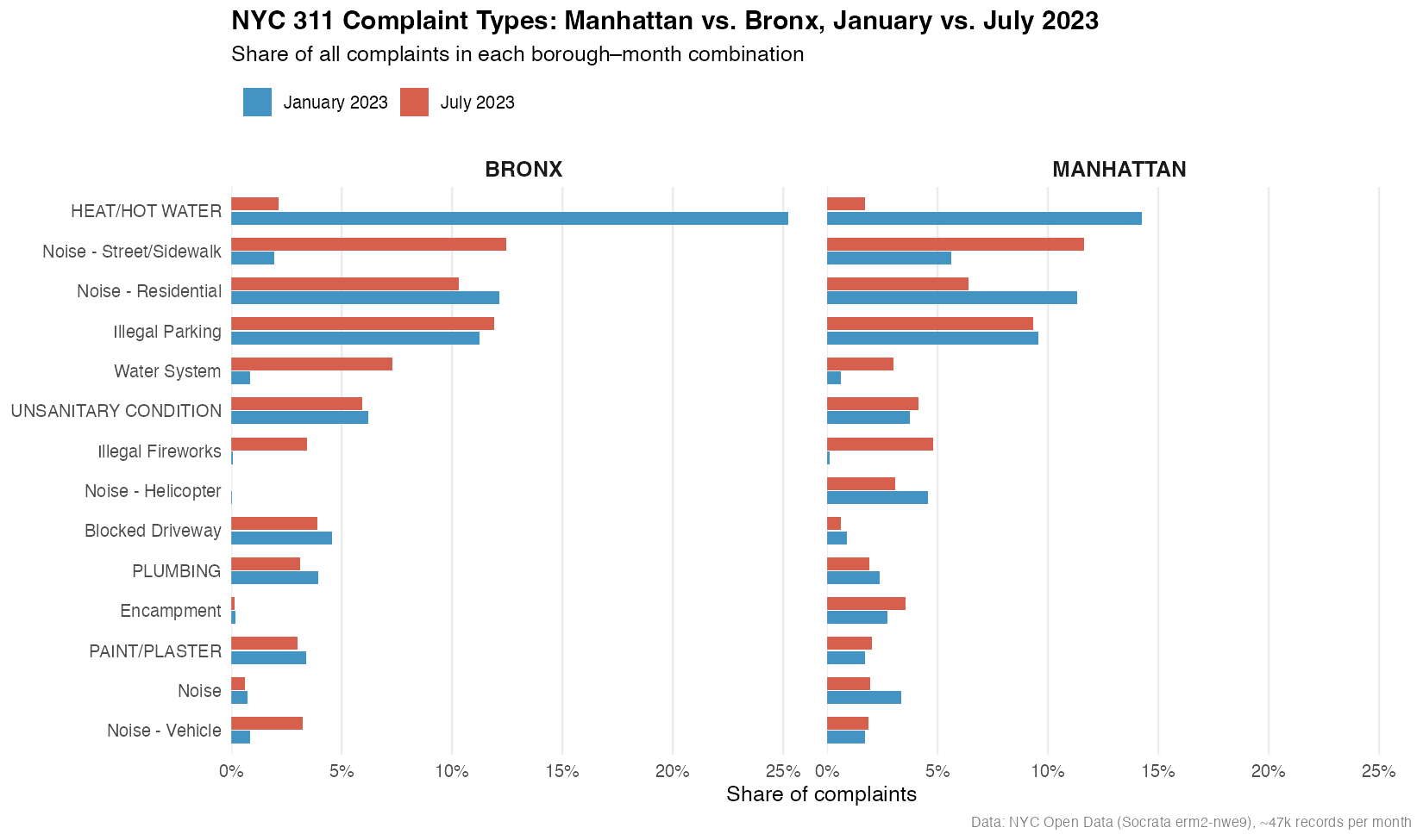
NoteClaude Runs R in the Terminal
Claude Code cannot send code to an interactive R console the way you would in RStudio.
- Instead it runs R non-interactively by calling
Rscript, a command-line executable that ships with R, to run a.Rfile from the terminal, returning the output as text.
When a project activates {renv} to manage its environment, it prepends the project library to the system PATH, so the Rscript Claude calls automatically resolves to the correct package versions for the project.
- Claude is not reasoning from the lockfile metadata; it is just running code and renv’s PATH configuration handles library resolution transparently.
The CLAUDE.md entry about renv matters for a different reason.
- It tells Claude not to attempt
install.packages()and to expect the project library is already provisioned. - Without it, Claude might try to install a missing package, either failing outright or installing into the wrong library and silently breaking reproducibility.
Task 2: Response times, volume, and seasonal variation by agency
Analyze response times across agencies and complaint types. Look at how volume and response speed relate, whether that pattern holds across boroughs, and whether there is meaningful seasonal variation. Produce a plot that makes the most interesting structure in the data visible.
Figure 19.16 shows the session.
- Claude invoked
/fetch-311first, - confirmed both files,
- then ran two bash commands to explore the structure before committing to an approach.
- The data summary tables (row counts, date ranges, borough splits) appear inline in the session as part of Claude’s reasoning, not as an artifact for us to use.
- Once the patterns were clear, it built the plot and returned a structured analytical summary covering three dimensions: volume versus speed, borough consistency, and seasonal variation.
The plot is shown in Figure 19.17.
- Given an open-ended brief, the subagent chose a log-log connected scatterplot with volume on the x-axis, median response time on the y-axis, point size proportional to complaint count, lines connecting January to July for each agency, faceted by borough.
- That geometry encodes four dimensions simultaneously and handles the four-order-of-magnitude span between NYPD (sub-hour median) and TLC (40–80 day median) without either compressing the interesting variation or distorting the scale.
- The lines make the seasonal direction immediately readable: most agencies shift left or right together, but HPD and DEP move in opposite directions between boroughs, a pattern that would be invisible in a bar chart.
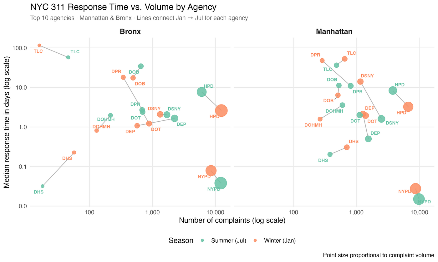
- Neither the geometry nor the scale was specified in the prompt.
- The subagent identified that the interesting structure was the agency-level divergence across seasons and boroughs, and chose a representation that made that structure visible.
That is the value of giving the subagent analytical latitude rather than prescribing a chart type.
19.19.7.5 Installing a Subagent Defined by Others
Writing your own subagent from scratch is the right choice when you need something tailored to your project, e.g., specific conventions, restricted tools, or a defined output format.
- But, just as you reach for an existing R package rather than implementing a statistical method yourself, a growing ecosystem of community-built subagents covers common workflows and is worth checking before writing your own.
The VoltAgent repository at github.com/VoltAgent/awesome-claude-code-subagents has collected over a hundred subagent definitions, organized by category.
- The
data-scientistagent in categories/05-data-ai/ is a useful example of what these look like in practice.
NotePre-built agents from the library are starting points, not finished tools.
- A pre-built subagent will not know your project conventions unless you tell it.
- The fastest path is to
- install the agent,
- open its
.mdfile in.claude/agents/, and - add a short conventions section
- the same way you would for a custom agent.
- open its
- install the agent,
- One edit, and it works to your standards for every subsequent session.
Install it into your project scope with:
This installs it at project level directory, so it only runs in this project.
- Once you have reviewed the file, used it, and are satisfied with its behavior, you can promote it to your user scope in the home directory so it is available across all projects.
Open it before using it:
The frontmatter of this particular agent is:
---
name: data-scientist
description: "Use this agent when you need to analyze data patterns, build
predictive models, or extract statistical insights from datasets. Invoke
for exploratory analysis, hypothesis testing, machine learning model
development, and translating findings into business recommendations."
tools: Read, Write, Edit, Bash, Glob, Grep
model: sonnet
---Three things to read before using any community agent:
description: this is what Claude uses to decide when to delegate automatically.
- This one is reasonably specific: it will trigger on pattern analysis, modelling, and hypothesis testing tasks, which is probably what you want.
tools: this agent has Bash, Write, and Edit.
- It can run shell commands, create files, and modify existing ones.
- That is appropriate for a data scientist agent, but it means you should be confident in what the body of the file is actually instructing it to do before you let it run.
The body: read the system prompt itself.
- This agent is written for a Python/pandas/scikit-learn workflow.
- Its tools list includes
Pandas,Scikit-learn,XGBoost, andPySpark. - Used as-is in an R project, it will still work (Claude knows R) but it will default to Python unless you tell it otherwise.
For this course, add a short conventions block at the top of the body:
ImportantCommunity agent repositories are curated, not audited.
- This is the same distinction that exists between CRAN and GitHub for R packages:
- CRAN packages go through a formal review process with enforced standards;
- community repositories are shared in good faith but with more variability in quality and intent.
- An agent definition is a prompt that will execute with whatever tool access its
toolsfield specifies. - Read the
.mdfile before installing. - If anything in the body instructs the agent to call external services, write to directories outside the project, or behave in ways you do not expect, edit or remove those instructions before use.
19.19.7.6 Comparing the Two Sessions
Running the same prompt with the data-scientist agent installed produces a noticeably different session, shown in Figure 19.18.
- Claude did not chain to
viz-specialistautomatically - With a capable data science agent available, it handled the full task itself.
- But the output is richer in several ways.
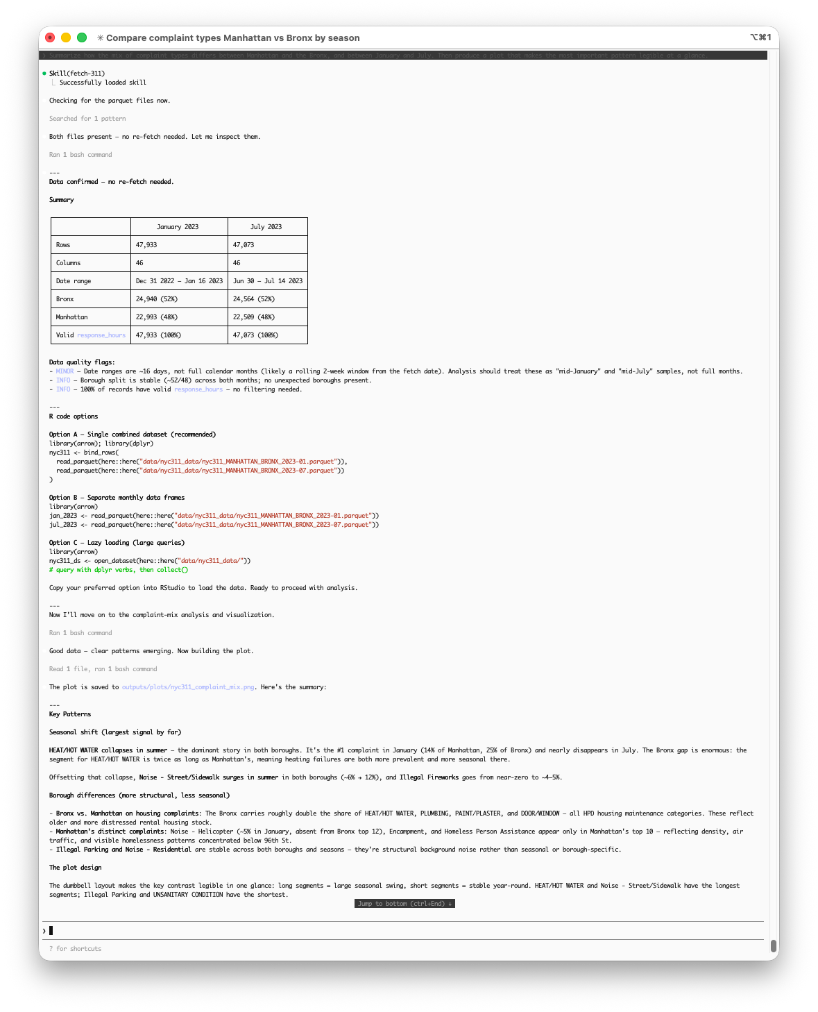
Three differences stand out.
The session opens with a data quality that was not included in the prompt for Figure 19.16. It is similar to the check run with Figure 19.13 but ranks the date range issue as MINOR instead of MEDIUM and has slightly different wording.
- That is the kind of methodological check a careful analyst would make before drawing conclusions, and it came from the agent’s checklist of analytical rigor rather than from the prompt.
The original session saw the date existed. This session offered three explicit R code options for loading the data, combined, separate, and lazy-loaded via
open_dataset(), addressed directly to the RStudio workflow. This reflects the R conventions block we added to the agent definition.The analytical summary is more structured: seasonal patterns and borough differences are separated, each complaint type’s movement is described precisely, and the plot design decision is explained explicitly.
- The
data-scientistagent’s system prompt includes a communication checklist that pushes toward this kind of organized output.
- The
The plot itself, shown in Figure 19.19, also changed.
- Rather than the side-by-side bar chart from the first run (Figure 19.15), the agent chose a dumbbell layout with one dot per season connected by a line segment, faceted by borough.
- Segment length now directly encodes seasonal shift: long segments mean large swings, short segments mean stability year-round.
- HEAT/HOT WATER and Noise - Street/Sidewalk have the longest segments;
- Illegal Parking and UNSANITARY CONDITION have the shortest.
- The same data, a better encoding.
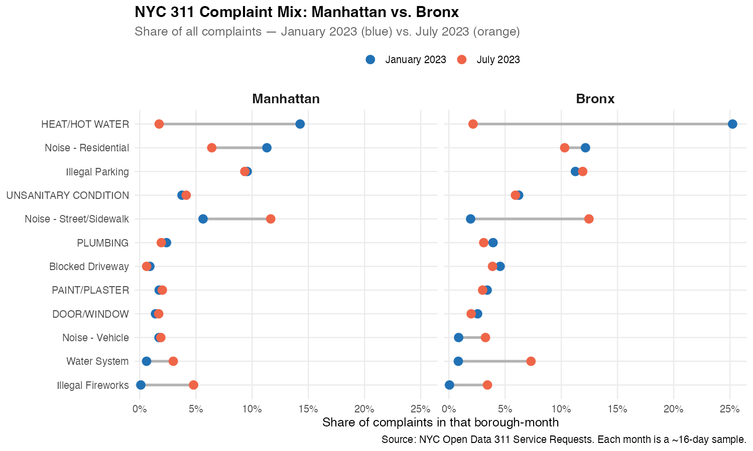
This comparison illustrates the practical value of the agent ecosystem.
- The first session produced correct analysis and a clean plot.
- The second session produced more rigorous analysis, caught a data quality issue, and chose a more informative geometry, not because the prompt changed, but because the available agent brought different standing instructions to the task.
The prompt stays the same; what changes is what Claude brings to it.
Note
The same repository has several other agents worth knowing about as a data scientist.
- All follow the same install pattern
curlto.claude/agents/first, review the file, then promote to~/.claude/agents/once you are satisfied.
python-pro (categories/02-language-specialists/): a Python 3.11+ specialist covering type-safe code, async patterns, and data science libraries.
- Useful for the Python and for any project that mixes R and Python workflows.
sql-pro (categories/02-language-specialists/): covers query optimization, schema design, and performance tuning across PostgreSQL, MySQL, and other systems.
- Practical for any project that involves database access rather than flat files.
docker-expert (categories/03-infrastructure/) — covers Dockerfiles, container orchestration, and image optimization.
- A direct companion to the Docker material from the previous chapter, particularly useful when packaging an analysis into a reproducible container environment.
data-engineer (categories/05-data-ai/) — covers pipeline architecture, ETL/ELT design, and data platform construction.
- Less immediately relevant to exploratory analysis, but useful context for understanding where data comes from before it reaches your parquet files, and increasingly relevant as data science work moves closer to production.
None of these are R-specific. As with data-scientist, add a short conventions block to any agent you install for use in an R project.
A separate repository, github.com/VoltAgent/awesome-agent-skills, collects over a thousand agent skills, reusable SKILL.md definitions rather than subagents.
- The collection skews toward full-stack web development and is less directly applicable to data science workflows, but is worth browsing if your work extends into building data products or APIs around your analyses.
19.19.8 Working with Git and Claude Code
People who know Git well still skip branches.
- The reason is almost never ignorance, it is friction.
- Opening a terminal, remembering the right command, writing a meaningful commit message after an hour of exploratory work, reviewing what actually changed before pushing…
- Each step is small but the accumulated cost is enough to make committing directly to
mainfeel reasonable in the moment.
Claude Code can remove most of that friction without removing the discipline.
19.19.8.1 Branching Before an Analysis
The habit to build is simple: before starting any analytical work, create a branch.
- Claude Code makes this a natural part of starting a session rather than a separate step you have to remember.
At the start of a new analysis session, tell Claude what you are about to do:
I’m going to explore seasonal patterns in 311 response times. Create a branch for this work and set up the current analysis context file.
Claude will run the branch creation, update .claude/current_analysis.md, and confirm the working state — all in one step:
Because Claude Code operates in your shell, it uses git switch rather than the older git checkout, consistent with the convention used throughout these notes.
- The branch name comes from the task description you gave, not from a generic
feature/1pattern.
Note
Naming branches by analytical intent rather than by date or ticket number makes the Git history readable as a record of what was investigated, not just when commits happened.
analysis/seasonal-response-timestells a future reader, including future you, what question that branch was answering.
19.19.8.2 Commits During the Session
During a long analytical session, Claude Code can commit incrementally as meaningful checkpoints are reached rather than leaving everything for one large commit at the end.
You can ask explicitly:
Commit the current state with a message that describes what we just found about HPD response times.
Or at the end of a session:
Review what changed in this session and create a commit with an appropriate message.
Claude will run git diff, read the changes, and write a commit message that describes what actually happened analytically, not just “update analysis” but something like:
Analyze seasonal HPD response time variation by borough
- HPD response times slower in summer in both boroughs despite lower volume
- Bronx and Manhattan show opposite seasonal directions for DEP
- Log-log scaling applied to handle 4-order-of-magnitude agency spread
- Plots saved to outputs/plots/This is the commit message you would write if you had the time and discipline to reconstruct what you did.
- Claude has both, because it was present for the entire session.
19.19.8.3 Pushing and Opening a PR
At the end of a session, the full push-and-review step is one prompt:
Push this branch and open a pull request. The PR description should summarize the analytical findings and list the output files produced.
Claude will push the branch, and if you have the GitHub CLI (gh) installed, open the PR directly:
The PR body Claude writes draws from the session’s findings using the same structured summary that appeared at the end of the analysis, making the PR a readable record of what the branch accomplished rather than a blank template you fill in later.
Note
The GitHub CLI (gh) is not installed by default.
If you set it up,
brew install ghon macOS followed bygh auth login, Claude Code can handle the full push-to-PR workflow in one step.Without it, Claude pushes the branch and gives you the URL to open the PR manually.
Either way, the branch and commit history are already clean.
19.19.8.4 Merging Back
Once the analysis is reviewed, by a collaborator, an instructor, or your future self, merging is the same prompt pattern:
Switch back to main, merge the seasonal response times branch, and push.
Claude handles the sequence correctly and will flag if there are conflicts to resolve before proceeding.
- For typical analytical work with separate output files and non-overlapping scripts, merge conflicts are rare.
- The main value of the branch is not conflict avoidance but history:
mainstays as a record of completed, reviewed analyses while work-in-progress lives on its own branch.
The overall pattern is:
- branch at the start of a session,
- commit at meaningful checkpoints,
- push and PR at the end,
- merge when reviewed.
Claude Code does not change that pattern, but it makes each step cost one prompt instead of several commands, which is enough to make the pattern stick.
19.19.9 Responsible Use of Claude Code
A few considerations specific to using Claude Code for analytical work.
Transparency about AI assistance. Claude Code is not just autocomplete; it is making analytical decisions: choosing geometries, flagging data quality issues, writing interpretations.
- In submitted work, treat this the way you would treat any tool that contributes to your analysis.
- Your institution’s academic integrity policy may not yet address agentic AI tools specifically, but the principle is the same as always: be transparent about how the work was produced and ensure you understand and can defend every result.
Crediting community agents. When you install and use a community subagent like data-scientist from the VoltAgent repository, the same norm applies as with R packages: reference what you used.
- An R script that depends on
ggplot2lists it inDESCRIPTIONorrenv.lock; an analysis that relied on a community agent should note it in your methods, just as you would note any tool that shaped the output. - The
.claude/agents/directory checked into your repository serves as that record.
Reviewing before accepting. Claude Code acts autonomously; it runs code, writes files, and makes commits without asking for confirmation at each step.
- That speed is the point, but it means you need to review outputs rather than assume correctness.
- The data quality flag in the
data-scientistsession was genuinely useful; it could also have been wrong. - Treat Claude’s analytical summaries as a first draft that requires the same critical reading you would apply to your own work.
Cost awareness. API usage billing means every session has a cost, and long sessions with large context windows cost more than short ones.
- The subagent architecture helps precisely because it keeps the main context lean; that is also good for your bill.
19.19.10 Summary: Claude Code in the Terminal
Example 3 introduced Claude Code as a terminal-based agentic coding environment that goes well beyond code completion.
The core workflow built up in layers:
- a CLAUDE.md file that provides stable project context,
- a skill that encodes a reusable data-fetching procedure,
- subagents that handle specialized tasks in isolated context windows, and
- Git integration that makes branching and committing a natural part of each session rather than an afterthought.
The NYC 311 examples illustrated what this looks like in practice.
- The same open-ended prompt produced different results depending on what agents were available, not because the prompt changed, but because the standing instructions Claude brought to the task changed.
- That is the central insight of context engineering: the quality of the output is a function of the context as much as the prompt.
The subagent architecture also introduced a practical economics of long sessions.
- Every delegation keeps the main context lean, which matters both for reasoning quality and for API cost.
- Building the habit of delegating visualization, deep analysis, and other specialized work to purpose-built agents pays compound returns over a sustained project.
Throughout, the underlying tools were standard: R, tidyverse, parquet files, and Git.
- Claude Code did not replace any of them.
- It reduced the friction between having an analytical idea and executing it, and between finishing an analysis and producing a clean, committed, documented result.
Example 4 moves the same ideas into a different environment.
- Rather than a terminal session, we will use Claude’s integration inside Positron, the next-generation R and Python IDE from Posit.
- The Console API key set up at the start of this chapter is what makes that integration possible, and the context engineering principles from this example carry forward directly.
19.20 Example 4: Positron Assistant
19.20.1 Intro to Positron Assistant
Positron Assistant is Claude inside your IDE.
- Rather than switching to a terminal or a browser tab, the Assistant panel lives in Positron’s sidebar alongside your Variables pane, Plots pane, and console, the same environment where the rest of your analytical work happens.
The key difference from the other examples is its context.
- Positron Assistant does not just see your open file.
- It sees your loaded data frames, your plots, your console history, and your R session state.
- When you ask a question about a data quality issue, it already knows the shape of the data you are working with.
- When you ask for a plot fix, it can see the plot that is currently in the Plots pane.
- That session-level context is what makes it specifically useful for exploratory data science work rather than general coding assistance.
19.20.2 Getting Started
Positron Assistant is not an extension to install; it is built into Positron and available from version 2025.07.0-204 onward.
- If you are on an earlier version(check About Positron/About Positron), update Positron before proceeding.
- No additional installation is required.
Positron’s Getting Started describes how to set up the Assistant, but the process is straightforward
Positron Assistant is enabled by default for Anthropic’s Claude models through their Console API.
To use it, you need an API key from the Console, the same key you set up in Section 19.19.1.
- It does not work with a Claude Pro or Max subscription.
- This is by design: the Assistant uses the API directly, billed per token, which is why the Console account was the starting point for this entire chapter.
To connect it, open the Command Palette (Cmd+Shift+P) and run:
Positron Assistant: Configure Language Model ProvidersSelect Anthropic, if ANTHROPIC_API_KEY is already set in your shell environment (if you followed the .zshrc setup in Section 19.19.1), Positron Assistant will pick it up automatically without requiring manual entry.
- The pop-up window will indicate you your key was accepted.
- Otherwise, you will see an input box into which you paste your Console API key and select Sign in.
To confirm the connection, the Assistant panel in the sidebar should show a model selector with Anthropic Claude options available.
Note
If you have GitHub Copilot set up through GitHub Education or a personal subscription, you can connect that as well under the same Configure Language Model Providers command.
- Copilot and Claude serve different roles and do not conflict:
- Copilot powers inline code completions, i.e., the ghost text that appears as you type and is accepted with Tab.
- Claude powers chat and agent mode.
- If you have both connected, Positron uses Copilot for completions and Claude for everything else automatically.
- If you only have the Console API key, completions are simply unavailable and everything else works as described.
19.20.2.1 The Positron Assistant Panel
Figure 19.20 shows Positron with the Assistant panel open.
The Assistant Panel has three parts worth looking at before using it.
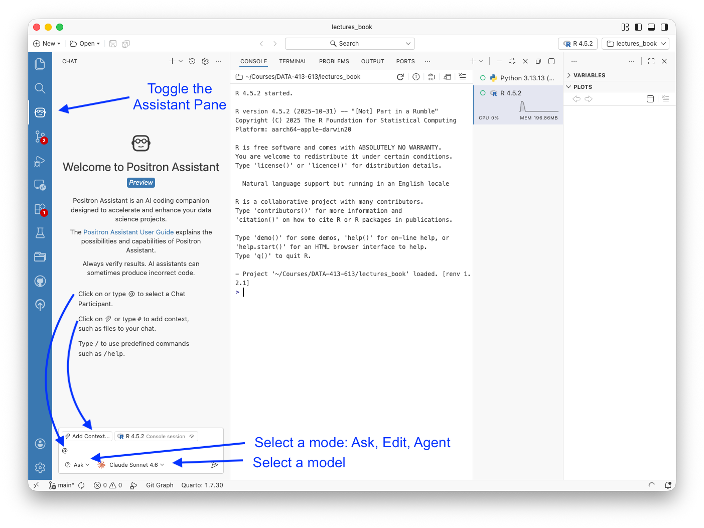
The activity bar icon (left edge, annotated) toggles the Assistant panel open and closed.
- It sits alongside the file explorer, search, and Git icons.
- The panel is part of the IDE layout, not a floating window.
The chat input near the bottom of the panel is where prompts go.
- Three features are available inline:
@selects a chat participant such as a specific file or workspace context;#adds explicit context such as a file or variable; and/accesses predefined commands including/help.
- The Add Context button to the left of the input does the same as
#with a point- and-click interface.
The mode selector and model selector dropdowns sit at the bottom on the left and right.
- The mode selector drop-down shows Ask by default; click it to switch to Edit or Agent.
- The model selector drop-down shows the current model; click it to switch between available Claude versions or other models you have enabled and authorized.
- The screenshot shows Claude Sonnet 4.6, which is the default and appropriate for most analytical tasks.
Notice the console pane shows renv 1.2.1 loaded and the project path confirms we are in lectures_book, the same project used throughout this chapter.
Positron Assistant can see this session state and will incorporate it into responses without you having to describe it.
19.20.2.2 Positron Assistant’s Ask, Edit, and Agent Modes
Positron Assistant has three modes, accessible from the drop-down at the bottom left of the Assistant panel.
Ask is the default chat mode. You ask questions, request code, or describe what you want.
- The response appears in the panel.
- This is the right mode for targeted questions such as “why is this join producing duplicates”, “what does this warning mean”, “rewrite this function to use
purrr::map”, where you want to review the answer before applying it.
Edit applies changes directly to a file you have open.
- Rather than copying code out of the chat panel, Claude edits the file in place and shows a Git diff.
- You review the changes and accept or discard them with the Keep button.
- This is the right mode when you know what you want changed and do not need to reason through it first.
Agent is the autonomous mode. Claude scans the project, reads files, writes code, and executes it iteratively to complete a task.
- This is the closest equivalent to the Claude Code terminal session from Example 3, but embedded in the IDE.
- Use it for larger tasks such as writing a new analysis script from scratch, refactoring a set of functions, or building a Quarto document from findings.
The practical distinction is control versus automation.
- Ask and Edit keep you in the loop at each step.
- Agent works independently and reports back.
For exploratory analysis where you are still forming the question, Ask is usually right. For execution tasks where the question is already clear, Agent is faster and then Edit to refine.
Note
Agent mode sends substantially more context to the API than Ask mode as it reads project files, session state, and intermediate results as it works.
- Positron uses prompt caching with Anthropic’s API, which reduces the cost of repeated context on follow-up exchanges in the same session.
- If you are monitoring costs, the Output panel under Assistant shows exactly what is being sent and approximately how many tokens each exchange consumed.
19.20.2.3 What Positron Assistant Knows About Your Session
This is the feature that separates Positron Assistant from a chat window with access to your files.
When you start an R session and load data, Positron Assistant can see:
- The data frames in your Variables pane, including their dimensions and column names
- The plots currently in your Plots pane
- Your console history based on what you have run and what it returned
- The R version and loaded packages
This means you can ask questions in natural language about your actual working state rather than pasting code and data into a chat window.
- “Why does this data frame have more rows than expected after the join” is a question Claude can answer correctly because it can see both the input and output data frames in your session.
- In a browser chat window, you would have to paste both, describe the relationship, and hope the context was sufficient.
This session awareness is what makes Positron Assistant feel qualitatively different from the tools covered earlier in this chapter, even though it is running the same underlying model.
The difference is not the model; it is the context the model receives.
Note
Posit does not track, collect, or store your prompts, code, or conversations when using Positron Assistant.
- Your session data goes directly to Anthropic under your own API key and is subject to Anthropic’s data handling policies, not Posit’s.
- This is the same arrangement as using the API directly. Posit is providing the client, not the model.
ImportantBug Can Cause Activation to Hang
When opening Positron Assistant for the first time, or after a Positron update, you may see the message “Activating MCP extensions…” with a spinner that runs for several minutes or hangs indefinitely.
This is a known issue tracked at MCP Autostart is loading indefinitely long #12259.
Immediate fix — click Skip. The Assistant will open normally and all chat and agent functionality works. The MCP extensions that failed to activate are a separate layer on top of the core Assistant and are not needed for the examples in this chapter.
Persistent fix — sign out and back in to GitHub. If the hang occurs every session, sign out of GitHub in Positron via the Accounts icon in the Activity Bar, then sign back in. This resets the MCP authentication state that is causing the hang.
If neither works — check whether the r-btw package is installed in your R library:
If TRUE, remove it with remove.packages("btw") and restart Positron. The btw package installs an MCP server that Positron tries to activate automatically and is the most common cause of the hang on machines that have not explicitly configured any MCP extensions.
This issue remains open as of Positron 2026.04.1. Follow the GitHub issue linked above for the latest status and any new fixes as they are released.
19.20.3 Asking a Question
Figure 19.21 shows the result of asking the Assistant a straightforward data loading question in Ask mode:
Import the data from the NYC_311 parquet files into R and create a summary of the data
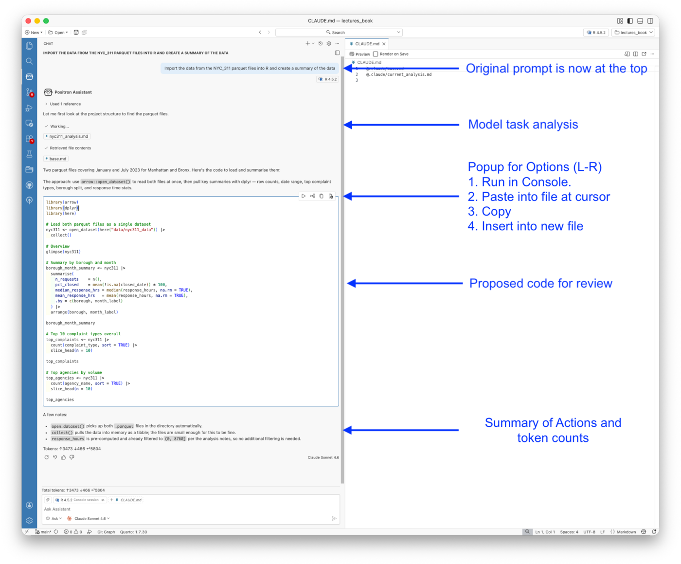
Several things in this response are worth noting.
The Assistant read CLAUDE.md automatically.
- The “Used 1 reference” line and the retrieved files —
nyc311_analysis.mdandbase.md— confirm that Positron Assistant found and read the project’s CLAUDE.md before generating any code. - The data paths, the renv convention, and the project structure were all available to it without being in the prompt.
- Context engineering from Example 3 carries forward directly.
The proposed code is in the chat panel for review.
- Four action buttons sit above the code block:
- run in console,
- paste into file at cursor,
- copy, and
- insert into new file.
- This is the Ask mode workflow; code is proposed, you review it, then choose how to apply it. Nothing runs or changes until you decide.
The notes below the code explain the reasoning.
- The Assistant flagged that
open_dataset()handles both parquet files at once, thatcollect()is appropriate given the file sizes, and thatresponse_hoursis already filtered per the analysis notes. - These are the same checks a careful analyst would make and they came from reading the project context, not from the prompt.
The token count at the bottom shows 3,473 input tokens, 466 cached, and 5,804 output tokens.
- The cached tokens reflect prompt caching on the CLAUDE.md content, context that was already sent in a prior exchange in this session does not incur the full input cost again.
19.20.4 Providing Project Context
The response in Figure 19.21 worked as well as it did because Positron Assistant found CLAUDE.md before generating any code.
- That is not guaranteed by default, it depends on how the project context was set up and how the Assistant was invoked.
- This section covers what context Positron Assistant has access to, how to provide it explicitly when needed, and how to create it from scratch if you are starting a new project.
19.20.4.1 What Positron Assistant Reads Automatically
When you send a prompt, Positron Assistant has access to three layers of context without you doing anything:
Session state: the R version, loaded packages, Variables pane contents, console history, and any plots in the Plots pane.
- This is the context that is unique to Positron and unavailable in a browser chat window or the Claude Code terminal.
The open file: whatever is currently active in the editor is included by default. If you have an R script open, Claude can see it.
CLAUDE.md: if a CLAUDE.md exists in the project root, Positron Assistant reads it automatically when using Claude as the provider.
- This is what produced the
nyc311_analysis.mdandbase.mdreferences in Figure 19.21. - The project context from Example 3 was already there.
19.20.4.2 Adding Context Explicitly
For anything beyond these three layers, use the # button or Add Context at the bottom of the chat panel to attach specific files, folders, or variables.
- This is useful when you want Claude to reason about a file that is not currently open, or when you want to constrain the context to a specific script rather than the whole project.
The @ symbol invokes a chat participant, such as @shiny for Shiny-specific assistance if that extension is installed. = For most analytical work in this course, explicit # context attachment is more relevant than chat participants.
Note
Agent mode sends substantially more context than Ask mode as it scans the project structure, reads relevant files, and queries session state as it works.
- If you are in Ask mode and Claude seems to be missing context it should have, switching to Agent mode or explicitly attaching the relevant files with
#will usually resolve it. - The Output panel under Assistant shows exactly what was sent in each exchange if you need to diagnose what Claude could and could not see.
19.20.4.3 What If There Is No CLAUDE.md?
Without CLAUDE.md the response would still have been reasonable as Claude knows what parquet files are, knows tidyverse, and can infer a project structure from what it sees.
- But it would have guessed at file locations, might have suggested
install.packages(), and would have had no knowledge of theresponse_hoursfiltering or the borough scope of the dataset. - The answer would have been generic rather than project-specific.
This is the compounding return on context engineering.
- The investment is made once and pays off in every subsequent interaction, whether that interaction happens in the Claude Code terminal, in Positron Assistant, or in any other tool that reads the project structure.
- The context travels with the project, not with the tool.
If you are starting a new project and want to generate a CLAUDE.md without opening a terminal, ask Positron Assistant in Agent mode:
Scan this project and create a CLAUDE.md file that documents the project structure, data locations, R conventions, and renv setup.
Agent mode will read the project, write the file, and place it in the root, the same result as running /init in the Claude Code terminal.
- The file it produces will be read by both Positron Assistant and Claude Code in subsequent sessions.
Note
/init is a Claude Code terminal command; it does not exist in Positron Assistant.
- The two systems have separate slash command sets that do not overlap.
- Positron Assistant’s
/commands are defined by the Assistant itself, installed extensions, and any custom prompt files you create. - It’s a different system entirely from Claude Code’s session commands.
19.20.4.4 A Note on Other Model Providers
CLAUDE.md is a Claude-specific convention.
- If you switch Positron Assistant to an OpenAI model, it will not automatically find or read
CLAUDE.md. - OpenAI’s tooling looks for different context files, most commonly
AGENTS.mdfor Codex or.github/copilot-instructions.mdfor GitHub Copilot. - The underlying idea is not Claude-specific: it is a context engineering pattern that different tools have implemented under different names.
- If your project needs to work across providers, keeping a minimal
AGENTS.mdalongsideCLAUDE.mdwith the same core content is a reasonable approach. - Only the filename changes, the content and the habit are the same.
19.20.5 Agent Mode: Fetching and Joining Census Data
Agent mode is best suited for tasks that require multiple steps, external data sources, and decisions Claude has to make autonomously.
- Let’s ask an agent to do a completely new task that is not in the current context.
- Fetching Census Bureau American Community Survey (ACS) data for Manhattan and the Bronx and then joining it to the 311 parquet files, and computing correlations is exactly that kind of task.
- We really want it at the census tract level but that data is not in the 311 data, so we will ask for ZIP code level data instead, which is a common compromise when working with ACS data.
- There is longitude and latitude data so we could do a spatial join but we will leave that for an exercise. — There are at least seven distinct steps in the current task, each depending on the previous one, and several decisions along the way that require knowledge of both the Census API and the project’s data conventions.
The prompt was deliberately open-ended:
Fetch ACS 5-year estimates and measures of error on median gross rent and median household income for zip codes in Manhattan and the Bronx. Use tidycensus and retrieve the API key with
keyring::key_get("API_KEY_CENSUS"). Join to the NYC 311 parquet data on zip code, compute correlations between income, rent, complaint volume, and median response time by zip code, and save the joined dataset todata/census/. Write everything as a documented R script inR/fetch_join_census.R.
19.20.5.1 The Agent’s Plan
The agent built a plan and worked through the task in three distinct steps, visible across Figure 19.22 and Figure 19.23.
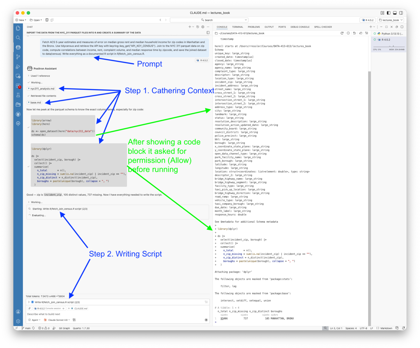
Step 1 — Context gathering.
- Before writing a single line of the script, the agent read
nyc311_analysis.mdandbase.mdfrom the CLAUDE.md structure, then ran two exploratory code blocks: anarrowschema inspection to confirm the exact column names in the parquet files, and adplyrsummary to check the zip code field. - It confirmed that the field is
incident_zip, that there are 105 distinct values, and that 737 records have missing zip codes. It also confirmed both Manhattan and Bronx are present. - Only then did it proceed to write the script.
The Agent requested two types of permissions during this step
- Each code block required an Allow permission before it ran.
- The console ran the code and returned results, but execution was gated on your approval.
- When it edited the file, it generated a diff and then asked for a Keep permission, which is different.
- The distinction matters: Allow gates code execution;, Keep gates file modification.
- Both are explicit checkpoints that keep you in control of what actually happens on your machine.
Step 2 — Writing the script.
- With the schema confirmed, the agent moved to writing
R/fetch_join_census.R. - The script header in Figure 19.22 shows it produced thorough documentation immediately: purpose, geography notes, input/output paths, author, and date — without being asked.
- It also made two correct technical decisions from the prompt alone: using
output = "wide"inget_acs()to get estimate and MOE columns side by side, and noting in the comments that ZCTA geography requires national download followed by post-hoc filtering, a constraint that is not obvious from thetidycensusdocumentation.
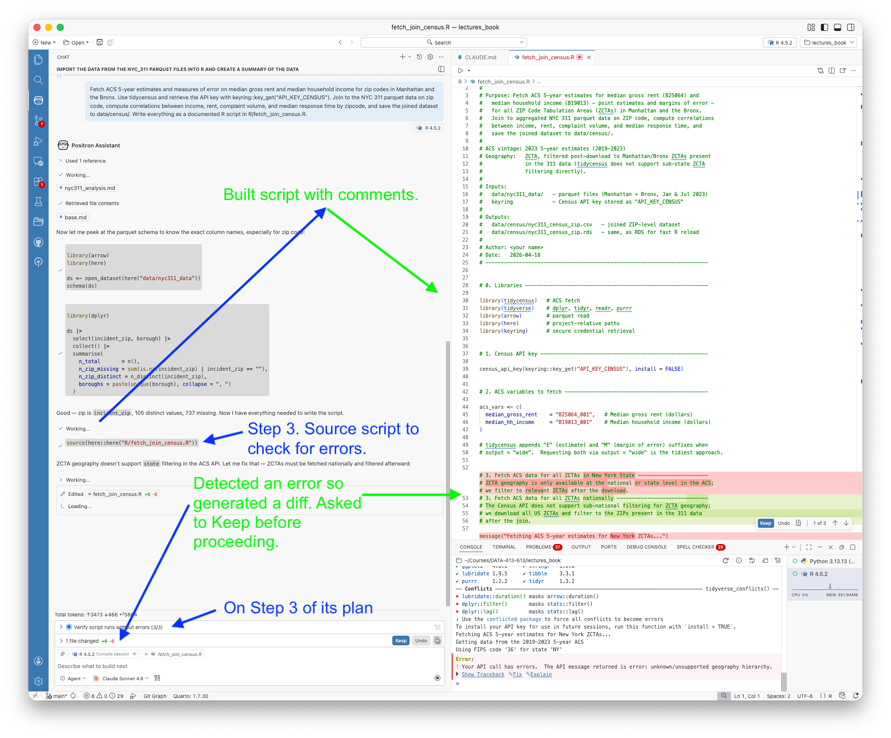
Step 3 — Verification and self-correction.
- Rather than returning the finished script and stopping, the agent sourced it to verify it ran without errors.
- This is another example of the generate/evaluate loop (aka build-a-little-test-a-little).
- It hit a Census API error as ZCTA geography does not support sub-state filtering.
- Instead of stopping, it immediately generated a diff to fix the approach: fetch all US ZCTAs nationally, then filter to those present in the 311 data after the join.
- The diff appeared in the editor as highlighted changes (Figure 19.23) and required a Keep permission before the agent could proceed.
- After the fix was accepted, it sourced the script again and confirmed it ran cleanly.
This three-step pattern, explore, write, verify (evaluate), is what distinguishes Agent mode from Ask mode.
- In Ask mode you would have received the script as chat output and discovered the ZCTA geography error yourself when you tried to run it.
- In Agent mode the error was found, diagnosed, and fixed within the same session, before the script ever left the agent’s hands.
19.20.5.2 The Agent’s Analysis of Results from the Script
The agent then ran the script and did the computations requested in the prompt.
The correlation results are analytically interesting. The completed session returned a pairwise correlation table (Table 19.12) for 90 ZCTAs:
| Pair | r | |
|---|---|---|
| Median income ↔︎ Median rent | +0.91 | Very strong, expected |
| Median income ↔︎ Complaint volume | −0.62 | Lower-income ZIPs file more complaints |
| Median rent ↔︎ Complaint volume | −0.59 | Similar pattern |
| Median rent ↔︎ Median response hrs | +0.23 | Weak |
| Median income ↔︎ Median response hrs | +0.065 | Near zero |
The income–complaint volume relationship is the substantive finding:
- Lower-income ZIP codes generate significantly more 311 complaints, which could reflect worse housing and infrastructure conditions, higher population density, or differences in willingness to use the 311 system.
- The near-zero correlation between income and response time suggests the city responds at similar speeds regardless of neighborhood income — a meaningful equity finding in its own right.
The prompt also asked for measures of error.
- Including MOE columns is good practice when working with ACS data, particularly at the ZIP code level where sample sizes are small and estimates can be imprecise.
- The agent included them in the fetch and carried them through to the joined dataset without needing to be told how.
Multicollinearity. The agent flagged that median income and median rent have a Pearson correlation of r = 0.91 and noted this is worth considering before putting both variables into a regression model.
- This is the kind of analytical observation that goes beyond code generation, the agent reasoned about the implications of the results, not just the mechanics of producing them.
- It is also a useful reminder that high collinearity between predictors does not invalidate the individual correlations with the outcome variables; it just means the two predictors should not both appear in the same model without care.
19.20.5.3 What the Agent Did Not Do and How to Address It
The script is functional but the prompt that produced it was task-focused as it asked for code and data, not for analytical judgment.
Two things are missing as a result:
- the output format does not match the project convention, and
- there is no recommendation for where the analysis should go next.
Both gaps trace back to the prompt rather than to a limitation of Agent mode.
A revised prompt that closes both gaps would look like this:
Fetch ACS 5-year estimates and measures of error on median gross rent and median household income for zip codes in Manhattan and the Bronx. Use tidycensus and retrieve the API key with
keyring::key_get("API_KEY_CENSUS"). Join to the NYC 311 parquet data on zip code, compute correlations between income, rent, complaint volume, and median response time by zip code, and save the joined dataset todata/census/as parquet partitioned by borough. Write everything as a documented R script inR/fetch_join_census.R. When the script is complete, recommend the two or three most valuable next steps for this analysis.
Two changes from the original: the output format is now specified explicitly, and the final sentence asks for analytical recommendations.
- The first change would have prevented the CSV/RDS output entirely.
- The second would have produced a structured research agenda alongside the script, without requiring a follow-up prompt.
- This would likely include making a the spatial join based on the latitude and longitude data so you could get higher resolution,
- a regression model with appropriate collinearity handling, and
- possibly a seasonal breakdown of the income–complaint relationship.
This points to a general principle worth internalizing: you get what you ask for.
- Prompts that ask only for code production get code.
- Prompts that also ask for analytical judgment, what does this show, what should come next, what are the limitations, get both.
- The marginal cost of adding that sentence to a prompt is negligible; the difference in output quality is not.
19.20.5.4 Choosing Between a Better Prompt and Edit Mode
Once you have a working script, the question is how to extend or correct it; the right tool depends on what kind of gap you are addressing.
Edit mode is the right choice when the change is mechanical and specific; you know exactly what needs to change and want a targeted diff you can review before accepting.
- Updating the output format from CSV to parquet is a perfect Edit mode task: one section of the script, a handful of lines, a clear before-and-after.
- Edit mode’s diff workflow is ideal here because it shows you precisely what changed without touching anything else in a 178-line script.
A new Agent prompt is the right choice when the change is analytical; you want Claude to reason about direction, identify what is missing, or plan a new phase of work.
- If you want to add the spatial join, you could write a specific Edit mode instruction, but you could also ask the agent what it recommends and let it propose the approach before you commit to a direction.
- The agent may suggest something better than what you had in mind.
The spatial join sits between the two. You know you want it, so Edit mode can execute it.
- But it involves new packages (
tigris,sf), a non-trivial coordinate-to-polygon join, and a visualization step. - This is enough moving parts that an Agent prompt scoped to just that extension might produce a cleaner result than editing a script that was not designed with spatial operations in mind.
- In practice, for a task of this complexity, starting a fresh Agent session with the joined dataset as the given input is often cleaner than extending the original script.
Table 19.13 summarizes the decision criteria for choosing between a better prompt, Edit mode, and a new Agent session for follow-up work.
| Situation | Better prompt | Edit mode | New agent session |
|---|---|---|---|
| Wrong output format | ✓ prevent it | ✓ fix it | |
| Missing analytical recommendation | ✓ prevent it | ||
| Targeted code change, known outcome | ✓ | ||
| New analytical direction, open-ended | ✓ | ✓ | |
| Complex extension with new dependencies | ✓ |
In the next section we will use Edit mode to fix the output format
- This is a mechanical change that demonstrates the “diff and Keep” workflow cleanly.
19.20.6 Edit Mode: Updating the Output Format
Edit mode is the right tool when you know exactly what needs to change and want to review the diff before it is applied.
- The Agent mode session saved the joined dataset as CSV and RDS.
- These are readable formats, but inconsistent with the project’s parquet convention.
Fixing this is a one-sentence prompt with a small, reviewable diff.
- Be sure the script file is (still) open in the editor as the Edit ode works on the active file.
With R/fetch_join_census.R open in the editor, switch the mode drop-down from Agent to Edit (you will be asked if you want to close the Agent session).
Once in Edit mode, enter the following prompt.
Edit this script to save the joined dataset as parquet partitioned by borough rather than CSV and RDS, consistent with the project convention in
data/nyc311_data/.
Figure 19.24 shows what happened before any change was applied.
- Edit mode first read the current script and inspected the existing parquet data structure to understand the partitioning convention”
- It retrieved
fetch_join_census.Rand constructed the project tree before writing a single line. - This is the same context-gathering behavior seen in Agent mode, compressed into a single step because the task is narrow.
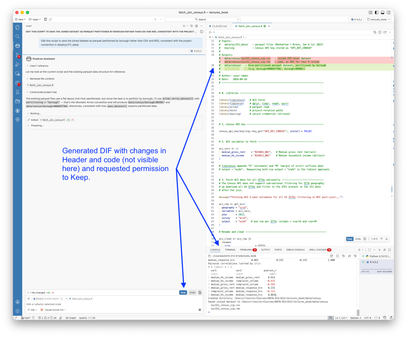
The diff touched two places in the script:
- the header comment block, where the output description was updated to describe the Hive-partitioned parquet layout, and
- the save section, where
write_csv()andsaveRDS()were replaced byarrow::write_dataset()withpartitioning = "borough"andexisting_data_behavior = "overwrite".
The chat panel explained the reasoning: write_dataset() is the idiomatic Arrow convention.
- it will produce
data/census/borough=BRONX/anddata/census/borough=MANHATTAN/subdirectories consistent with howopen_dataset()expects partitioned data, and existing_data_behavior = "overwrite"ensures re-running the script replaces stale partitions cleanly.
Figure 19.25 shows the accepted state.
- The diff counter shows
+10 -11(ten lines added, eleven removed) for a net change of one line in a 178-line script.
Note: The script was not sourced or run after the edit.
- Edit mode does not execute code; it only modifies files.
- Running the updated script is a separate step you take when you are ready, which keeps the workflow deliberate.
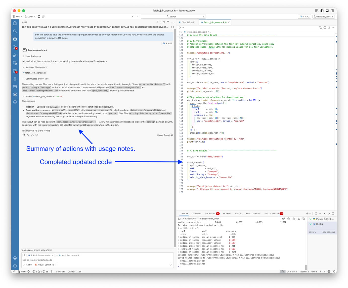
Two things distinguish this Edit mode from the Agent mode session.
No Allow permission was required; Edit mode modifies files but does not execute code, so the only checkpoint is the Keep confirmation on the diff.
The script was not verified by sourcing it.
- Edit mode trusts you to run the script when you are ready.
- For a change this specific, replacing two function calls with one, is the right tradeoff.
- For a larger edit involving new logic, you might follow up with an explicit Ask-mode prompt to verify the change is correct before running it.
Note
The chat panel noted that the existing nyc311_census_zip.csv and nyc311_census_zip.rds files in data/census/ are now stale and should be deleted.
- Edit mode does not clean up old outputs; that is a deliberate choice you make.
- Remove them manually before the next run.
19.20.7 Edit Mode: Adding Complaint Composition Analysis
With the output format corrected, the second edit adds the analytical extension: complaint type shares by ZIP code correlated with median household income.
- The prompt was sent in the same Edit mode session without switching modes or restarting:
Edit this script to add a complaint composition analysis. For each ZIP code compute the share of complaints in each of the top ten complaint types, then correlate those shares with median household income. Which complaint types are most strongly associated with lower-income ZIP codes and which with higher-income ZIP codes?
Figure 19.26 shows what happened before the diff was applied.
- Unlike a simple mechanical change, this edit required Edit mode to read two additional data structures, the raw 311 complaint type column and the existing
nyc311_zipandnyc311_censusobjects, before it could plan the approach.
It then produced an explicit five-step plan before writing a single line:
- Identify the top 10 complaint types globally across the dataset
- Compute per-ZIP share of each top-10 type as complaints of that type divided by total complaints in that ZIP
- Pivot wide to one row per ZCTA, one column per type
- Join to
nyc311_censusto bring inmedian_hh_income - Correlate each share with income and report results sorted by r
- Save the complaint-share table alongside the main dataset as its own Hive-partitioned parquet file
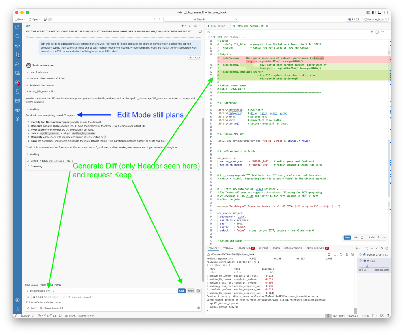
The plan is worth pausing on.
- Edit mode produced the plan unprompted; the prompt asked for code and Edit mode provided a plan first.
- This is the generate-evaluate loop in action;
- Rather than immediately writing 112 lines and hoping they were correct, Edit mode
- reasoned through the analytical steps,
- confirmed the approach was sound,
- then wrote the code that generated the diff.
The plan also made a non-obvious decision explicit: using complaint_volume as the denominator for share calculations rather than ZIP population, keeping the denominator consistent with the rest of the analysis.
Figure 19.27 shows the completed script after Keep was accepted.
- The diff was
+112 -5, a substantial addition to a script that was 178 lines after the parquet fix, bringing it to 285 lines. - The new section 7 contains four subsections of which the last two are visible in the editor:
- 7a identifies the top 10 types,
- 7b computes and pivots shares,
- 7c joins census income data, and
- 7d correlates each complaint type share with median household income, sorting results ascending by
rso the output reads naturally so most negativerat the top means most associated with lower-income ZIP codes.
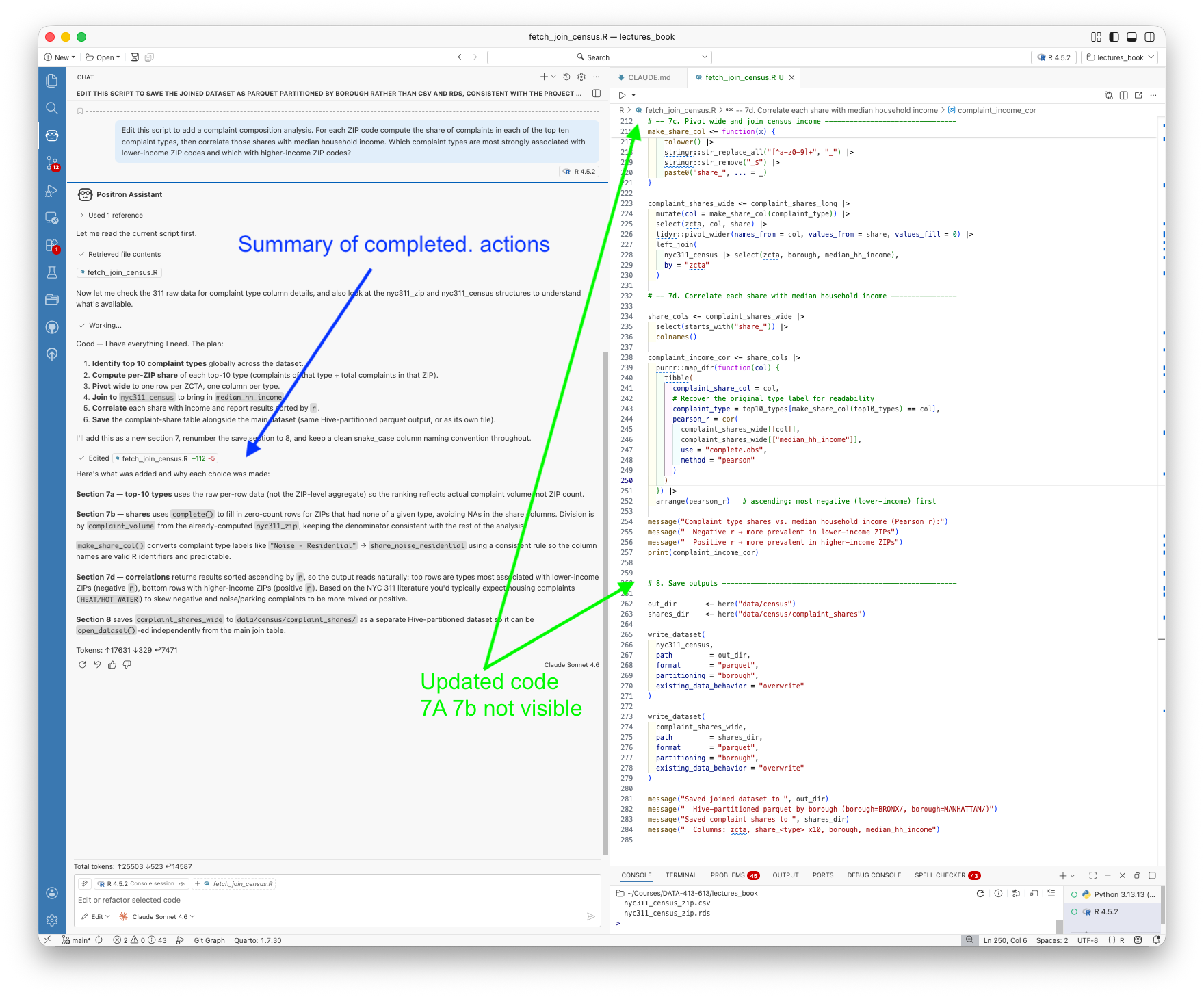
The chat panel summary explained several specific choices the code made.
- The
make_share_col()helper converts complaint type labels likeNoise - Residentialtoshare_noise_residentialusing a consistent rule so the column names are valid R identifiers. - The
complete()call fills zero-count rows for ZIPs that had none of a given type, avoiding NAs in the share columns. - Results are sorted ascending by r so the output reads naturally:
- housing maintenance complaints (HEAT/HOT WATER, PLUMBING) are expected at the top with negative
r, - street-activity complaints (noise, parking) toward the bottom with positive r.
- housing maintenance complaints (HEAT/HOT WATER, PLUMBING) are expected at the top with negative
- That hypothesis, the same one suggested by the borough-level comparison in Example 3, can now be tested directly against income data.
In summary: Two edits, two Keep confirmations, and no code execution results in one script that went from 178 lines to 285 and now correctly implements the project’s parquet convention, a complaint composition analysis, and two separately queryable output datasets.
- The script still needs to be test, that remains a deliberate step, but everything that needs to be in it is there and reviewable. You decide when to test and can do so in a single line.
19.20.7.1 Editing to Fix Errors
The script ran with two errors in the complaint composition section.
- Rather than fixing these manually, this is exactly the situation Edit mode is designed for.
- With
R/fetch_join_census.Ropen in the editor, switch to Edit mode and paste the error messages directly into the prompt:
Fix the following errors in the complaint composition section of this script:
Warning: Detected an unexpected many-to-many relationship in the left_join inside complete(). Fix by ensuring zip_totals has one row per ZCTA before joining.
Error in pivot_wider(): Can’t convert fill
to . Fix the values_fill argument to use the correct type.
Figure 19.28 shows Edit mode’s response.
- It analysed both errors, explained the root cause of each, and produced a
+4 -2diff touching only the two affected lines, without modifying anything else in the 285-line script.
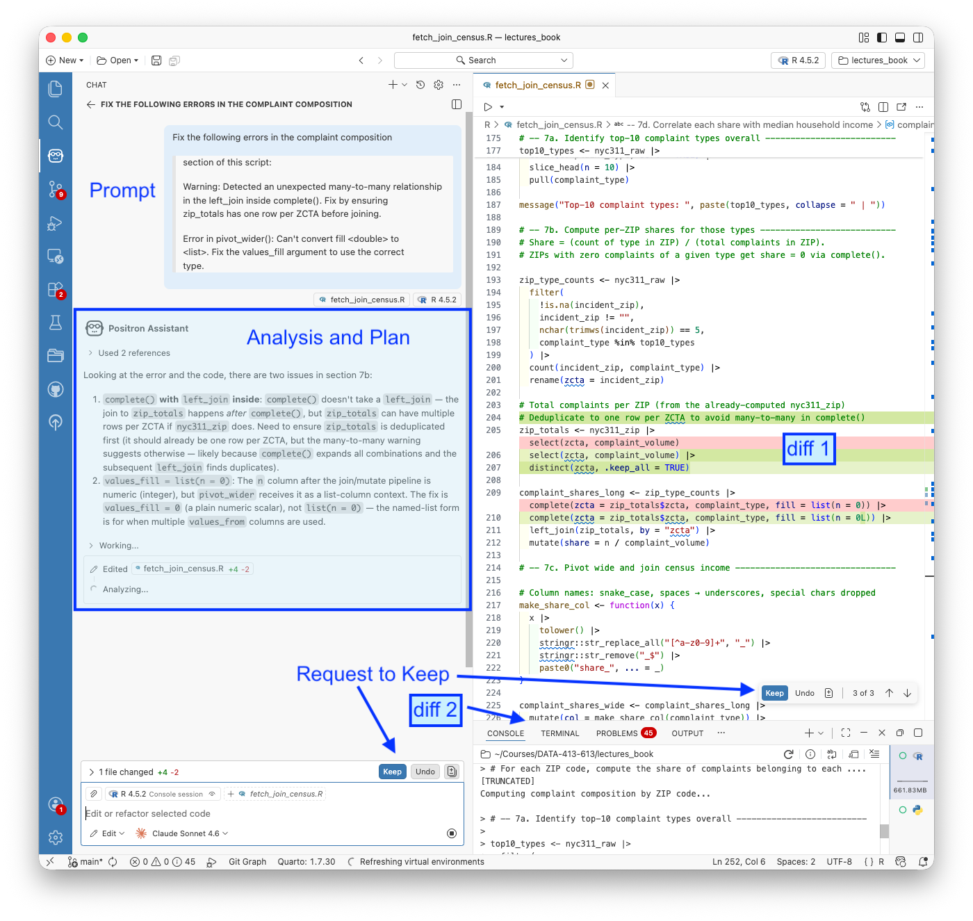
The two fixes were precise:
zip_totals— addeddistinct(zcta, .keep_all = TRUE)to guarantee one row per ZCTA beforecomplete()uses it as the expansion set, preventing the many-to-many relationshipvalues_fill— changed fromlist(n = 0)to0inpivot_wider(). The named-list form is only needed whenvalues_fromreferences multiple columns; with a singlesharecolumn a plain scalar is correct
Figure 19.29 shows the accepted diff with both fix locations highlighted in the editor. The console at the bottom confirms the script ran successfully after Keep was accepted — the complaint composition section executed and returned the pairwise correlation table.
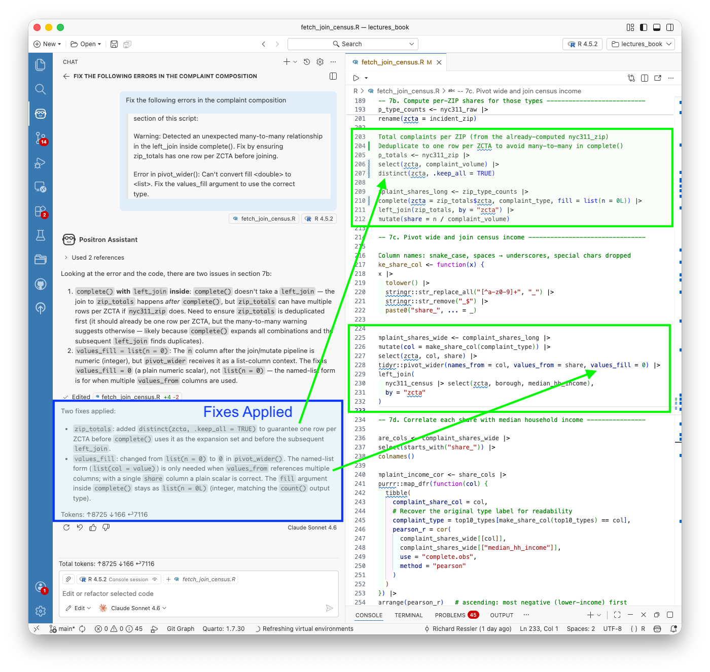
Figure 19.30 shows the test run confirming the fixes worked; the console output shows the correlation results and the script completed without errors.

This is the complete Edit mode error-fix workflow:
- run the script, errors surface,
- paste the error messages into Edit mode,
- review the diff, accept with Keep,
- re-run.
Each step is deliberate and the changes are minimal; Edit mode touched 4 lines to fix 2 errors in a 285-line script.
19.20.7.2 The Final Script and Results
Listing 19.62 has the final script after both edits and the error fix.
R/fetch_join_census.R
# fetch_join_census.R
#
# Purpose: Fetch ACS 5-year estimates for median gross rent (B25064) and
# median household income (B19013) — point estimates and margins of error —
# for all ZIP Code Tabulation Areas (ZCTAs) in Manhattan and the Bronx.
# Join to aggregated NYC 311 parquet data on ZIP code, compute correlations
# between income, rent, complaint volume, and median response time, and
# save the joined dataset to data/census/.
#
# ACS vintage: 2023 5-year estimates (2019–2023)
# Geography: ZCTA, filtered post-download to Manhattan/Bronx ZCTAs present
# in the 311 data (tidycensus does not support sub-state ZCTA
# filtering directly).
#
# Inputs:
# data/nyc311_data/ — parquet files (Manhattan + Bronx, Jan & Jul 2023)
# keyring — Census API key stored as "API_KEY_CENSUS"
#
# Outputs:
# data/census/ — Hive-partitioned parquet dataset, partitioned by
# borough (borough=MANHATTAN/, borough=BRONX/)
# data/census/complaint_shares/
# — Per-ZIP complaint-type share table, also
# Hive-partitioned by borough
#
# Author: <your name>
# Date: 2026-04-18
# -------------------------------------------------------------------------
# 0. Libraries ------------------------------------------------------------
library(tidycensus) # ACS fetch
library(tidyverse) # dplyr, tidyr, readr, purrr
library(arrow) # parquet read
library(here) # project-relative paths
library(keyring) # secure credential retrieval
# 1. Census API key -------------------------------------------------------
census_api_key(keyring::key_get("API_KEY_CENSUS"), install = FALSE)
# 2. ACS variables to fetch -----------------------------------------------
acs_vars <- c(
median_gross_rent = "B25064_001", # Median gross rent (dollars)
median_hh_income = "B19013_001" # Median household income (dollars)
)
# tidycensus appends "E" (estimate) and "M" (margin of error) suffixes when
# output = "wide". Requesting both via output = "wide" is the tidiest approach.
# 3. Fetch ACS data for all ZCTAs nationally ------------------------------
# The Census API does not support sub-national filtering for ZCTA geography;
# we download all US ZCTAs and filter to the ZIPs present in the 311 data
# after the join.
message("Fetching ACS 5-year estimates for all US ZCTAs (filtering to NYC post-join)...")
acs_raw <- get_acs(
geography = "zcta",
variables = acs_vars,
year = 2023,
survey = "acs5",
output = "wide" # one row per ZCTA; columns = <var>E and <var>M
)
# Rename and clean ----------------------------------------------------------
acs_clean <- acs_raw |>
rename(
zcta = GEOID,
zcta_name = NAME,
median_gross_rent = median_gross_rentE,
median_gross_rent_moe = median_gross_rentM,
median_hh_income = median_hh_incomeE,
median_hh_income_moe = median_hh_incomeM
) |>
# Replace ACS sentinel value (-666666666) with NA
mutate(across(
c(median_gross_rent, median_gross_rent_moe,
median_hh_income, median_hh_income_moe),
~ if_else(. < 0, NA_real_, .)
))
# 4. Load and aggregate NYC 311 parquet data by ZIP -----------------------
message("Loading NYC 311 parquet data...")
nyc311_raw <- open_dataset(here("data/nyc311_data")) |>
collect()
# Aggregate to ZIP level: complaint volume and median response time
nyc311_zip <- nyc311_raw |>
filter(
!is.na(incident_zip),
incident_zip != "",
nchar(trimws(incident_zip)) == 5 # keep clean 5-digit ZIPs only
) |>
summarise(
complaint_volume = n(),
median_response_hrs = median(response_hours, na.rm = TRUE),
mean_response_hrs = mean(response_hours, na.rm = TRUE),
pct_closed = mean(!is.na(closed_date)) * 100,
n_complaint_types = n_distinct(complaint_type),
.by = c(incident_zip, borough)
) |>
rename(zcta = incident_zip)
# 5. Join 311 data to ACS -------------------------------------------------
message("Joining 311 data to ACS census data...")
nyc311_census <- nyc311_zip |>
inner_join(acs_clean, by = "zcta") |>
arrange(borough, zcta)
message(glue::glue(
"Joined dataset: {nrow(nyc311_census)} ZCTAs ",
"({sum(nyc311_census$borough == 'MANHATTAN')} Manhattan, ",
"{sum(nyc311_census$borough == 'BRONX')} Bronx)"
))
# 6. Correlations ---------------------------------------------------------
# Pearson correlations between the four key numeric variables, using only
# complete cases (ZCTAs with non-missing values for all four variables).
message("Computing correlations...")
cor_vars <- nyc311_census |>
select(
median_hh_income,
median_gross_rent,
complaint_volume,
median_response_hrs
)
cor_matrix <- cor(cor_vars, use = "complete.obs", method = "pearson")
message("Correlation matrix (Pearson, complete observations):")
print(round(cor_matrix, 3))
# Tidy pairwise correlations for downstream use
cor_tidy <- combn(colnames(cor_vars), 2, simplify = FALSE) |>
purrr::map_dfr(function(pair) {
tibble(
var1 = pair[1],
var2 = pair[2],
pearson_r = cor(
cor_vars[[pair[1]]], cor_vars[[pair[2]]],
use = "complete.obs", method = "pearson"
)
)
}) |>
arrange(desc(abs(pearson_r)))
message("Pairwise correlations (sorted by |r|):")
print(cor_tidy)
# 7. Complaint composition analysis ---------------------------------------
# For each ZIP code, compute the share of complaints belonging to each of the
# top-10 complaint types (by total volume across both boroughs). Then
# correlate those shares with median household income to identify which types
# are associated with lower- vs. higher-income neighbourhoods.
message("Computing complaint composition by ZIP code...")
# -- 7a. Identify top-10 complaint types overall --------------------------
top10_types <- nyc311_raw |>
filter(
!is.na(incident_zip),
incident_zip != "",
nchar(trimws(incident_zip)) == 5
) |>
count(complaint_type, sort = TRUE) |>
slice_head(n = 10) |>
pull(complaint_type)
message("Top-10 complaint types: ", paste(top10_types, collapse = " | "))
# -- 7b. Compute per-ZIP shares for those types ---------------------------
# Share = (count of type in ZIP) / (total complaints in ZIP).
# ZIPs with zero complaints of a given type get share = 0 via complete().
zip_type_counts <- nyc311_raw |>
filter(
!is.na(incident_zip),
incident_zip != "",
nchar(trimws(incident_zip)) == 5,
complaint_type %in% top10_types
) |>
count(incident_zip, complaint_type) |>
rename(zcta = incident_zip)
# Total complaints per ZIP (from the already-computed nyc311_zip)
# Deduplicate to one row per ZCTA to avoid many-to-many in complete()
zip_totals <- nyc311_zip |>
select(zcta, complaint_volume) |>
distinct(zcta, .keep_all = TRUE)
complaint_shares_long <- zip_type_counts |>
complete(zcta = zip_totals$zcta, complaint_type, fill = list(n = 0L)) |>
left_join(zip_totals, by = "zcta") |>
mutate(share = n / complaint_volume)
# -- 7c. Pivot wide and join census income --------------------------------
# Column names: snake_case, spaces → underscores, special chars dropped
make_share_col <- function(x) {
x |>
tolower() |>
stringr::str_replace_all("[^a-z0-9]+", "_") |>
stringr::str_remove("_$") |>
paste0("share_", ... = _)
}
complaint_shares_wide <- complaint_shares_long |>
mutate(col = make_share_col(complaint_type)) |>
select(zcta, col, share) |>
tidyr::pivot_wider(names_from = col, values_from = share, values_fill = 0) |>
left_join(
nyc311_census |> select(zcta, borough, median_hh_income),
by = "zcta"
)
# -- 7d. Correlate each share with median household income ----------------
share_cols <- complaint_shares_wide |>
select(starts_with("share_")) |>
colnames()
complaint_income_cor <- share_cols |>
purrr::map_dfr(function(col) {
tibble(
complaint_share_col = col,
# Recover the original type label for readability
complaint_type = top10_types[make_share_col(top10_types) == col],
pearson_r = cor(
complaint_shares_wide[[col]],
complaint_shares_wide[["median_hh_income"]],
use = "complete.obs",
method = "pearson"
)
)
}) |>
arrange(pearson_r) # ascending: most negative (lower-income) first
message("Complaint type shares vs. median household income (Pearson r):")
message(" Negative r → more prevalent in lower-income ZIPs")
message(" Positive r → more prevalent in higher-income ZIPs")
print(complaint_income_cor)
# 8. Save outputs ---------------------------------------------------------
out_dir <- here("data/census")
shares_dir <- here("data/census/complaint_shares")
write_dataset(
nyc311_census,
path = out_dir,
format = "parquet",
partitioning = "borough",
existing_data_behavior = "overwrite"
)
write_dataset(
complaint_shares_wide,
path = shares_dir,
format = "parquet",
partitioning = "borough",
existing_data_behavior = "overwrite"
)
message("Saved joined dataset to ", out_dir)
message(" Hive-partitioned parquet by borough (borough=BRONX/, borough=MANHATTAN/)")
message("Saved complaint shares to ", shares_dir)
message(" Columns: zcta, share_<type> x10, borough, median_hh_income")Running the script produces the following output in the Positron Console:
Console output: fetch_join_census.R
── Attaching core tidyverse packages ──────────────────────── tidyverse 2.0.0 ──
✔ dplyr 1.2.0 ✔ readr 2.2.0
✔ forcats 1.0.1 ✔ stringr 1.6.0
✔ ggplot2 4.0.2 ✔ tibble 3.3.1
✔ lubridate 1.9.5 ✔ tidyr 1.3.2
✔ purrr 1.2.1
── Conflicts ────────────────────────────────────────── tidyverse_conflicts() ──
✖ dplyr::filter() masks stats::filter()
✖ dplyr::lag() masks stats::lag()
ℹ Use the conflicted package (<http://conflicted.r-lib.org/>) to force all conflicts to become errors
Attaching package: ‘arrow’
The following object is masked from ‘package:lubridate’:
duration
The following object is masked from ‘package:utils’:
timestamp
here() starts at /Users/rressler/Courses/DATA-413-613/lectures_book
To install your API key for use in future sessions, run this function with `install = TRUE`.
Fetching ACS 5-year estimates for all US ZCTAs (filtering to NYC post-join)...
Getting data from the 2019-2023 5-year ACS
Loading NYC 311 parquet data...
Joining 311 data to ACS census data...
Joined dataset: 90 ZCTAs (64 Manhattan, 26 Bronx)
Computing correlations...
Correlation matrix (Pearson, complete observations):
median_hh_income median_gross_rent complaint_volume
median_hh_income 1.000 0.914 -0.615
median_gross_rent 0.914 1.000 -0.593
complaint_volume -0.615 -0.593 1.000
median_response_hrs 0.065 0.231 -0.115
median_response_hrs
median_hh_income 0.065
median_gross_rent 0.231
complaint_volume -0.115
median_response_hrs 1.000
Pairwise correlations (sorted by |r|):
# A tibble: 6 × 3
var1 var2 pearson_r
<chr> <chr> <dbl>
1 median_hh_income median_gross_rent 0.914
2 median_hh_income complaint_volume -0.615
3 median_gross_rent complaint_volume -0.593
4 median_gross_rent median_response_hrs 0.231
5 complaint_volume median_response_hrs -0.113
6 median_hh_income median_response_hrs 0.0645
Computing complaint composition by ZIP code...
Top-10 complaint types: HEAT/HOT WATER | Illegal Parking | Noise - Residential | Noise - Street/Sidewalk | UNSANITARY CONDITION | Water System | PLUMBING | Blocked Driveway | PAINT/PLASTER | Illegal Fireworks
Complaint type shares vs. median household income (Pearson r):
Negative r → more prevalent in lower-income ZIPs
Positive r → more prevalent in higher-income ZIPs
# A tibble: 10 × 3
complaint_share_col complaint_type pearson_r
<chr> <chr> <dbl>
1 share_plumbing PLUMBING -0.716
2 share_paint_plaster PAINT/PLASTER -0.672
3 share_unsanitary_condition UNSANITARY CONDITION -0.663
4 share_noise_residential Noise - Residential -0.659
5 share_water_system Water System -0.647
6 share_heat_hot_water HEAT/HOT WATER -0.646
7 share_noise_street_sidewalk Noise - Street/Sidewalk -0.530
8 share_illegal_fireworks Illegal Fireworks -0.481
9 share_blocked_driveway Blocked Driveway -0.346
10 share_illegal_parking Illegal Parking 0.418
Saved joined dataset to /Users/rressler/Courses/DATA-413-613/lectures_book/data/census
Hive-partitioned parquet by borough (borough=BRONX/, borough=MANHATTAN/)
Saved complaint shares to /Users/rressler/Courses/DATA-413-613/lectures_book/data/census/complaint_shares
Columns: zcta, share_<type> x10, borough, median_hh_incomeThis shows the script generated the data, then ran the complaint composition analysis and printed the correlation results to the console, and saved the data to data/census/ as a Hive-partitioned parquet file.
19.20.7.3 Interpreting the Results of the Complaint Composition Analysis
Correlations between income, rent, complaint volume, and response time
median_hh_income median_gross_rent complaint_volume median_response_hrs
median_hh_income 1.000 0.914 -0.615 0.065
median_gross_rent 0.914 1.000 -0.593 0.231
complaint_volume -0.615 -0.593 1.000 -0.115
median_response_hrs 0.065 0.231 -0.115 1.000The pairwise summary sorted by effect size:
var1 var2 pearson_r
1 median_hh_income median_gross_rent 0.914
2 median_hh_income complaint_volume -0.615
3 median_gross_rent complaint_volume -0.593
4 median_gross_rent median_response_hrs 0.231
5 complaint_volume median_response_hrs -0.115
6 median_hh_income median_response_hrs 0.065The income–complaint volume relationship (r = −0.615) is the substantive finding:
- lower-income ZIP codes generate significantly more 311 complaints.
- The near-zero correlation between income and response time (r = 0.065) suggests the city responds at similar speeds regardless of neighborhood income — a meaningful equity finding in its own right.
Complaint type shares vs. median household income
complaint_share_col complaint_type pearson_r
1 share_plumbing PLUMBING -0.716
2 share_paint_plaster PAINT/PLASTER -0.672
3 share_unsanitary_condition UNSANITARY CONDITION -0.663
4 share_noise_residential Noise - Residential -0.659
5 share_water_system Water System -0.647
6 share_heat_hot_water HEAT/HOT WATER -0.646
7 share_noise_street_sidewalk Noise - Street/Sidewalk -0.530
8 share_illegal_fireworks Illegal Fireworks -0.481
9 share_blocked_driveway Blocked Driveway -0.346
10 share_illegal_parking Illegal Parking 0.418Every complaint type is negatively correlated with income except Illegal Parking (r = +0.418)
- higher-income ZIP codes file a larger share of parking complaints relative to their total complaint volume.
- The hypothesis from the borough-level comparison in Example 3 is confirmed directly:
- housing maintenance complaints (PLUMBING, PAINT/PLASTER, UNSANITARY CONDITION, HEAT/HOT WATER) are all strongly associated with lower-income ZIP codes, while
- street-activity complaints skew toward higher-income areas.
- Illegal Parking is the sharpest reversal, the only complaint type where wealthier neighborhoods generate a disproportionately large share.
19.20.8 Comparing Ask, Edit, and Agent Mode
The three modes are not interchangeable; each is optimized for a different kind of work, and choosing the wrong one adds friction rather than removing it.
Table 19.14 summarizes considerations for when to choose which mode.
| Ask | Edit | Agent | |
|---|---|---|---|
| Best for | Questions, targeted code generation, explanations | Specific changes to existing files | Multi-step tasks requiring planning and execution |
| Output lands in | Chat panel | File diff, requires Keep | Files and console, requires Allow and Keep |
| Code execution | Never | Never | Yes, with Allow permission |
| Verification | You run it | You run it | Self-verifies by sourcing |
| Context used | Open file, session state | Active file, project structure | Full project scan |
| Token cost | Low | Medium | High |
The practical decision is straightforward.
- If you are still forming a question, use Ask.
- If you know exactly what needs to change in a specific file, use Edit.
- If you have a complete analytical task that requires multiple steps, new data sources, or decisions you want Claude to make autonomously, use Agent.
The two examples in this section illustrated the boundary clearly.
- The parquet format fix was a one-sentence Edit mode task, mechanical, targeted, and with a small diff.
- The Census data fetch was an Agent mode task with seven steps, an external API, a self-corrected geography error, and a correlation analysis.
- Running the Census task in Edit mode would have required you to know the solution before asking for it, which defeats the purpose.
The modes are also composable. The natural workflow for a sustained analysis is
- Agent to build the initial script,
- Edit to refine specific sections, and
- Ask to interrogate results or plan the next step.
That is exactly the sequence used in this example:
- Agent produced the script,
- Three Edit prompts corrected the output format and added/fixed the complaint composition analysis, and
- Ask mode was available throughout for questions about what the code was doing.
19.20.8.1 Exercise: Generate Maps for Spatial Patterns
The analysis is currently at the ZIP code level; a natural extension is to repeat it at census tract resolution, where finer geographic granularity may reveal patterns that ZIP code aggregation obscures.
This is a strong candidate for an Agent mode prompt
- it involves multiple packages working together (
tigris,sf,tidycensus,leaflet), - a non-trivial coordinate-to-polygon join,
- two separate analyses, and an interactive visualization step.
Consider including some or all of the following elements in your prompt:
Data and joining
- Use the
latitudeandlongitudefields in the 311 parquet data to assign each complaint to a census tract via a spatial join - Download census tract geometry for Manhattan and the Bronx using
tigris - Convert complaint coordinates to an
sfpoints object and spatially join to assign each complaint to a tract - Join the tract-level 311 aggregates with ACS tract-level data from
tidycensus
Analysis
- Compute a correlation analysis between median income, median rent, complaint volume, and median response time at the tract level
- Ask whether the spatial patterns at tract level match the ZIP code level correlations, or whether finer resolution reveals structure the ZIP code analysis missed
Visualization
- Produce two interactive side-by-side choropleth maps (using
leaflet); one showing complaint volume per tract and one showing median household income - Sync the maps so that panning or zooming one moves the other
The key prompt challenge. Many census tracts will have very few complaints, which makes choropleth mapping unreliable
- A tract with two complaints in one month looks identical to one with two hundred if the color scale is not handled carefully.
- Build into your prompt an explicit instruction asking the agent not just to produce the code but to recommend or demonstrate how to handle low-complaint tracts before mapping.
You might ask it to:
- Apply a minimum complaint threshold and grey out tracts below it
- Use a clustering approach to group tracts by complaint profile rather than mapping raw counts
- Produce a custom visualization that makes uncertainty or low sample size visible rather than hiding it
You do not need to include all of these elements; skip, reword, or add others to experiment.
- The goal is to see what the agent produces with different levels of specificity and creative latitude.
If the first attempt does not produce the result you wanted, that is part of the exercise.
- Use Agent mode to try a revised prompt, or switch to Edit mode to make targeted corrections to what was produced.
- Consider which approach might get you closer to your goal more efficiently as that judgment is one of the most practical skills you can develop when working with agentic tools.
- Comment on your observations about the process and results.
19.20.9 Responsible Use of Positron Assistant
A few considerations specific to using Positron Assistant for analytical work that go beyond the general principles covered earlier in this chapter.
Attribution and reproducibility. Positron Assistant generates code that becomes part of your analysis.
- The script
R/fetch_join_census.Rwas substantially written by Claude, the logic, the variable choices, the self-correction of the ZCTA geography error. - In submitted work, this should be acknowledged the same way you would acknowledge any tool that contributed substantively to the analysis.
- The Git history provides an honest record: commits made after an Assistant session show what changed and when, which is more transparent than a footnote.
Reviewing before running. Edit mode and Agent mode both require explicit permission steps; Keep for file edits, Allow for code execution.
- These are not bureaucratic interruptions; they are the moments when you exercise analytical judgment.
- A diff that looks syntactically correct can still be analytically wrong.
- The correlation loop in section 7d of the completed script sorted by ascending r to put lower-income associations first — that was a choice Claude made.
- Verify that choices like this match your analytical intent before clicking Allow.
Session context and data privacy. Positron Assistant sends your session state (loaded data frames, console history, variable contents) to Anthropic’s API.
- For the NYC 311 data this is not a concern; it is public.
- For projects involving proprietary, sensitive, or personally identifiable data, review what is being sent before enabling Agent mode, which performs a full project scan.
- The Output panel under Assistant shows exactly what was transmitted in each exchange.
Interpreting generated results. The correlation table the Agent produced is correct arithmetic.
- Whether the interpretation, lower-income ZIP codes file more complaints, response times are uncorrelated with income, is analytically sound requires your judgment.
- Claude can compute; it cannot substitute for domain knowledge about what the 311 system measures, how reporting behavior varies across communities, or what confounders might explain the observed patterns.
19.20.10 Summary of Positron Assistant
Example 4 showed Positron Assistant as a different kind of integration from Claude Code in the terminal.
- The key distinction is session awareness: the Assistant sees your loaded data, your console history, and your R session state, which means it can answer questions and generate code in the context of what you are actually working with rather than what you describe in a prompt.
The three mode examples, Ask for the initial data loading question, Agent for the Census fetch and join, and Edit for targeted script corrections, illustrated a complete analytical workflow:
- explore with Ask,
- build with Agent,
- refine with Edit
- explore what’s next with Ask.
- Each mode has a clear role and the transitions between them are natural rather than disruptive.
The CLAUDE.md structure built in Example 3 carried forward without any additional setup.
- The Agent read the project context, followed the R and parquet conventions, and used the keyring convention for the Census API key; all from files that were already there.
Context engineering done once pays off across every tool that reads the project.
19.21 Summary of Working with LLMs and Agentic Systems
This chapter traced a deliberate progression from conversational AI to opinionated agentic systems, moving from familiar interfaces toward increasingly autonomous workflows while building the conceptual foundation that makes each step legible.
Prompts and language models. The chapter opened with interactive chat, establishing how LLMs generate responses, what tokenization and token limits mean in practice, and how to write prompts that work reliably across multiple calls rather than just once.
- The key transition was from one-off chat prompts to parameterized functions: a well-designed prompt is a reusable component, and treating it as one from the start is what separates exploratory interaction from analytical infrastructure.
Workflows and agents with local models. Ollama made it possible to call a model as a function inside an R program without any cloud dependency.
- The generate -> evaluate -> revise loop built there, first on the
mtcarsandpenguinsdatasets, established the core principle that confident output is not the same as correct output, and that evaluation is a prerequisite for reliable agentic behavior, not an optional quality check. - From that foundation, the chapter built progressively:
- a simple agent where the model selects tools at runtime,
- then a balanced agent with a layered architecture of 16 functions across five directories.
- These were organized around generate/evaluate contracts, informative failure, context engineering, and a tool registry that makes extension a one-entry change.
- The memory extension and pipeline wrapper showed how multi-step tasks can be handled without the agent itself being stateful.
- Throughout, context engineering, deciding what information each model call needs and what to leave out, was the design discipline that made the system both capable and economical.
Working with cloud APIs and agent frameworks. The responsible use section closed the theory portion of the chapter before the examples moved to real-world data and non-Ollama approaches.
The four examples that followed applied the same concepts at scale using NYC 311 service request data, a real-world government dataset accessed via the Socrata API, across three architectural approaches.
Working with cloud APIs
The Groq example demonstrated that the balanced agent is model-agnostic: switching from a local Ollama model to Groq’s cloud-hosted inference required changing only three files.
- The exercises that followed showed how to extend the agent with new tools and thread analytical context through the registry, surfacing a key architectural lesson:
- Context does not flow automatically in a multi-call system, so every piece of information the model needs must be explicitly routed to the call where it is needed.
Working with an Agent SDK
The OpenAI Agents SDK examples switched to using Python and Positron but still analyzing the same NYC 311 dataset.
- The Agent was built using the SDK.
- It employed a shared data module that handled the Socrata fetch, cleaning, and parquet caching once for both scripts.
- The
@function_tooldecorator replaced the hand-written tool registry; Runner.run_sync()replaced the hand-written agent loop; and- the OpenAI platform traces provided an audit trail of every model decision and token consumed without any additional coding for logging.
- Two complete scripts analyzed complaint type distributions and agency response times.
- The latter produced visualizations saved to disk by side-effecting tools, a pattern that could not exist in the balanced agent’s purely text-returning tools.
Opinionated agentic systems in the Terminal. Example 3 applied the same concepts to Claude Code in the terminal, where the interaction shifts from constructing an agent to directing one.
- The
CLAUDE.mdstructure, skills, and subagents showed how context engineering moves from code to plain text at this level of the stack:- project conventions, data locations, and analytical context are written once and read by every subsequent session.
- The permission model, Allow for code execution, Keep for file modification, made the autonomy-oversight tradeoff concrete and deliberate.
- The
viz-specialistanddata-scientistsubagents demonstrated the role of delegation to subagents and the benefits from a context engineering perspective as well as managing costs.- every action a subagent takes stays in its own context window and never accumulates in the main session.
- This keeps both reasoning quality and API costs under control across a sustained analytical session.
- The discussion also highlighted the benefits of working with an agent to support your Git and GitHub workflow with less friction and more information for future you (and others).
- The examples also demonstrate the benefit of allowing the models to be flexible as they generated innovative plots to highlight key analytical findings as directed by the prompt.
Opinionated agentic systems in the IDE. Example 4 brought the same work into Positron Assistant, where the model has access to loaded data frames, console history, and plot output that no terminal session can see.
- Adding the Census data example showed how to use Agent, Edit, and Ask modes working in sequence; using Agent to build a script autonomously, Edit to make targeted corrections with a reviewable diff, and Ask to interrogate results.
- This illustrated how the same CLAUDE.md built in Example 3 carried forward without any additional setup.
- The examples also clearly demonstrate that creating prompts that ask for code, and analysis, and future recommendations may yield much better responses from agents than prompts that just ask for code.
- The model’s access to session context also allows for more precise analytical questions and more relevant answers, but only if the prompt is designed to take advantage of that context.
Responsible use. Higher stakes in agentic systems come not from the technology being categorically different but from agents acting in sequences: a poorly-scoped agent can take dozens of consequential actions before anyone notices something has gone wrong, and Agents can still be confidently wrong!.
- The principles that apply are extensions of familiar ones: minimum necessary scope, human checkpoints before irreversible actions, critical evaluation of output, and transparency about how work was produced. — However, their application requires deliberate design choices that are yours to make before the agent runs, not the agent’s to make for itself.
- The deeper risk, and the one most relevant for students, is deskilling: you cannot evaluate agent-generated analysis if you do not understand the domain, and you cannot catch flawed code if you cannot read it.
The chapter was designed with that risk in mind.
- Building the balanced agent from scratch, writing the generate/evaluate contracts, and tracing the tool registry through its layers was not the fastest path to running an agent; it was the path that makes every agent you create or direct afterward something you understand rather than something you operate blindly.
Across all of these examples, one principle held consistently: you get what you ask for.
The limiting factor is rarely the model’s capability; it is the quality of the context and the specificity of the prompt.
The concepts and methods demonstrated here build skills that compound your effectiveness over time:
building context engineering into projects from the start,
writing prompts that ask for analytical judgment not just code production,
choosing the right mode and the right scope for each task, and
maintaining the evaluation discipline that lets you catch what agents get wrong
The examples here are starting points; the concepts and methods they demonstrate are what carry forward into your own work.