[1] 0.247404[1] -2[1] 0.247404functions, environments, formals, anonymous functions, packages
reprex) and how do I create one?You have a complicated task you need to accomplish more than once:
The task involves manipulating inputs to get one or more outputs over and over.
You want to simplify your code and make it more robust and easier to debug and maintain.
A rule of thumb: “If you have to do the same thing three or more times, write a function for it.”
function()To create and name a function: use the function() function to create the function object and bind a name to it with <-.
The syntax for function is function(arglist) expr where
arglist is a (possibly empty) set of terms to be passed to the function.expr is an R object of class expression - a list of function calls to be evaluated in sequence by the function object when it is called.R expressions use the { primitive to allow for multiple function calls that can take many lines of code inside the {...}.
{ } is recommended as organizing the code into multiple lines makes the code much easier to read, interpret, and maintain.{} are not needed.\Starting with R version 4.1, R has a new way to define a function using just a backslash \.
\( arglist ) expr.You can choose to not bind a name to the function object. That makes it an anonymous function.
map() allow anonymous functions including with those created with the \ shorthand.Two examples of anonymous functions:
 mpg  cyl disp   hp drat   wt qsec   vs   am gear carb
25 3 27 22 22 29 30 2 2 3 6 data frame with 0 columns and 32 rowsFunctions are objects, just like vectors are objects.
sum that do not have an R-level body or environment in the usual sense, but they behave as if they do for evaluation.When you create a function:
You can check the formals, body, and environment by calling functions with those names:
$x


$y{
x + y
}<environment: R_GlobalEnv>A response of NULL means either it’s not a function or it’s a primitive.
Let’s load {tidyverse} and look at the formals, body, and environment with sum() and ggplot().
NULLNULLNULL$data
NULL
$mapping
aes()
$...
$environment
parent.frame(){
UseMethod("ggplot")
}<environment: namespace:ggplot2>R (and Python) functions are objects in their own right and can be created, assigned, passed as arguments, and returned like any other object. This language property, often called “first-class functions”, is a key feature that enables functional programming styles.
We are used to referring to functions with functionname() however this is imprecise.
functionnameis bound.( is a primitive function in R that evaluates the object that precedes it.The code functioname() is referred to as “calling the function” which means to evaluate the function (with its arguments).
We can connect multiple functions in a sequence (sending outputs from one as inputs to the next) in three ways:
sum(exp(c(1,2,5)))|> or the {magrittr} forward pipe operator %>%.[1] 158.5205[1] 158.5205[1] 158.5205Before you write too many functions though, it is good to understand more about the environments in which they are evaluated.
There are only two hard things in Computer Science: cache invalidation and naming things. Attributed to Phil Karlton
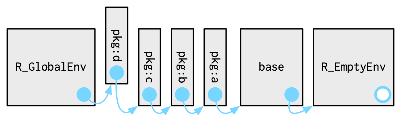
An environment in R is a data structure R uses to keep track of the names of objects and where those names resolve to values.
R creates several kinds of environments with distinct roles in execution and name lookup.
R creates the base environment, (base_env()) when it starts.
The base environment is the foundational environment of R.
R then creates the global environment (global_env() or .GlobalEnv) as a child of the base environment.
As discussed in Section 5.3, when a function object is created, R stores a reference to the current environment and that reference becomes part of the function object.
As a result, every function has a function environment, also called its enclosing environment
The function (enclosing) environment has several key properties:
Lexical scoping is a computer science term that means a function resolves names (the lexicon) based on the scope of where it was defined, not where it is called.
Every environment in R contains a reference to another environment, accessible via parent.env().
In most cases, the parent and enclosing environments refer to the same environment but have distinct roles:
parent.env().
parent.env() is historical. It exposes the pointer used for lexical scoping, but the concept it represents is more accurately described as the enclosing environment.Every R package has a namespace, which is implemented as a special kind of environment.
The namespace environment contains all objects defined by the package:
Two special characteristics are:
Execution environments exist only while code is running.
They are central to understanding how R evaluates expressions and how debugging works.
The current environment, or current_env(), is the environment in which R is currently evaluating code.
The calling environment is the environment from which a function is called (invoked).
All functions in R execute inside their own environment.
When a function is called, R creates a new execution environment, also called a frame, and evaluates the function body inside it.
A frame contains:
Frames are:
At any moment, exactly one frame is the current environment.
A function’s enclosing environment is a structural property of the function object, whereas a frame is an execution environment created at call time.
So far, we have distinguished between:
Two additional constructs connect these environments into a working system: the search path and the call stack.
The search path is an ordered list of environments that R consults after lexical scoping when resolving names in interactive use.
search() or examine in RStudio/Positron using the drop down next to Global Environment.
search() returns a character vector with the Global Environment as the first element and the Base Environment as the last.When R starts, it initializes the search path with the Base Environment and the Global Environment.
When a package is attached using library() or attached(), R inserts the packages package environment into the search path immediately after the Global Environment.
When RStudio opens or restarts an R session, R itself automatically attaches several base packages that support interactive work (including {methods}, {utils}, {datasets}, {grDevices}, {graphics}, and {stats}).
In addition, RStudio attaches its own IDE-managed environment called “tools:rstudio”, which supports editor, help, and debugging features.
search().When resolving a name after lexical scoping has been exhausted, R consults the search path in the sequence
This sequence explains why functions from attached packages can be called without qualification (e.g., lm() instead of stats::lm).
detached()), it can still be found using the :: operator.Important distinctions:
The search path determines which attached environments are visible by name, while lexical scoping determines how functions resolve names during execution.
The call stack is the ordered sequence of active frames created by nested function calls.
The call stack therefore records how execution arrived at the current point, not how names are resolved.
Key properties:
Debuggers display the call stack so you can see who called whom.
Evaluating an expression of the form function_name() causes R to:
Nested calls create multiple frames, which together form the call stack.
Listing 5.1 demonstrates lexical scoping for function f.
In this example, the global environment is the enclosing environment of f(), because f is defined at the top level of the document.
What happens when g() is called:
g() (this frame is the calling environment of f()).g() calls f(1) and creates a new frame for f().f():
x is found in the f() frame.a is not found in the f() frame R uses lexical scoping and looks next in environment(f) (the enclosing environment) and finds a <- 1.g() (the calling environment) defines a <- 10, that value is not used.In the previous example, the enclosing environment of f was the global environment because f was defined at the top level.
In Listing 5.2, f is defined during execution, inside the make_f function, so its enclosing environment is not .GlobalEnv.
f() captures a from its enclosing environment.
1make_f <- function() {
  a <- 10
  f <- function(x) {
    x + a
  }
  f
}

f2 <- make_f()
a <- 1
f2(1)make_f: R creates a function object with formals: (), a body (the code block), and an enclosing (closure) environment: the current environment at definition time (here .GlobalEnv)
a or f exists yet.make_f(): R evaluates the call to make_f() and creates a frame for this call. That frame has bindings for the formal arguments (here: none) and a parent/enclosing link to environmnet (make_f) (here: the Global Environment).
make_f frame on top of the call stack as the current frame.a <- 10: As that line executes, R adds a binding in the make_f frame with name a and value - a pointer to the object 10.f <- function(x) { x + a }: R evaluates the function (x) {ax + a) expression which creates a new function object in the make_f frame with formals (here x), body (x + a) and the enclosing environment of the current environment which is the make_f frame.
<- binds the name f in the make_f frame to the new function object. 5.Evaluate f as the return value: The last expression in make_f()is f (which is not a call to f), so R returns the function object bound to f and then the call finishes:f2 in .GlobalEnv.make_f frame from the call stack.make_f() frame is not “garbage-collected” as f contains a reference to it. f2 is not a copy of f but is another name bound to (referring to) the same objectf2(1): R creates a new frame for f2, binding x = 1 and the parent/enclosing environment of the make_f frame.
f2 frame onto the call stack as the current frame.x+ a.x is found in the f2()’ frame.a is not found in the f2() frame so R looks in the enclosing environment of f2() and finds a = 10.1 + 10 and returns 11f2 frame from the call stack.The result is: 11
The previous examples resolve a via lexical scoping (frame to enclosing environments ).
The example in Listing 5.3 shows what happens when a name is not found in lexical scope and R then consults the search path.
What happens when h() runs:
h() and binds argument x.var(x) requires resolving the name mean:
var is not found in h()’s frame,var is not found in environment(h) (typically .GlobalEnv),var in base R’s attached environments (ultimately the stats package/namespace).var was not defined locally.During debugging, tools like browser() pause execution inside a specific frame, the current frame.
The current frame determines:
The call stack is the sequence of frames that led to the current one.
traceback() prints the call stack up to point of error, usually shown after an error or during debugging.We will refer to these execution environments explicitly as frames when discussing interactive debugging.
For a deeper treatment of environments see Advanced R, Chapter 7
Everything that happens in R is a result of a function call, but not all calls look the same.
Function calls come in four varieties:
foofy(a, b, c).
x - y.
%.names(df) <- c("a", "b", "c").
[[, if, and for.
While there are four forms, you actually only need one because you can write any call in prefix form and it’s the most common.
Prefix calls allow you to specify arguments in three ways:
help(mean).help(top = mean).help(topic = mean).Arguments are matched by exact name, then with unique prefixes, and finally by position.
List of 3
 $ a : num 1
 $ b1: num 2
$ b2: num 3List of 3
$ a : num 1
$ b1: num 2
$ b2: num 3List of 3
$ a : num 1
$ b1: num 2
$ b2: num 3Error in `k01()`:
! argument 3 matches multiple formal argumentsPrefix form is what allows functions to change other functions by manipulating their arguments programmatically.
Some Best Practices for working with arguments.
warnPartialMatchArgs option:As discussed in Section 5.5.1.3, when evaluating a function, R resolves names using “Lexical Scoping.”
There are four primary implications for how functions are evaluated:
Try to figure out what value the following will return before you run it.
If a name is not defined inside a function, R looks in the function’s enclosing environment.
When a function is called, R looks first in function’s current frame for names.
not found error message.Look at help for mean().
x (for the data object).x is defined in the mean() function, R looks no further and it does not care that you may have a variable called x in your Global Environment.x to the function variable x and uses its own x in executing the function.Run the following code in your head. What is the result? Then run the code to check your answer:
Functions are ordinary objects so the scoping rules (name masking) also apply to functions.
[1] -90[1] 0When a function and a non-function share the same name (from different environments), it gets complicated.
To minimize issues with names and scoping across levels:
x, or y and df for data frame or otherwise names specific to that function.Every time a function is called, R creates a new execution environment to host its execution.
Lexical scoping determines where, but not when, to look for values.
[1] 14[1] 19Use codetools::findGlobals() to list all the external dependencies (unbound symbols) within a function:
A drastic approach to check things is to manually change the function’s environment to the emptyenv(), an environment which contains nothing, to include the primitive operators like +:
What value does the following function return? Make a prediction before running the code yourself.
R uses lazy evaluation of function arguments; they’re only evaluated if accessed.
x is never used:Lazy evaluation is powered by a data structure called a promise, or (less commonly) a thunk.
x - y, which gives rise to the delayed computation.When an argument expression includes an assignment (e.g., y <- 1000), that assignment is evaluated in the calling environment as part of argument evaluation, not inside the function body.
Calculating… printed once in the following example.[1] 60 60You cannot manipulate promises with R code They are behind the scenes.
Lazy evaluation means default values can be defined in terms of other arguments, or even in terms of variables defined later in the function.
The evaluation environment is slightly different for default and user-supplied arguments
The following is an extreme example using ls(), which returns a character vector of the names of the objects in the specified environment:
 [1] "exp_x"             "f01_sin"           "f01_sin_backslash"
 [4] "f01_sin_emb"       "f01_sin_oneline"   "f02_add"
 [7] "g02"               "g03"               "g07"
[10] "g08"               "g11"               "g12"
[13] "h01"               "h02"               "h03"
[16] "h04"               "h05"               "k01"
[19] "sum_ex"            "triple"            "x"
[22] "y" [1] "a" "x" [1] "exp_x" "f01_sin" "f01_sin_backslash"
[4] "f01_sin_emb" "f01_sin_oneline" "f02_add"
[7] "g02" "g03" "g07"
[10] "g08" "g11" "g12"
[13] "h01" "h02" "h03"
[16] "h04" "h05" "k01"
[19] "sum_ex" "triple" "x"
[22] "y" To determine if an argument’s value comes from the user (FALSE), or from a default (TRUE), you can use missing()
List of 2
 $ : logi TRUE
$ : num 10List of 2
$ : logi FALSE
$ : num 10missing() is best used sparingly.... (dot,dot,dot) ArgumentFunctions can have a special argument, ..., which allows the function to take any number of additional arguments.
map().purrr::map() or 't.test().return()A function can return a value either implicitly or explicitly
return().Explicit is much more user-friendly and helps in debugging and maintaining functions of any length
return() to be explicit about what could happen.There are two approaches:
retun() everywhere you plan for a return.return() at the end. That can make it easier to troubleshoot.return() for each possible ending, and,return() at the end.[1] FALSE FALSE FALSE[1] TRUE FALSE TRUE## Use of intermediate variable for the return value
## with only one `return()`
has_name <- function(x) {
nms <- names(x)
if (is.null(nms)) {
my_return <- (rep(FALSE, length(x)))
} else {
my_return <- (!is.na(nms) & nms != "")
} ## end else block
return(my_return)
} ## end function
## test our function
has_name(x1)[1] FALSE FALSE FALSE[1] TRUE FALSE TRUEMost functions return visibly: calling the function in an interactive context prints the result.
You can prevent automatic printing by applying invisible() to the last value:
To verify this value does indeed exist, you can explicitly print it or wrap it in parentheses:
The most common function that returns invisibly is <- which means you can chain assignments without lots of intermediate results.
If a function cannot complete its assigned task, it should throw an error with stop(), which immediately terminates the execution of the function.
An error means something has gone wrong, and forces the user to deal with the problem.
A primary place for error checking is immediately after the function is defined where you evaluate the class/type, length, and value constraints of each argument.
Two common approaches:
stop() to create a custom error message.stopifnot() will stop execution if any of its argument expressions evaluate to FALSE and then provide a generic error message based on the first FALSE argument.my_fun <- function(df, y = "cat", z = TRUE){
stopifnot("Input df is note a data frame" = is.data.frame(df),
"Input y is not character" = is.character(y),
"Inout z is not logical" = is.logical(z),
length(df) > 2, length(y) == 1, length(z) == 1,
"data frame must have more than one row" = nrow(df) > 1)
c(names(df), y)
}
my_fun("cat")Error in `my_fun()`:
! Input df is note a data frameError in `my_fun()`:
! Input y is not characterError in `my_fun()`:
! Inout z is not logicalError in `my_fun()`:
! length(df) > 2 is not TRUEError in `my_fun()`:
! length(y) == 1 is not TRUEError in `my_fun()`:
! length(z) == 1 is not TRUEError in `my_fun()`:
! data frame must have more than one rowBoth options evaluate the arguments and tests one at a time and stop at the first error.
Keep in mind: stop() is usually executed after an if statement condition is TRUE, whereas stopifnot() executes if any one of the conditions is FALSE.
function() function by using <-.,
my_function_name <- function(x,y,z){} where x, y, z represent your arguments (if any){}.
\(df) nrow(df), you do not need the {}.{.} on its own line.|> or %>%) or inside ggplot() the + with no trailing spaces.return() to explicitly identify the source of the return value (the output result) of the function.stopifnot() for rapid checking of multiple conditions for the arguments with simple error messages.if style statements.You can always reuse a custom function in the same document in which it is defined.
If you want to reuse your function in another document or analysis, write your function in a .R file, with only code and comments, no markdown, in what is known as an R Script file.
/R directory.To make the function available in other files (.qmd or .R), you have to “source” it in each file.
source() evaluates the file in the current environment (by default).To source the geometric mean R script in this file (so I can use the function in the script), enter:
geo_mean() function … with a caveat about dependencies.If an R script uses a function not in Base R but from another package, e.g., %.% or ggplot(), then it depends on that package being available in the current environment.
Managing these kinds of package dependencies is a major responsibility of R Packages.
To use the geo_mean() function we have to load the {magrittr} package to get access to the %>% pipe operator.
Not having to load extra packages is one reason why using the Native Pipe, |>, if appropriate, is more convenient for functions you want to share across documents or with others.
It also helps when writing functions for use by others to fully specify the function using package name and the namespace-dblcolon operator, :: as in package::function().
While a README.md file is not required for an R package, most packages use the usethis::use_readme_rmd() function to generate a .Rmd file as a skeleton.
If you are pushing your functions into a GitHub repo that is Not a package, you can also create a README.md to describe your repository.
GitHub only renders a lean version of markdown often referred to as GitHub Flavored Markdown (GFM) that does not support all the features of Quarto Markdown.
README.qmd can include executable R code, figures, captions, and cross-references and still be converted to a .md file that supports GFM.README.qmd file when the following YAML is included:format:
gfm: default
html:
embed-resources: trueAfter adding this YAML, render the file from the terminal.
quarto render README.qmd --to gfmquarto render README.qmd --to htmlQuarto will generate the HTML that is required to represent links and captions in GFM.
Once you push your repo to GitHub you should see the rendered README.md displayed on the repository’s main page.
GitHub will convert the README.md file into HTML to be displayed in the browser.
It can display static images (e.g., .png or .jpg) embedded from a directory using the Markdown  syntax.
It can also display figures generated from code such as plots.
To see captions in GFM format, you must use cross-references as a workaround to set the Pandoc attributes.
To overcome limitations in GFM, the {knitr}-Pandoc process used by RStudio to create the .md file has a few extra steps behind the scenes.
 to the alt-text for an HTML image as it does not support captions directly.{#fig-my-figure-cross-reference}, right after the image R Markdown, e.g., ![](){#fig-my-figure-cross-reference}, Pandoc will convert the “[caption-text]” into an element below the image with CSS ID from the attribute and CSS class “.caption” and add to the .md document.<figure id="fig-vars-df-debug" style="text-align:center;">
<img src="./images/vars_df_debug.png"
alt="Example of using a break point to debug for vars_df()"
style="max-width:80%; border: 1px solid #ccc; border-radius:8px;">
<figcaption style="font-style: italic; color: #555;">
Example of using a break point to debug for <code>vars_df()</code>.
</figcaption>
</figure>#fig-vars-df-debug as in “See Figure 7”You can use a README.qmd file and render it to produce a README.md file with associated images ready to display in GitHub.
.md file the way it can with an HTML output.README_files directory and create markdown links to the images in the .md file.Create a file called README.qmd at the top level of your repo.
Use the following YAML header.
{#fig-cross-ref-label}.#| label: fig-my-figure#| fig-cap: My plot of diamonds.README.md document. It will also create a folder called README_files and place any code-generated images there.README_files folder..gitignore files include a line like *_files/ to avoid moving temporary files to GitHub. However in this case we want them.*_files/ that is !README_files/ and save the .gitignore file.README.md information at the bottom.It is good practice to add documentation to your function to answer at a minimum:
You can just manually use # to put comments in front of your file to answer these questions but there is a better, more standardized approach in R.
The {roxygen2} package allows you to create consistent help documentation for functions for use by you and eventually others.
install.packages("roxygen2")function() functionInsert Roxygen Skeleton.#' Title
#'
#' @param x
#' @param y
#'
#' @return
#'
#' @examples
my_fun_name <- function(x, y) {
}A best practice for code development is build-a-little, test-a-little, commit-a-little to minimize the need for debugging large chunks of code.
str(), class(), head(), names(), dim(), dplyr::glimpse(), View().If your code only works without restarting R, it doesn’t work reliably. Restart the session periodically and rerun from the top to verify reproducibility.
You’ll move faster if you label the failure mode up front.
The following list moves from typically simple errors to more complex errors to resolve.
mutate() on a factor; UseMethod() errors)NA/NaN/Inf; length mismatch; join creates 0 rows)Debugging is not guessing.
Use the least effort tool that can resolve the problem and escalate as needed.
browser()/debugonce()/debug())Integrated Development Environments (IDEs) provide early indicators for common parsing issues such as missing parentheses, unbalanced braces, and incomplete expressions that keep your code from parsing correctly.
Common signs your code does not parse cleanly.
+) after you submit code.If you see the console prompt change to +, stop and fix structure first.
), }, ], or quotes.R provides three different kinds of feedback.
Don’t ignore or suppress warnings or errors on new code. Check that they are not suppressed in code with errors.
Messages, warnings, and errors do not detect logic errors if the code is syntactically valid and “acceptable” to R. You must check outputs for reasonableness.
Before you “debug deeply,” confirm you are calling the intended function with the appropriate arguments.
The help document for a function can be considered a “contract with the user” about the function’s syntax
The help page tells you the package the function came from so you can check the package to see if there are any vignettes that might be helpful, e.g., vignette("dplyr").
Namespace conflicts and function name masking can lead to calling a different function than you think.
find("filter") or find("select") to see where a name is found.conflicts() to see common collisions.dplyr::filter() or stats::filter().Many base functions are generics that call other functions/methods based on the class of the arguments. The generic help is usually less useful than the method help.
summary look for summary.lmmethods() function, e.g., methods("plot") or methods("print"), to show all the methods, you’ll see the plot.lmgetS3method("plot", "lm") to inspect the method, if needed.?pkg::fn when you want the contract for a specific function.Check what the function expects.
NA values).Many “mysterious” errors are syntax “contract” violations.
When you encounter an error, your first goal is to verify that the objects flowing into the failing code are what you think they are
Start by inspecting the objects nearest the error.
class(x)str(x) (for deeply embedded lists, subset the data to a few top level elements to avoid seeing all the data).length(x)names(x)dim(x), nrow(x), ncol(x)head(x)summary(x) for numeric-like objectsanyNA(x) and is.na(x) for missingness checksglimpse() to inspect data frames structure and classesview() or View() to inspect data frames or tibbles visually; useful for values, but not reliable for structure as list-columns and attributes may be flattened or hidden by the IDE for better viewing of values, so confirm structure with str().A very large fraction of debugging time is saved by running class(), glimpse() and str() early.
Once you understand the current object state, reduce the problem so the failure is fast and repeatable.
CMD Shift C, to narrow down the relevant lines.class(), str(), names(), and dim().To simplify further:
Example pattern:
R provides built-in debugging tools that work in any R environment, including the plain R console, RStudio, and Positron.
These tools expose what R was doing at the moment an error occurred and help you determine where execution failed and why.
As discussed in Section 5.6.2, the call stack is the ordered sequence of active frames created by nested function calls.
After an error occurs, you can examine the call stack to identify:
R provides functions that allow you to inspect the call stack immediately after an error, which is often the fastest way to locate the frame most relevant to the failure.
traceback() (base R)traceback() shows the sequence of calls that led to the error.
rlang::last_trace() for tidyverse-style errorsMany modern R packages, especially those in the tidyverse, use {rlang} to generate structured errors.
As a result, when working with tidyverse code, you are often already seeing an rlang-powered error report when the error occurs.
The rlang::last_trace() function complements this behavior by allowing you to re-open, inspect, and control that same trace after the fact.
rlang::last_trace() displays the execution trace leading to the error, including:
The advantage of rlang::last_trace() is not that it always shows more information, but that it presents information in a way that is faster to interpret.
rlang::last_trace() preserves and labels these intermediate frames so you can see how execution reached the failure without scanning unrelated frames.
mutate(), summarise(), filter()), even when the underlying issue occurred earlier during expression evaluation or data masking..
rlang::last_trace() makes it easier to identify the earliest frame that still involves your code, rather than stopping at the surface-level verb.rlang::last_trace() exposes where name resolution and expression evaluation occurred, which is often hidden in base traceback() output.rlang::last_trace() can be more user-friendly compared to traceback().
rlang::last_trace() helps you understand how R got there.
If a tidyverse error prints a clear diagnostic summary and the cause is obvious, you may not need rlang::last_trace() at all.
If the error is unclear, scrolls away, or involves mapping, grouping, or nested evaluation, rlang::last_trace() is usually the fastest way to regain context.
If you find yourself scanning many frames in traceback()to locate the real problem, switch to rlang::last_trace() and focus on the last frame that still involves your code.
Let’s use the following example to examine traceback() and rlang::last_trace().
$ok
# A tibble: 3 × 2
x z
<int> <dbl>
1 1 2
2 2 3
3 3 4
$bad
# A tibble: 3 × 2
y z
<int> <dbl>
1 1 5
2 2 5
3 3 5traceback() and you should get 25 calls with lots of details and you have to search for the actual error (in frame 16).
When a tidyverse or purrr error occurs, the rlang backtrace is designed to help you locate the problem quickly, but only if you read it in the right order.
Use the following steps.
purrr::map())mutate(), summarise(), filter(), or another verb applied to your objectrlang::abort(), cli::cli_abort(), .handleSimpleError(), or withCallingHandlers().Run rlang::last_trace() and you can see the summary identifies the error and as you follow the black lines you get to line 13 where the error occurred.
<error/rlang_error>
Error:
! `d` must be numeric
---
Backtrace:
▆
1. └─global f("a")
2. └─global g(a)
3. └─global h(b)
4. └─global i(c)Each step in the trace
purrr::map(lst, function(df) mutate(df, z = x + 1)): Your top-level call that asks purrr to iterate over lst, applying a function that calls mutate().purrr:::map\_("list", .x, .f, ..., .progress = .progress) is purrr’s internal implementation of map() for lists.
map() delegates to map_() to do the actual looping and bookkeeping.
::: (triple colon operator) accesses map_)_ which is a non-exported internal function.purrr:::with_indexed_errors(...) is a purrr wrapper that adds index/name context to errors which is how purrr produces messages like: “In index: 2” or “With name: bad”.
base::withCallingHandlers(...) is base R condition-handling infrastructure used by purrr to intercept errors and attach context.
purrr:::call_with_cleanup(...) is the purrr helper with base R try() to cleanup after errors occur, e.g., ensures progress bars, state, etc. are closed or cleaned up.global .f(.x\[\[i\]\], ...) the actual .f function you supplied to map() which purrr is now calling on the ith element:
.x[[i]] is the current element (here, the data frame named bad when i = 2).f is your function (function(df) mutate(df, z = x + 1))dplyr::mutate(df, z = x + 1) is the exported mutate() generic you called which means dplyr begins evaluating your expression z = x + 1 in the context of df.
dplyr:::mutate.data.frame(df, z = x + 1) is the method that generic mutate() actually runs (dispatches) for a data frame.
dplyr:::mutate_cols(.data, dplyr_quosures(...), by) is internal code that loops over the new/modified columns.
mutate() turns your expressions into quosures and processes them column by column.
dplyr:::mutate_col(dots[[i]], data, mask, new_columns) is internal evaluation of one mutate expression (one “column”).
mask\$eval_all_mutate(quo) is the step where dplyr evaluates your expression inside the tidyverse data mask.
dplyr (local) eval() is the final evaluation call inside dplyr where base eval() is being run in dplyr’s controlled environment.
As a workflow rule: Look at a call stack trace to keep from guessing about where the error occurred.
rlang::last_trace() works whenever the package/function developer used {rlang}’s condition system to manage errors.
traceback() or use other methods such as debug() or browser()Interactive debugging lets you pause execution and inspect local state while the code runs.
Use interactive debugging when:
There are three main functions:
debugonce()debug(fn) with undebug(fn)browser()debugonce(fn)debugonce(fn) marks a function for debugging and causes R to enter “browse mode” (aka debug mode) in the console the next time the function is called, pausing execution at the start of the function.
Figure 5.2 shows how one can use debugonce(fn) in a plain R console to enter browse (debug) mode to examine a function line by line.
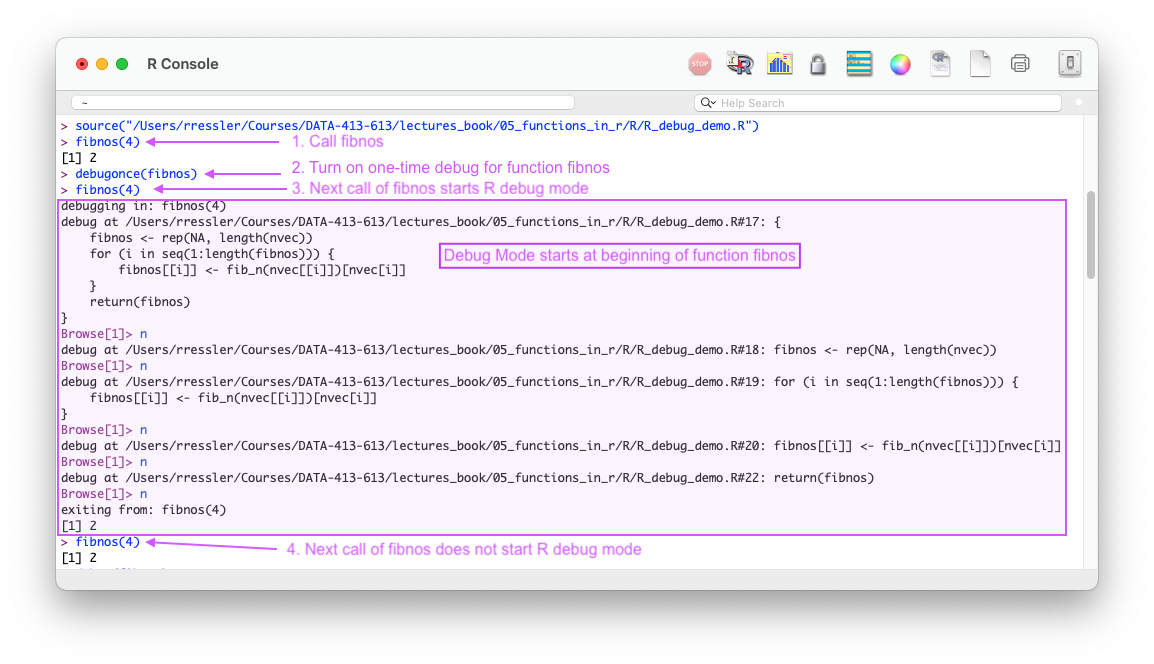
debugonce(fn) to enter browse mode only the next time the function is called.
debug(fn)debug(fn) marks a function for debugging and causes R to enter “browse mode” (aka debug mode) in the console the next time the function is called, pausing execution at the start of the function.
undebug(fn)
Figure 5.3 shows how one can use debug(fn) in a plain R console to enter browse (debug) mode every time the function is called until it is turned off with undebug(fn).
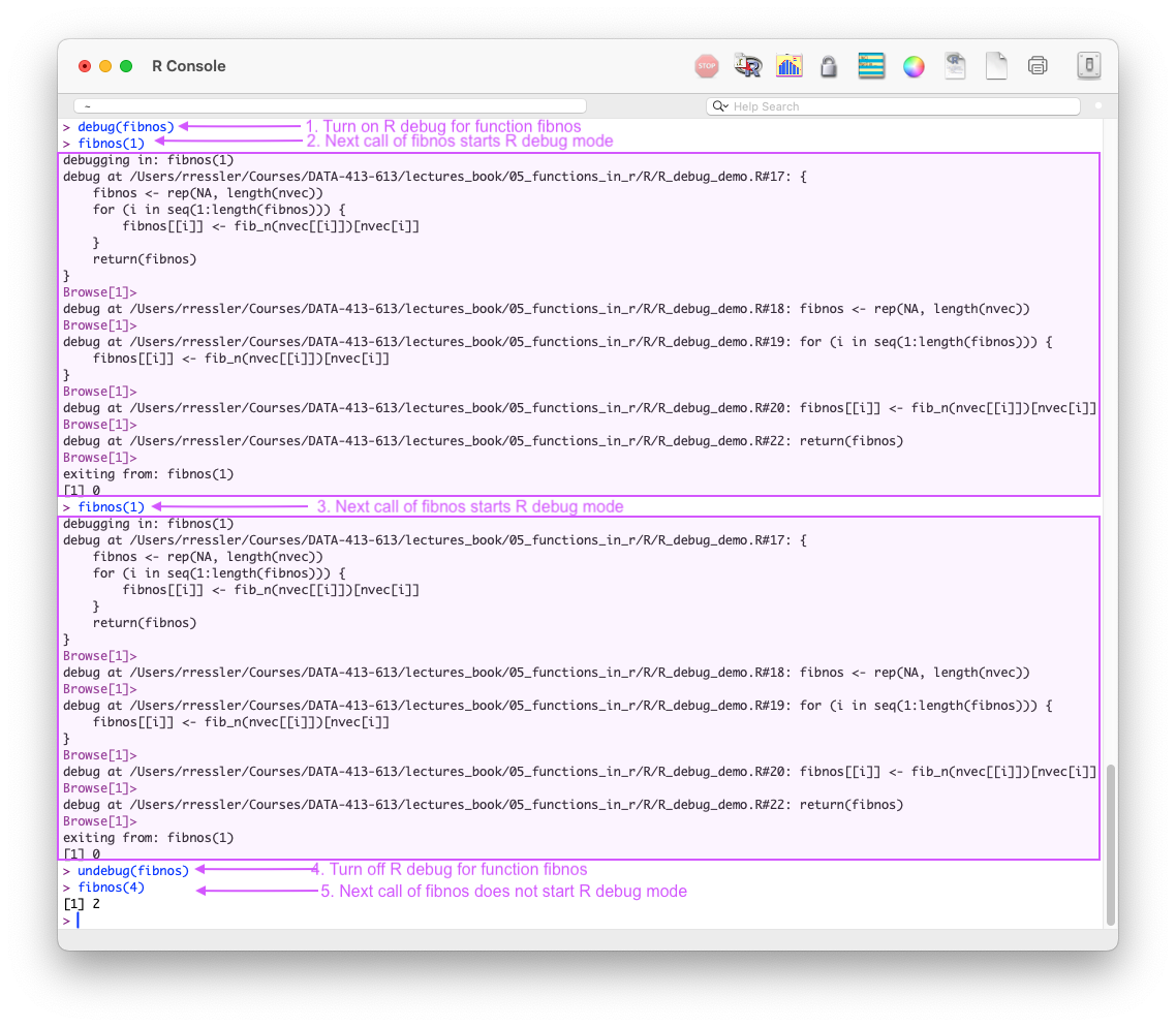
debug(fn) to enter browse mode multiple times until undebug(fn) is called.
browser()When R executes a line that contains browser(), it calls browser() like any other function.
browser() then invokes R’s interactive debugger and you enter browse mode in the console the next time the function is called, pausing execution at line with browser().
This can be useful to start the browse mode just before the line that causes the error.
R will enter browse mode every time the function is called until the browser() call is removed and the function is re-sourced.
browser() can be conditional, which is useful in loops or only-on-error situations.If statement condition to start debugging after hundreds of loop iterations when the error might first appear:Figure 5.4 shows how one can use browser() in a plain R console to enter browse (debug) mode every time the function is called until it is turned off with undebug(fn).
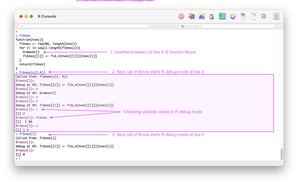
browser() to enter browse mode at specific line in a function.
Always remove or comment out calls to debug(), debugonce(), browser(), or related debugging hooks before rendering or committing or pushing code to GitHub.
When R pauses execution and the console prompt changes to “Browse[1]>”, R has entered browse mode.
In this state, you can interactively control execution and inspect the current function environment before deciding how to proceed.
Browse mode supports a small set of stepping commands that let you move through the code deliberately rather than restarting execution repeatedly.
The most commonly used commands are:
browser(), or error.
A practical strategy is to use “n” (or Enter) by default, and only switch to “s” when you see a function call you suspect contains the error.
recover() (Optional but Powerful)recover() provides an alternative form of interactive debugging when you do not know in advance where to place a browser() call.
When enabled, R will pause after an error and present a list of active frames.
Key features of recover():
Section 5.11 discussed the debugging capabilities in R that work in the plain R console.
These capabilities also work in IDEs. However, IDEs usually add visualization capabilities on top of the base R tools to make interactive debugging faster and easier for reviewing the results and stepping through the code.
Examples include:
browser() in your code).A useful way to think about it:
When paused in browse mode, RStudio expose the state of execution in multiple panes as seen in Figure 5.5.
browser(), RStudio makes an exception an highlights the browser() line.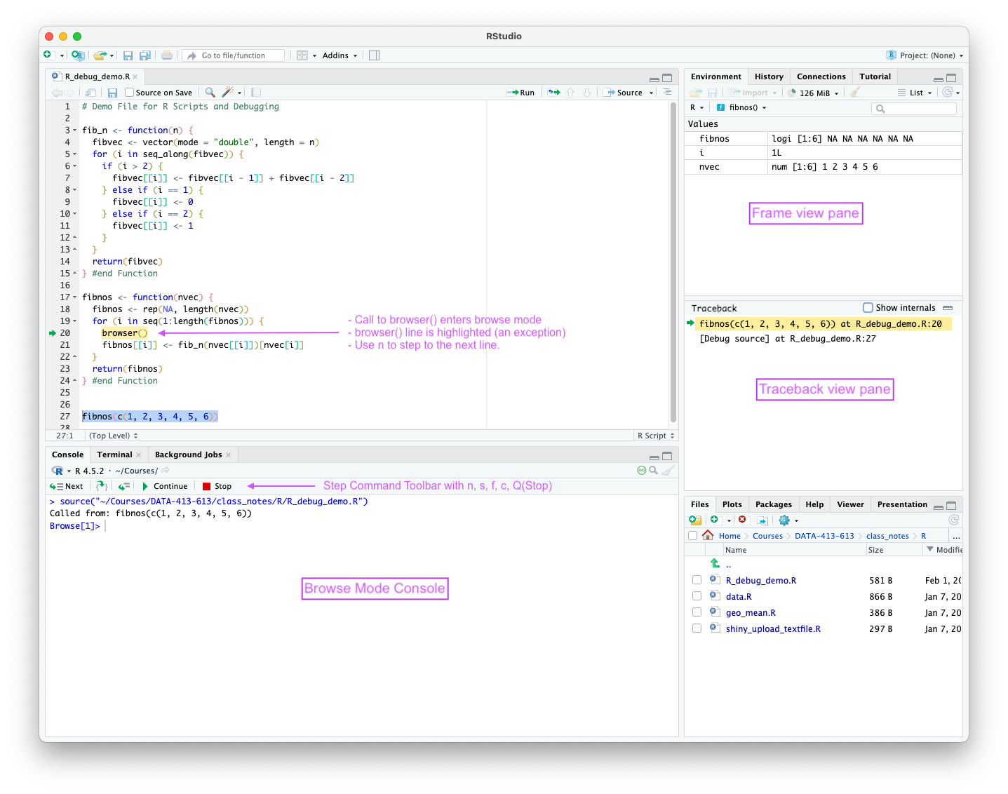
browser() line even though it has already been executed.
The RStudio console pane supports the R debug step commands using either the toolbar or the console prompt.
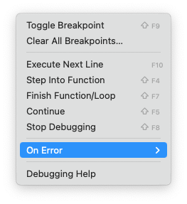
n)s)f)c)Q)The RStudio Main Menu Bar has a Debug Menu you can also use to support debugging as seen in Figure 5.6.
Entering the Browse mode using browser() is a special case as RStudio chooses to highlight the browser() command that was just executed as opposed to the next line of code to be executed.
browser() to the next line to indicate it is the next line to be executed - the usual display as seen in Figure 5.7.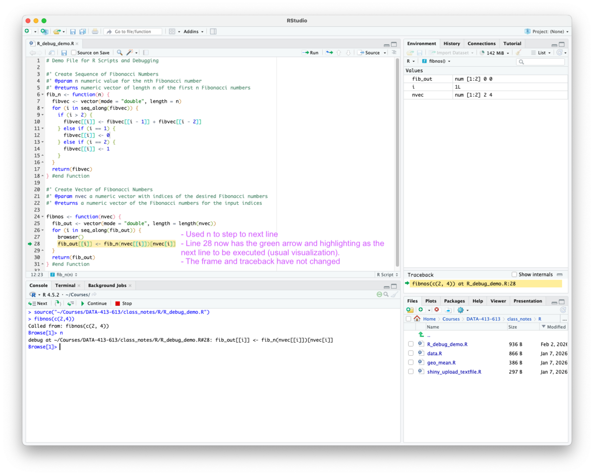
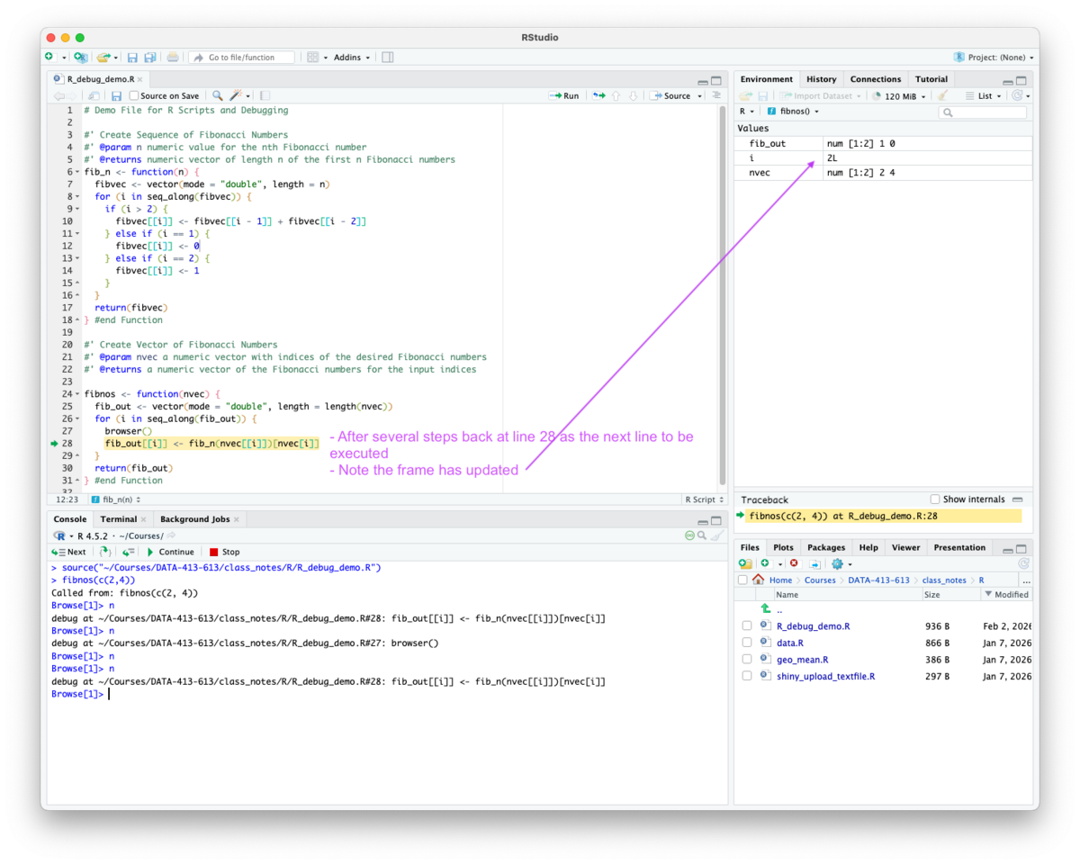
Figure 5.8 shows how the frame can change after executing several lines of code.
When using s to step into a function, the debug highlights move to the new function in the source pane and the environment/frame pane shifts to the newly-created frame for that function and adds the frame to the call stack as seen in Figure 5.9.
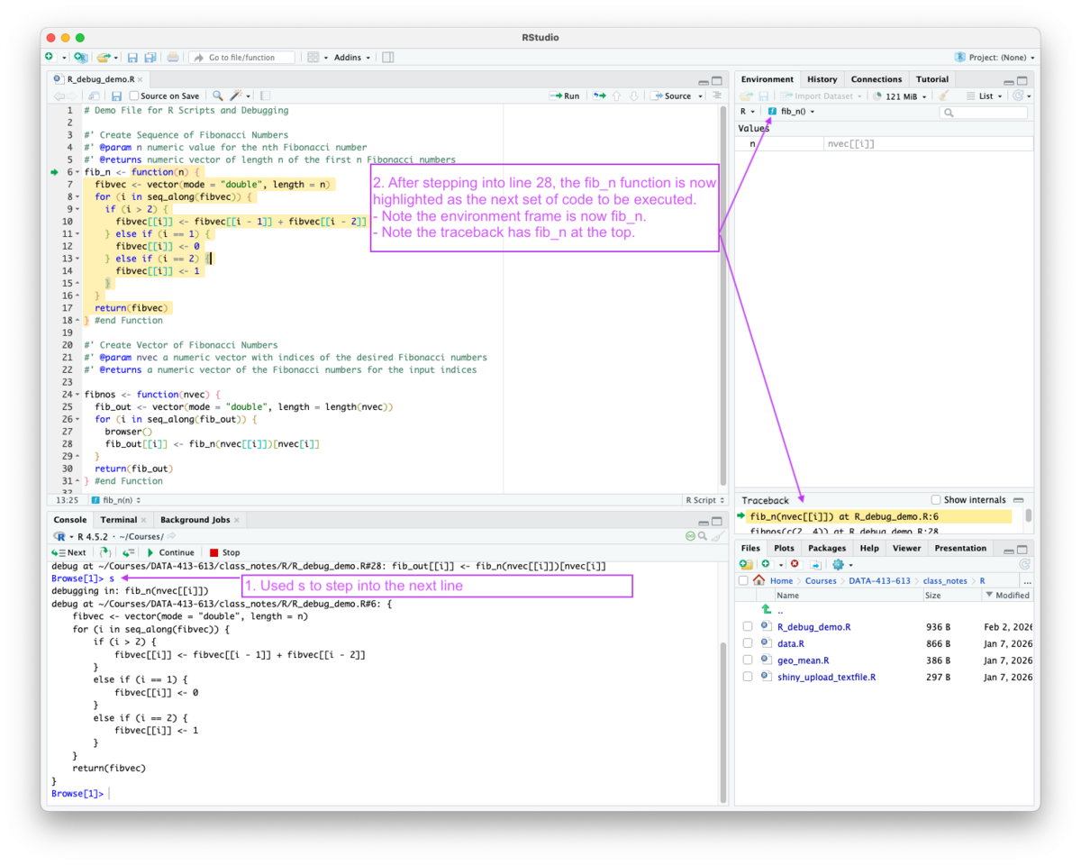
Once you have stepped into a new function, the browse mode operates as usual, with users choosing the next step, until the function returns and moves to the next call in the stack or the user selects f (to finish the function and return) or c (to continue to the next browser() or break point), or q/Stop to stop and exit browse mode.
.R ScriptsWhen you are editing a .R script file (not a .qmd or .rmd file), RStudio provides the full interactive debugging interface above and adds the ability to use visual breakpoints.
RStudio enables you to set a breakpoint in three ways:
Once you set the breakpoints the source editor should show them as open red circles as in Figure 5.11.
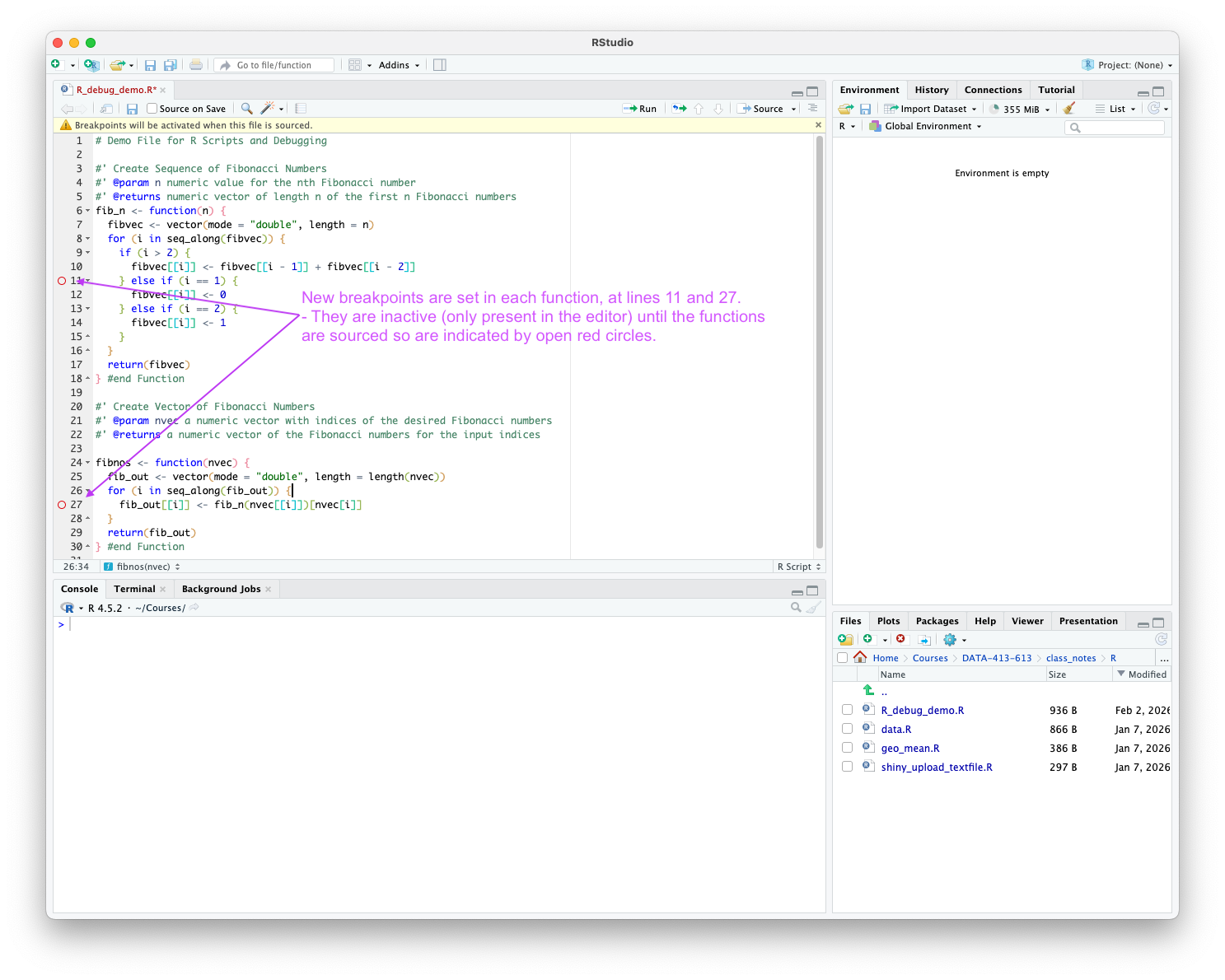
After setting one or more breakpoints:
Sourcing the script with the source icon has several results as seen in Figure 5.12.
debugSource() (a non-exported function in the {utils} package).
debugSource().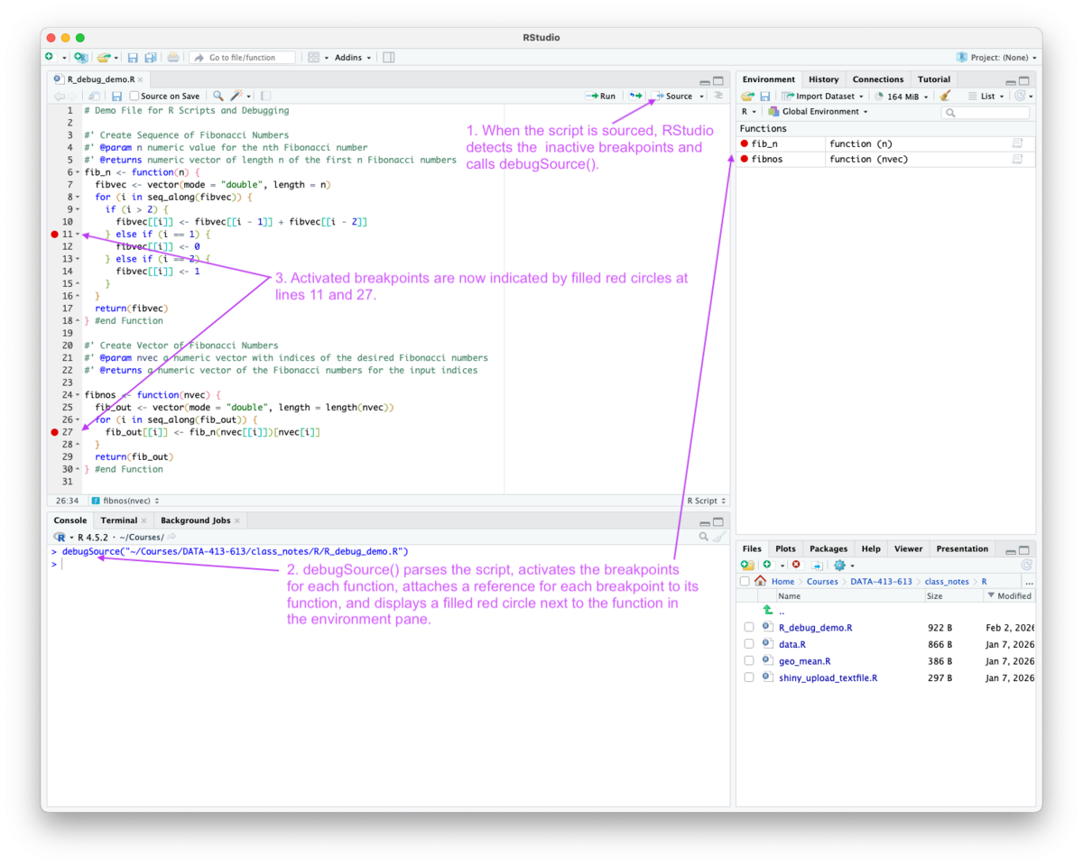
Now, whenever the function is called, it executes until it reaches the line with the breakpoint and switches into browse mode for debugging as seen in Figure 5.13.
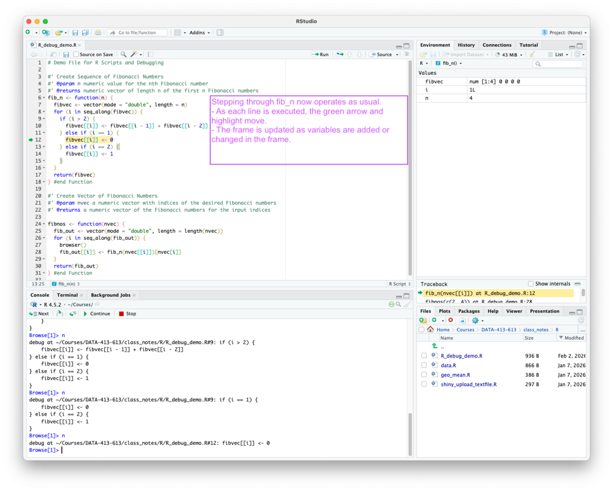
The interactive debugging operates as usual with a nuance as shown in Figure 5.14 and Figure 5.15.
for, if or else may pause execution without placing the green arrow on the breakpoint line, because the arrow can only appear on executable expressions with source references.
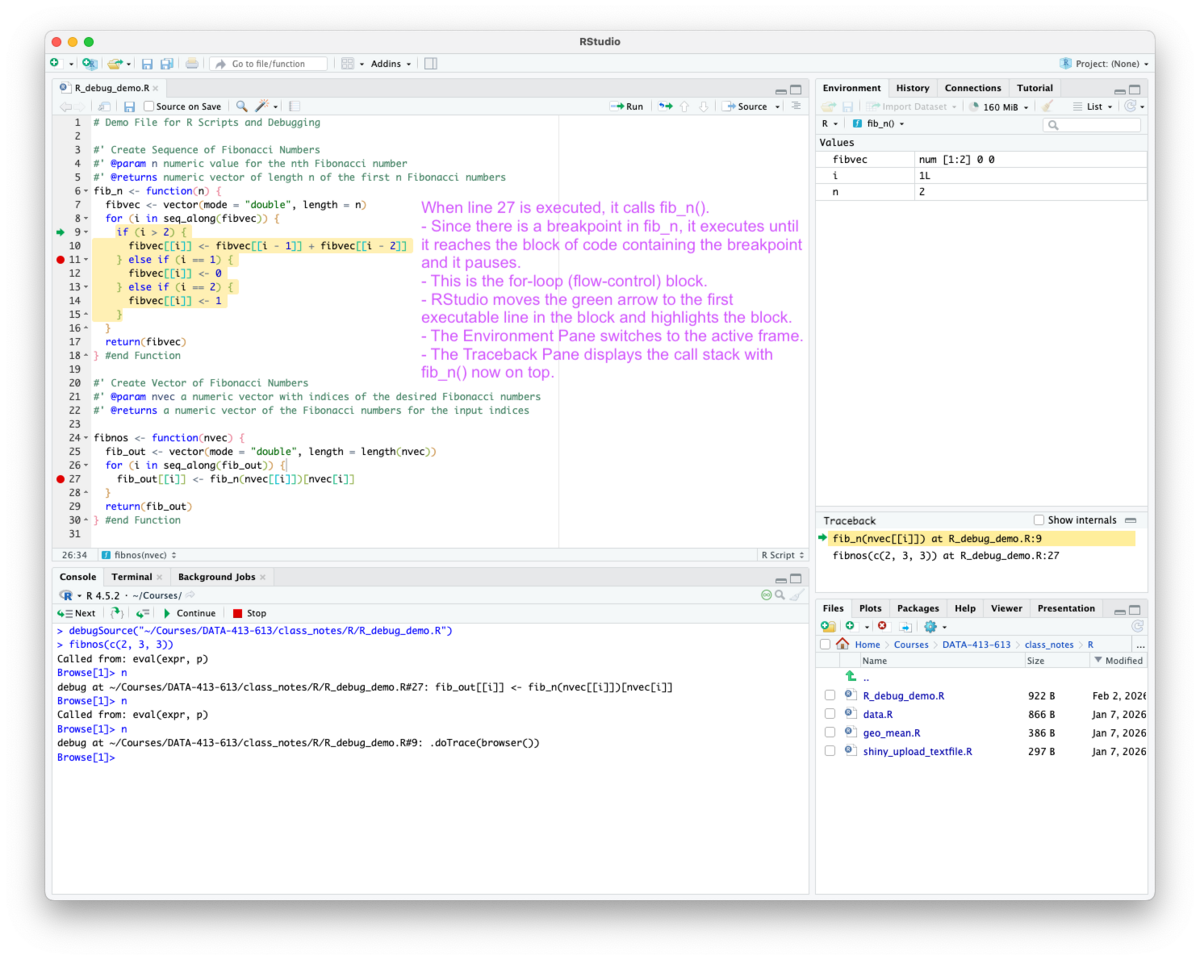
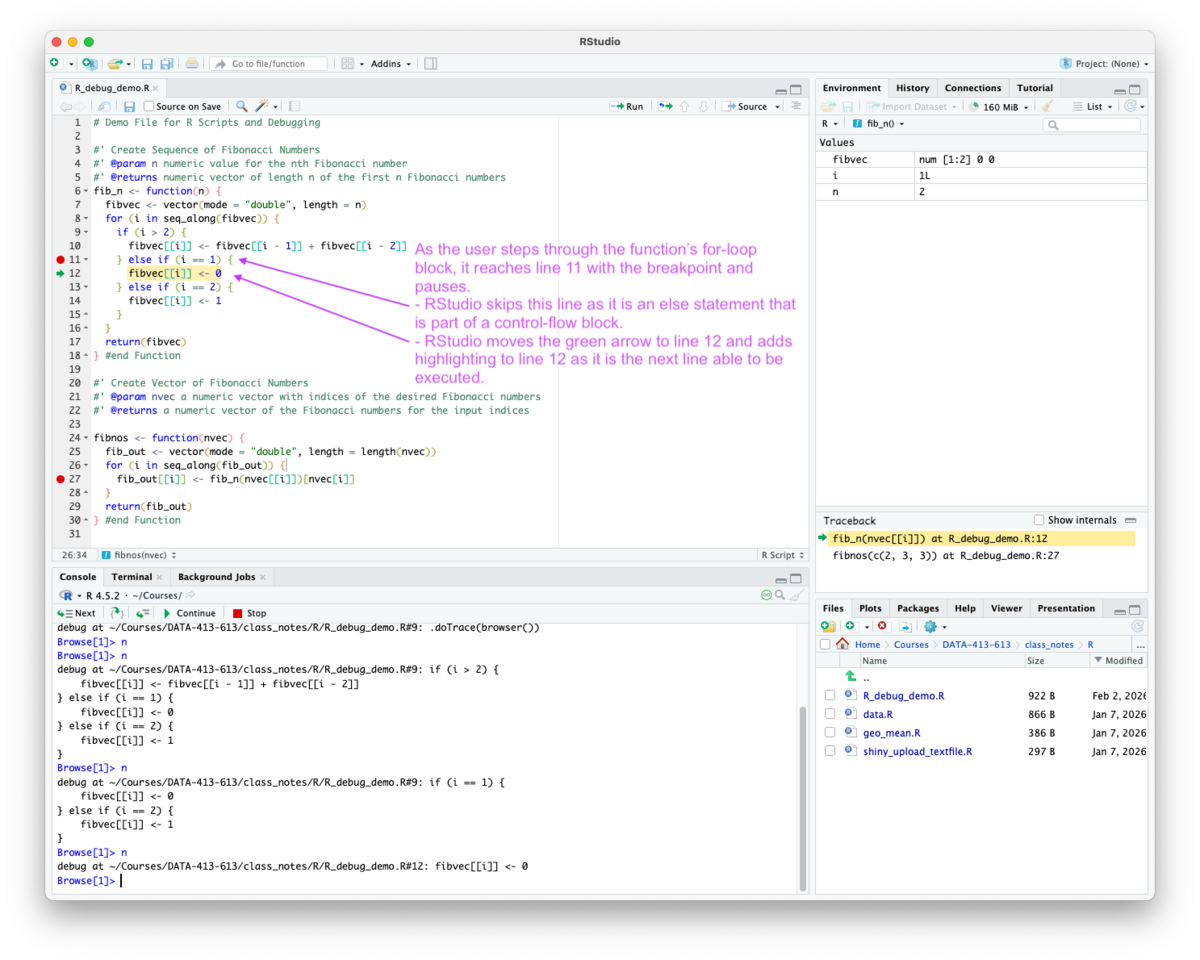
if or else statement, R may not find an executable source reference for the line so it moves the green arrow to the first executable line after the control flow statement.
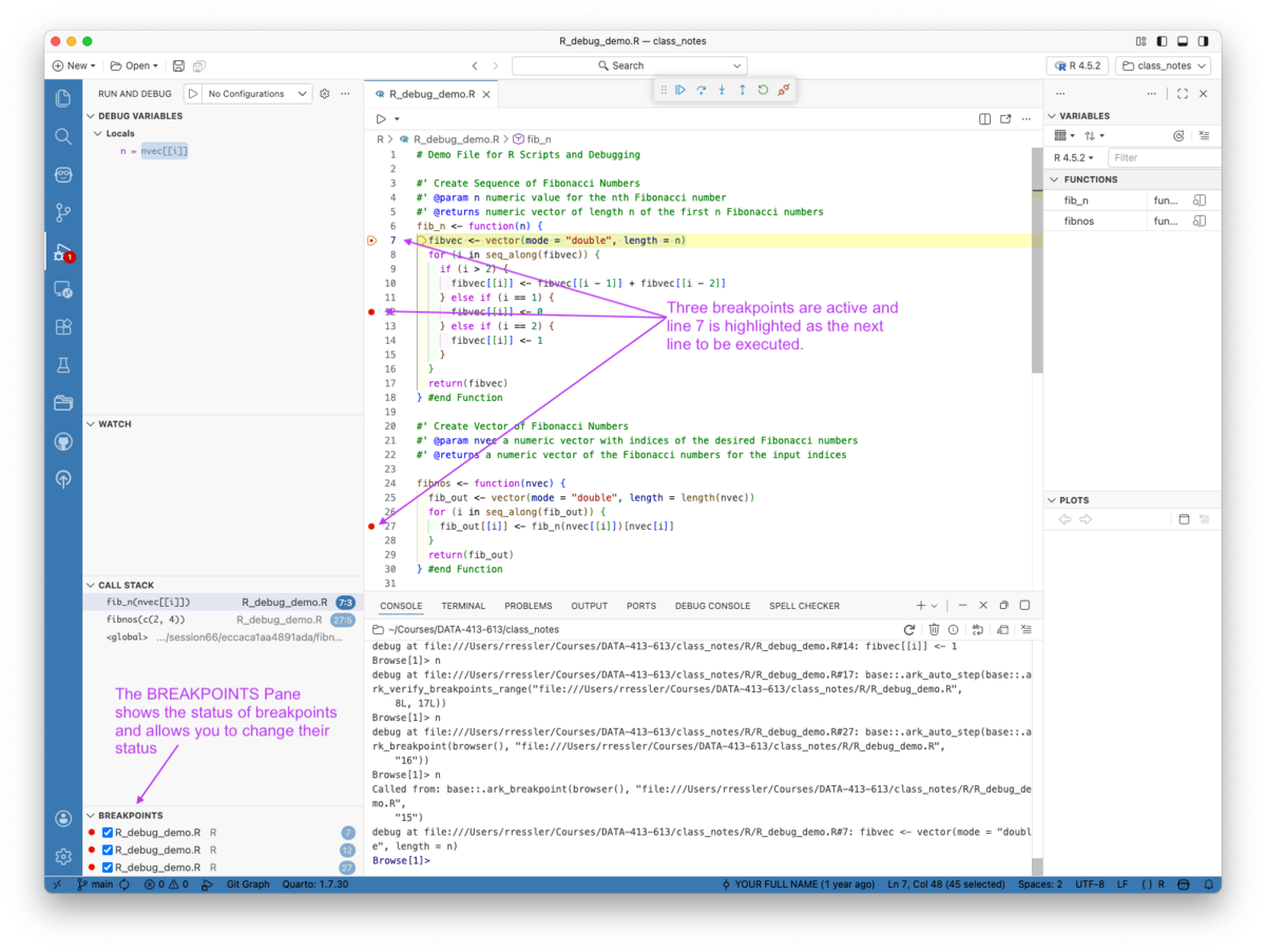
R_debug_demo.R file in the R folder.fib_n(7) to completion.
fibvec when i = 3.fibnos(c(4,5,6)).
fibnos when i = 2.Positron’s capabilities for debugging R code are based on the open-source Debug Adapter Protocol (DAP).
Positron’s R guide lists R’s four main interactive debugging capabilities:
traceback() to inspect the call stack after an error occurs,debugonce(myFunction) to step through a function call just once.debug(myFunction) to step through function calls, andbrowser() to set breakpoints in your R code,As seen in Figure 5.16, the left Activity Bar has an icon to open the “Run and Debug” pane in the Primary Side Bar.
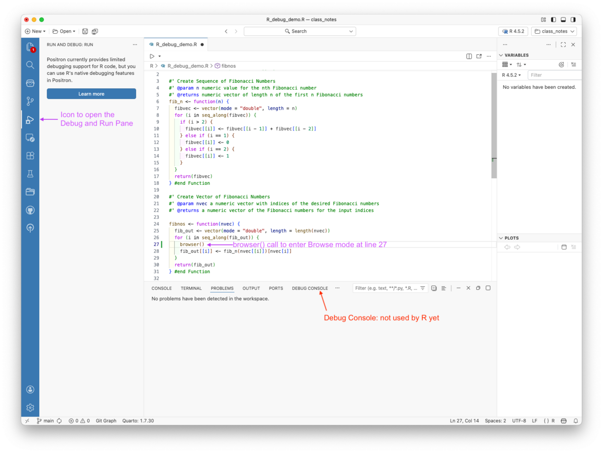
browser() where you want to pause the code and enter debug mode.browser()and enter debug mode at that point in the code.You can also use debugonce(fn) or debug(fn) with undebug(fn) without editing the function body as discussed in Section 5.11.2.
Using Breakpoints: You can now set and manage breakpoints in Positron.
When execution hits one of the functions that invoke the debug mode, e.g., browser(), R enters its native interactive debug mode as seen in Figure 5.17.
Positron then reflects the state in the Run and Debug pane. Importantly:
There are four sub-panes in the Run and Debug pane as seen in Figure 5.17.
ls() to list the objects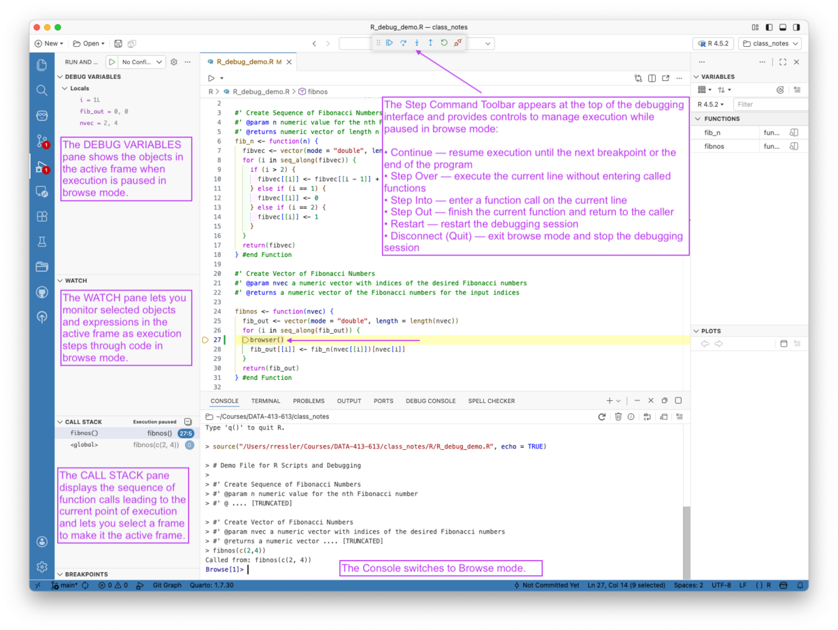
Once you are paused inside a function, you generally do four things:
Use these to answer variables pane and call stack
In browse mode, the Console evaluates expressions in the current frame. Common checks:
For data problems:
When paused, Positron supports standard R debug commands in the Console as well by using toolbar buttons at the top of Figure 5.17:
The Watch pane is designed to let you pin expressions and objects to be re-evaluated automatically each time execution is paused.
Core behavior
nrow(df), mean(x), str(obj)).This is different from the Console
Typical uses:
i, iter).length(x), dim(df)).anyNA(df), x > threshold).class(obj), str(obj)).Practical tips
In short: the Watch pane is a live dashboard for invariants and key variables while debugging—less typing, fewer distractions, clearer patterns.
You can now set and use breakpoints in R with Positron.
You can set breakpoints by
You must source or run the code to enable the Breakpoints.
Once they are active, and the function is called, you can step through the code as usual as seen in Figure 5.18
Quarto renders often run in a clean or separate process, which may differ from your interactive console session.
Key implications:
Common approach:
browser() to pause within a chunk.The {knitr} package’s purl() function extracts all the code chunks from a .qmd or .Rmd file into an R Script File (to make for easier debugging).
Run knitr::purl("path_to_qmd_file/file_name") in the console and it will create a .R file in the directory with the file name of your file and just the code from the code chunks.
The script now has access to all the interactive debug capabilities.
Shiny introduces reactive execution and additional framework stack frames.
Practical guidance:
browser() in reactive expressions or helper functions.Long-term strategy:
If the bug is still lurking, don’t be afraid to ask for help from others as appropriate to the context.
However, when asking for help, be it from LLMs, web search, or online forums, the better your question and evidence, the better and faster you can get help.
Before asking an LLM or posting online, capture:
traceback() or rlang::last_trace()str() / class() of key objectssessionInfo() for environment or version issuesTo find the root cause of an error, you may need to execute the code many times.
Create a minimal reproducible example or REPREX by copying the code into a new .R file and removing (or commenting out) code and simplifying data.
mtcars or starwars if you need other classes.If you ask for help, with a peer or online, use a Reprex or you may not get much help other than be told to submit a reprex.
Often, creating a reprex helps you locate and diagnose the error without asking for additional help.
Treat the LLM as a structured diagnostic partner, not a generic answer engine.
Good prompts include:
I am getting the following error:
Minimal reproducible example (fresh session):
Expected behavior:
Actual behavior:
Diagnostics:
Please identify the most likely root cause, propose a minimal fix that preserves intent, a more robust alternative, and 2–3 next diagnostics to run if your fix fails.
Full exception traceback:
Minimal reproducible example:
Expected vs actual behavior:
Diagnostics:
Please explain the error in plain language, propose one minimal fix, one more robust alternative, and list targeted checks to confirm the diagnosis.
Database engine and dialect:
<e.g., PostgreSQL 15>
Table schema (column names and types):
Query:
Error message:
Sample rows (anonymized):
Please identify what the engine is complaining about, provide a corrected query, and suggest validation queries (e.g., COUNT, LIMIT, EXPLAIN) to confirm correctness.
When searching the web:
The {searcher} package and the {errorist} package may help you search faster. Balamuta (2020b) Balamuta (2020a)
If you cannot resolve the issue using local evidence and targeted searching, ask for help in the right community.
When posting:
After you find and understand the error:
If you got help from the community, acknowledge the solution as correct and useful and say thank you.
Building packages is an optional topic which may or may not be covered in class or assignments.
However, since the package is the fundamental unit of shareable code in R, information in this section and its references can be helpful in understanding how the R ecosystem works.
install.packages("x").devtools::install_github("package URL")library("x").package?x and help(package = "x").install.packages(c("devtools", "roxygen2", "testthat", "knitr", "usethis"))install.packages("rstudioapi") in the console.rstudioapi::getVersion() and the date should be within the last 6 months.1 for ALL and say No to installing versions requiring compilation.Your system is ready to build packages!The structure is designed to enforce rules for working well with Base R and other compliant packages
Repositories often require specific implementations of the files to allow posting
The smallest usable package has three components:
R/ directory, with R code.DESCRIPTION file, with package metadata.NAMESPACE file.git status to check.create_package("path/packagename") to create a “skeleton” R package and invoke a new RStudio Session.
path with the relative path from the console working directory to your desired package location.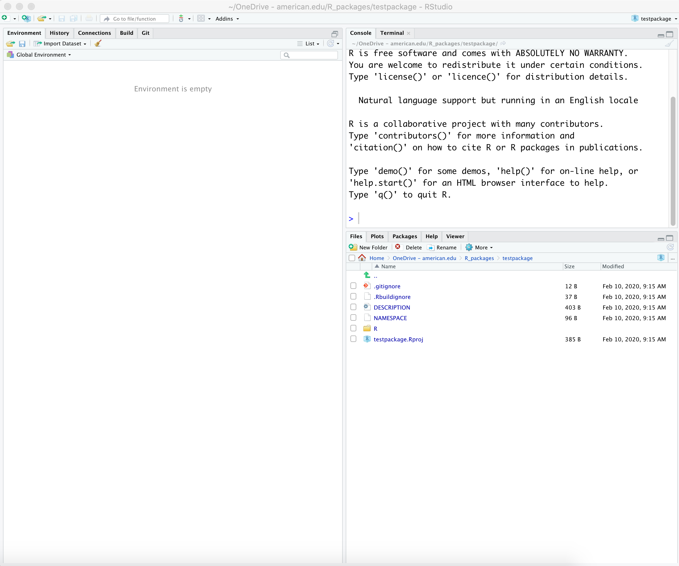
- You should see two icons for RStudio.
- The new one has the name of the RStudio Project on it..gitignore anticipates Git usage and ignores some standard, behind-the-scenes files created by R and RStudio..Rbuildignore lists files that we need to have around but that should not be included when building the R package from source.DESCRIPTION provides metadata about your package.
DESCRIPTION file.`DESCRIPTION file to be a package).NAMESPACE file declares the functions your package exports for external use and the external functions your package imports from other packages.
R/ directory is the “business end” of your package.
.R files with the function definitions for your package (or app.R files for a shiny app).packagename.Rproj is the file that makes this directory an RStudio Project..Rproj.user, if you have it, is a directory used internally by RStudio.You want to test your skeleton package to see if it will build (compile) and install properly.
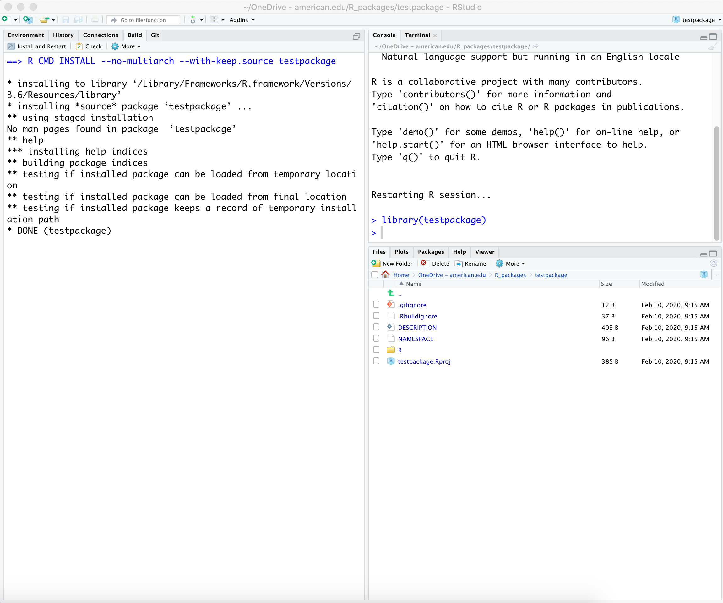
Notice, there is a new tab called “Build” in the same pane as Environment and History.
Your package is empty of code but you can test if it works from a package perspective.
Execute: In the new RStudio session go to the Build Tab (or the “Build menu”) and select “Install and Restart”
git initThe package directory is already an R source package and an RStudio Project.
Execute: Now make it a Git repository, with use_git().
.git folderCMD Shift . in Mac File ManagerDESCRIPTION file Metadata.DESCRIPTION file.
Execute: Use use_readme_rmd() and you can edit it later.
The goal of the README.Rmd is to answer the following questions for new users about your package:
On GitHub, the knitted README.md will be rendered as HTML and displayed on the repository home page.
Recommended Structure for a README.qmd:
Execute: Edit the README.qmd file to change the Installation section (lines starting with “You can install the released version of {mypackagename} from CRAN …” to something like:
install_github() function from the {devtools} or {remotes} packages.use_news_md() to create an markdown file NEWS.md you can edit.use_spell_check().If you are going to include raw data in your package or use it in developing your package, include a data-raw folder where the data is created/formatted.
Execute: Use use_data_raw()
If you are going to include processed data in your package you can use the function use_this::use_data(mydata) with the name of the data to be saved in your processing script.
data directory (if not already there) and save mydata with the desired format (e.g., .Rda) and compression.data directoryInstall and Restart in RStudio to check everything still works.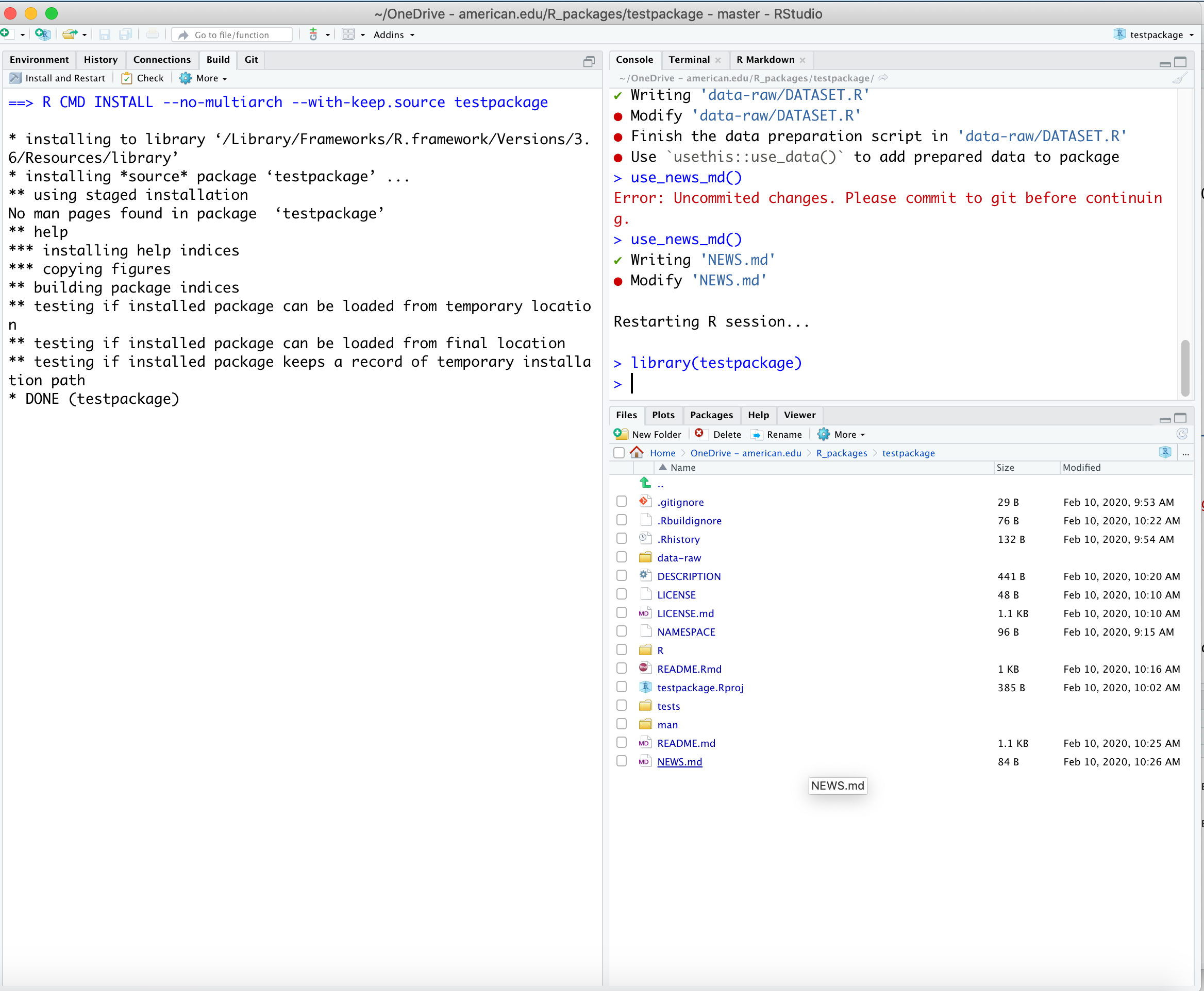
| # | Action | Keyboard Shortcut |
|---|---|---|
| 1. | Write Code and Document Functions | |
| 2. | Restart R Session | Cmd+Shift+F10 (Ctrl+Shift+F10 for Windows) |
| 3. | Build and Reload (or Install and Restart) | Cmd+Shift+B (Ctrl+Shift+B for Windows) |
| 4. | Test Package | Cmd+Shift+T (Ctrl+Shift+T for Windows) |
| 5. | Check Package | Cmd+Shift+E (Ctrl+Shift+E for Windows) |
| 6. | Document Package | Cmd+Shift+D (Ctrl+Shift+D for Windows) |
:: operator?library(devtools) in the console again.
library(devtools) in the console.
Build and Reload tests if the package works as a package - it does not check if your code makes sense.devtools::check() to run R CMD check which conducts many individual checks “using all known best practices.”
check() runs several functions to update your files and then builds your package and runs R CMD Check mypackage.tar.gzR CMD check is essential if you want to submit your package to CRAN.README and NEWS files..R/ directory (other than scripts manipulating your raw data to .RDA files in data).R directory.use_r() Function Creates or Opens any .R fileuse_r() function: use_r("file_name") ..R file or creates a new one for your function’s code.use_r() can make navigating your R files much easier when you have a lot of files.
.R directoryfbind() function.fbind() and only for fbind() in R/fbind.R and save it.source(), Use load_all() to Access the Functionsource(), we use a {devtools} function to access the function.library().load_all() to make fbind() available to other functions/scripts.fbind(as.factor(c("dog","cat")),as.factor(c("gerbil","parakeet")))load all() only simulates the process of building, installing, and attaching the new package.load_all() provides a more accurate sense of how the package is developing than creating test functions in the global workspace.
devtools::check()check() at any time to see if your package is in working order (it does not check your code for logic errors!).check() is a convenient way to run the shell command R CMD check for checking if an R package is in full working order, without leaving your R session.check() executes many checks of the code and package files for compliance with package standards.check(),
%>%)` or {ggplot2}.library() function to load (attach) other packages, they import them in a different manner.stats::median() or utils::head().:: operator or by being in the package namespace.search().library(), but that is technically imprecise.::.:: will also load a package if it is not already loaded, but it does not attach it.requireNamespace() or loadNamespace().::.
library() or require() load, then attach, the package.NAMESPACE FileWhat’s in a namespace? That which we call our function
by any other name would not smell sweet at all …
map::map() instead of purrr::map().
:: operator differentiates between functions with the same name from different packages by adding the package name to the function name.map(), but you would need to use purr::map().NAMESPACE Filecreate_package() always creates a file called NAMESPACE because it is essential for a package to work with other packages.
The NAMESPACE file is Not the namespace of the package per se, but it records the elements of the namespace for the package, which enables the creation of a functioning namespace.
Each line contains a “directive”: e.g., export(), importFrom() or others.
Each directive describes an R object and indicates if: 1. it’s exported from this package to be used by others, or, 2. it’s imported from another package to be used locally.
Execute: Look at your NAMESPACE file now.
There is no need to edit the NAMESPACE file by hand (and it’s not a good idea).
We will see later how using functions from {usethis} and {roxygen2} automatically update the NAMESPACE file based on how we identify packages and document our code.
DESCRIPTION File to Identify Needed PackagesDESCRIPTION file has a field called Imports.
create_package() does not create the “Imports” field in the bare-bones DESCRIPTION file; it assumes no other packages are needed.use_package()Imports field in the DESCRIPTION file, use use_package(), e.g. use_package("dplyr").
Imports field is not present, use_package() will add it.Imports, declares your general intent to use some functions from the exported functions in another package’s namespace.use_*() functions, e.g., use_pipe() (magritter pipe) and use_tibble().DESCRIPTION file.use_tibble() will add a file called R/mypackagename-package.R under the R directory.use_pipe() will add a file called utils-pipe.R under the R directory.R folder now to see new filesDESCRIPTION file to see the new imports fieldNAMESPACE file to see the updates from the functions.
%>% and for import for tibble()NAMESPACE will attach them to the search string so you can use them without using ::DESCRIPTION Imports field as well.
use_package("thatpackage", min_version = TRUE) to go with the current version you are using.Imports: dplyr (>= 0.3.0.1)Imports field is imprecise.
Imports field has nothing to do with functions being imported into the namespace.Imports does Not mean it will be “imported” into the namespace (attached to the search path)!NAMESPACE file.DESCRIPTION Imports field only means it must be installed (not attached) for your package to work.
DESCRIPTION Imports are installed or accessible on their computer. If not already present, it will ask to install them on their computer.
devtools::load_all() also checks to see if the packages in Imports are installed.Many users want to limit the number of packages they install on their computers and don’t like packages with lots of dependencies. So don’t add more packages than you really need to the Imports field!
It’s common for packages to be listed in Imports in DESCRIPTION, but not have a directive in NAMESPACE.
Since you may not be using a lot of functions from some packages you do not need to import/attach the whole package.
A best practice is to explicitly refer to external functions using the syntax package::function().
forcats:fcount() inside your function. This way you do not have to worry if the package is attached.:: to refer to specific packages that are installed based on the Imports field.use_package() argument type = has a default of "Imports" as the “best practice.”DESCRIPTION file has other fields for other levels of dependency, e.g., Depends and Suggests.Depends, not Imports.use_package("thatpackage", type = "Depends") to add a package to the Depends field.requireNamespace(x, quietly = TRUE)).use_package("thatpackage", type = "Suggests") to add a package to the Suggests field.use_* functionuse_package("packagename") to add the package to DESCRIPTION Imports so you know the package will be loaded.@importFrom package function1 function2 in your .R file documentation with the function names as arguments, e.g.,
@importFrom ggplot2 ggplot aes geom_bar coord_flip.document(), this will update the NAMESPACE file automatically!check() that the function is not exported directly from its package.where() function in {tidyselect}.where() directly since it was such a common word.vars_select_helpers where where() is an element in the list.where(), without importing the whole {tidyselect} package, first use use_package("tidyselect") and then inside your function use tidyselect::vars_select_helpers$where().no visible binding for global variable ‘xxx’When running check, you may get a note similar to no visible binding for global variable ‘xxx’ where 'xxx' is one of your variables.
This is “a peculiarity” of using {dplyr} or {ggplot} with unquoted variable names inside a package, where “the use of bare variable names looks suspicious.” Chap 6.5.
This is often due to how tidy evaluation works in tidyverse functions where we can use “bare variable” names due to data masking.
Data masking makes interactive analysis faster but means we have to be more careful when passing variables to functions, especially in packages using tidyverse functions. See Programming withd plyr for details.
Three solution approaches:
use_package("utils") and then add a line of code with utils::globalVariables(c("my_globalvar1", "my_globalvar2")) where you include each variable.my_globalvar1 <-my_globalvar2 <- NULL..data and .env pronouns..data$my_var) or the environment (.env$myvar).use_package("rlang"), add the #' @importFrom rlang .data and use, as an example with aes(), aes(x = .data$my_var) in your function.check() about an undocumented function.fbind().man/fbind.Rd, written in an R-specific markup language (.Rd) that is sort of like LaTeX.We can write specially formatted comments right above fbind(), in its source file, and then let a package called {roxygen2} handle the creation of man/fbind.Rd.
Execute: In RStudio, open R/fbind.R in the source editor and put the cursor somewhere in the fbind() function definition.
Code > Insert Roxygen Skeleton.A set of special comments should appear above your function, in which each line begins with #'.
RStudio only inserts a bare bones template, so you will need to edit it to be useful (and pass check()).
help(package = mypackage) at the top of each help file.
@param tags
#' Usage” on a line by itself#' my_fun(x, y, na.rm = FALSE)@param name
> 0, length of 3, etc.).x and y, you can write @param x,y Numeric vectors ...\code{sum()} or \url{http://rstudio.com} or bullet or named lists. See Chapter 10.10 in R packages for details.@return describes the output from the function. Since not every function as a return it is optional but is a good idea when there is one.
@export identifies the function as one you want others to have direct access to from your package.@examples are optional but important for exported functions. They are typically a few lines of executable R code showing how to use the function in practice.
@examples tag and do not enter any examples as check() will not be able to test the examples since they are private functions.R CMD check or check().\dontrun{} allows you to include code in the example that is not run.@example path/relative/to/package/root to insert them into the documentation. (Note that the @example tag here has no ‘s’.)data/..rda file created by save() containing a single R object, with the same name as the file.
usethis::use_data().data-raw along with the R scripts used to tidy and clean it.
data-raw is listed in .Rbuildignore.usethis::use_data_raw("my_pkg_datasetname") will create data-raw and put it in .Rbuildignoredata-raw/ includes code to prepare a dataset and ends with a call to use_data() to move it into the data folder.R/.@format gives an overview of the dataset. For data frames, use describe{} to include a list with each variable name, the description and and their units.@source provides details of where you got the data, often a URL.@export a data set as they are made available automatically.Here is an example from R Packages (2e) Wickham and Bryan (2023) showing how to document a dataset in an R script.
#' World Health Organization TB data
#'
#' A subset of data from the World Health Organization Global Tuberculosis
#' Report ...
#'
#' @format #### `who`
#' A data frame with 7,240 rows and 60 columns:
#' \describe{
#'   \item{country}{Country name}
#'   \item{iso2, iso3}{2 & 3 letter ISO country codes}
#'   \item{year}{Year}
#'   ...
#' }
#' @source <https://www.who.int/teams/global-tuberculosis-programme/data>
"who"
document() to Create the Man(ual) Help Filesdocument() to convert the new Roxygen comments into man/fbind.Rd (or for each function).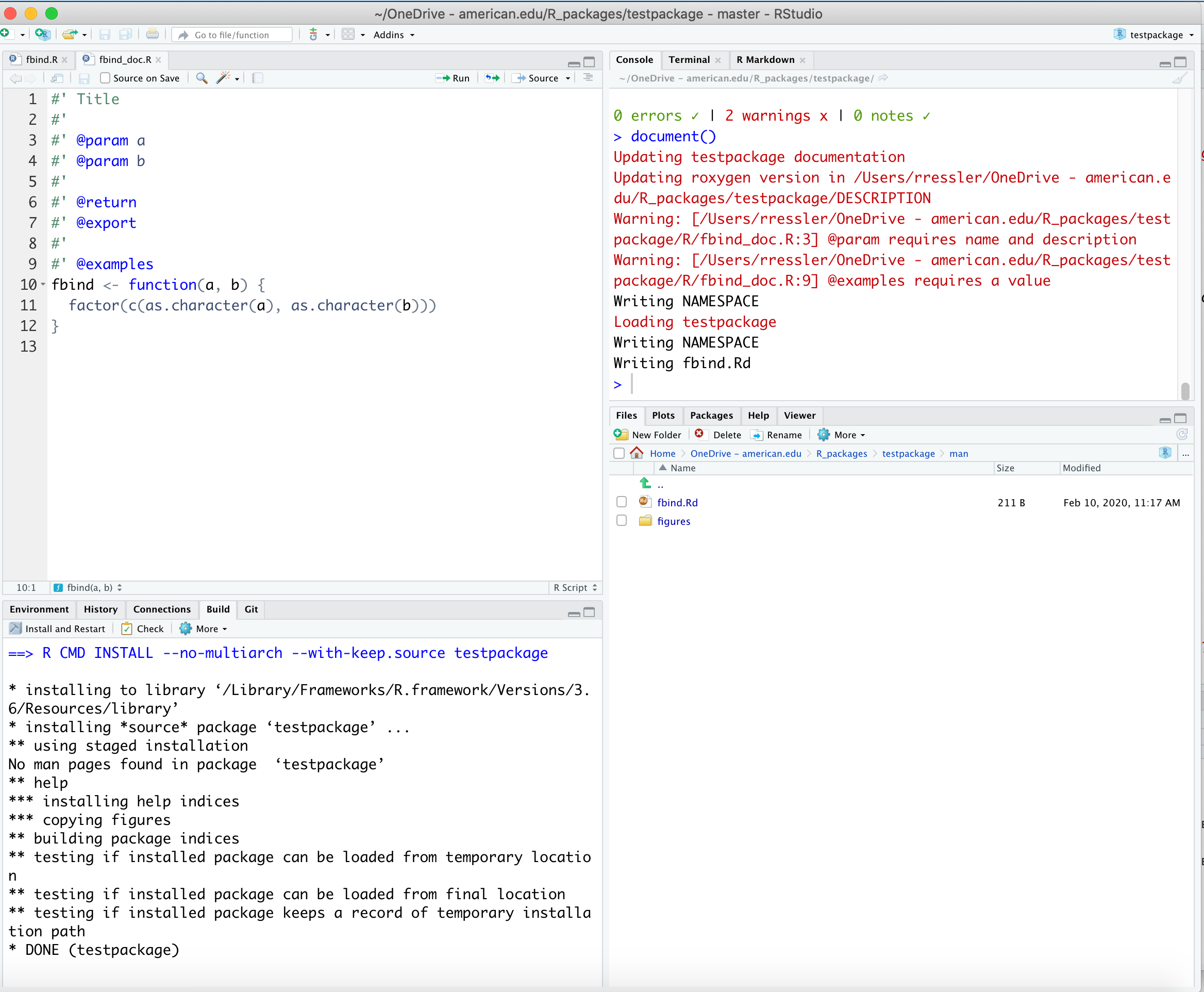
?function_name to preview your help file for each function.?fbind in the consoledocument() Also Updates the NAMESPACE fileIn addition to converting fbind()’s special comments into man/fbind.Rd, the call to document() updates the NAMESPACE file, based on any @export directives found in the Roxygen comments.
Execute: Open NAMESPACE for inspection.
wordlist()If you added the spelling package and it identifies words you know are spelled correctly you can use the function update_wordlist() to check spelling and add words to the wordlist.
The update_wordlist() function will prompt you about adding words (run after running check()).
Words you agree to add will be added to the packagename/inst/WORDLIST file in the package directory structure .
Execute: run update_wordlist()
create_package() to create a new packageuse_package() to add packages to the DESCRIPTION filefbind()document() to produce a help file and update the NAMESPACE filecheck() to see if the warnings went away.install() to install your locally developed package.library() to attach and use your package like any other package!NAMESPACE file as the function may not have been documented with the proper tags to update the NAMESPACE file with document().use_testthat(), use_test() and test()Once you have created your function and you think it is working, it is time to add some tests!
This is done using the use_test() function, and it works much the same way as use_r().
You tested fbind() informally, in a single example on the console. This is not repeatable and scalable.
Formalizing unit tests requires expressing a few concrete expectations about the correct fbind() result for various inputs.
First, declare your intent to write unit tests and to use the {testthat} package via use_testthat()
This initializes the unit testing machinery for your package.
Suggests: testthat to DESCRIPTION,tests/testthat/, andtest/testthat.R.Execute: Run use_testthat().
However, it’s still up to YOU to write the actual tests!
Execute: Open the fbind.R file for editing (the .R file you want to build test cases for must be open).
use_test("function_name") to create/open a test file stored under the tests/testthat folder.test-fbind.r to create two tests.
expect_identical().test-fbind.r file.fbind() gives an expected result when combining two factors and a character vector and a factor.library(testthat) in the console.load_all()test() (Hopefully you got a Woot!)test():browseVignettes(package = "dplyr") or browseVignettes(package = "rmarkdown")check().devtools::check() will attempt to knit it and ensure any data used in the vignette is documented and any packages used in the vignette are under the Imports ~ section of the DESCRIPTION file.packagename/inst/doc. That is no longer the case.VignetteEngine specified in the vignette YAML header to recreate the vignette when the package is installed.VignetteEngine will create a docfolder and then add three files for each vignette under the packagename/doc folder:
knitr.usethis::use_vignette("packagename")usethis::use_vignette("packagename") where packagename is the name of your package.vignettes/ directory.knitr to the Suggests and VignetteBuilder fields).vignettes/my-vignette.Rmd. ---
title: "Vignette Title"
output: rmarkdown::html_vignette
vignette: >
%\VignetteIndexEntry{Vignette Title}
%\VignetteEngine{knitr::rmarkdown}
\usepackage[utf8]{inputenc}
---Vignette: > entry contains a special block of metadata needed by R.\VignetteIndexEntry to provide the title of your vignette as you’d like it to appear in the vignette index.knitr to process the file, and the file is encoded in UTF-8 (the only encoding you should ever use to write vignettes).install.packages() from CRAN will have their vignettes recreated automatically and placed in the doc folder.devtools::install_github() or remotes::install_github() will not.build_vignettes = TRUE to have the vignettes recreated. If they are they will be in the doc folder.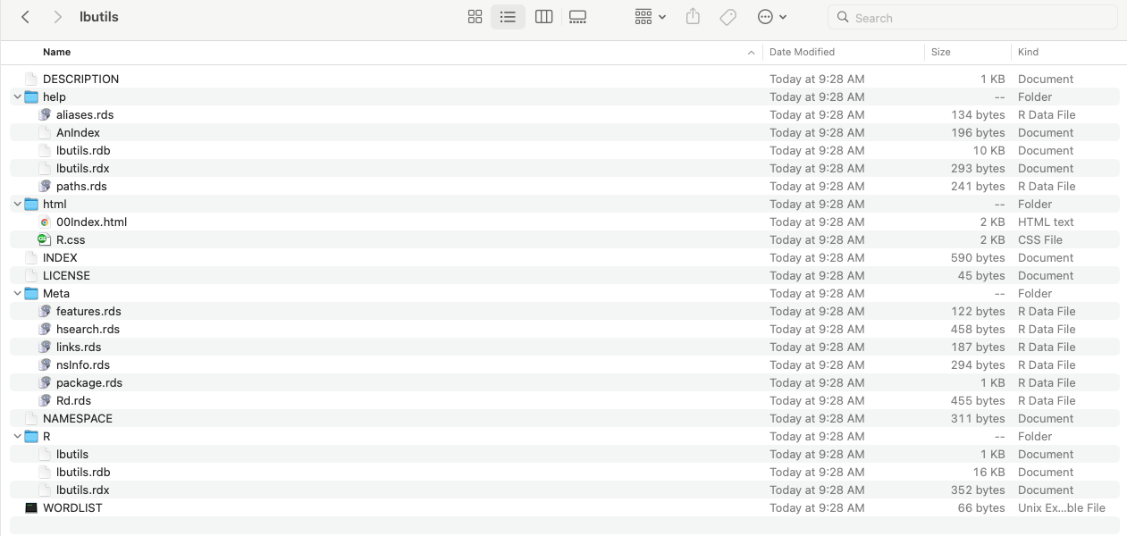
remotes::install_github("mygithubid/mypackagename", build_vignettes = TRUE) and it will look something like the following on the users computer.README file instructions.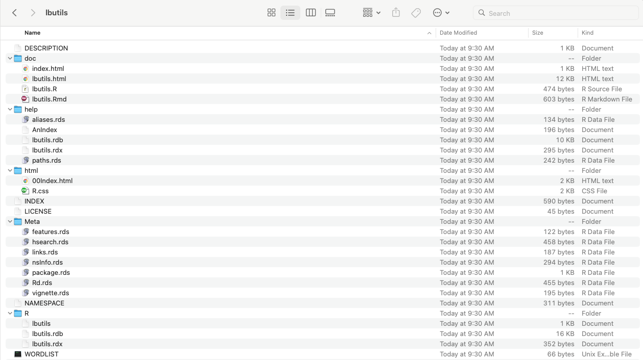
check(), it fails with an error about a missing package you know is installed.
DESCRIPTION (usually it should go in Suggests).devtools::install() instead.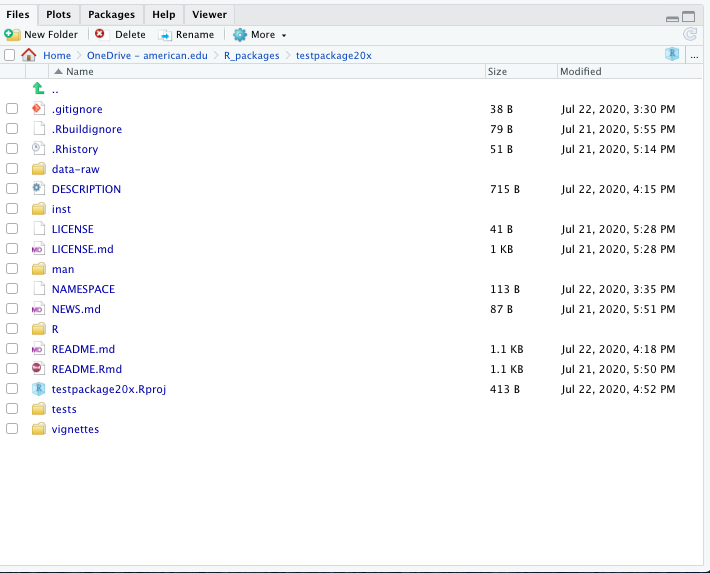
/Library/Frameworks/R.framework/Versions/Current/Resources/library
use_r("fcount") to open a new fileload_all() to simulate the installation of the package.fcount(iris$Species).document().install().use_github(organization = "my_organization", private = TRUE) will automatically create a private GitHub repo for your package at the GitHub organization you designate - assuming you have write privileges.organization = NULL will use your personal account.private = is FALSE so it will create it as a public repository.gh:"gh_token(). You should already have a Personal Authorization Token (PAT) from GitHub - see Creating a Personal Access Token
library(keyring) in the consolekey_set("GitHub_PAT") and enter the PAT when asked for the password.git remote add origin URL where you paste in the URL andgit push -u origin main.use_github(organisation = "XXX", private = TRUE) where XXX is the name of the other organization.git remote rm origin
use_github(organisation = "XXX", private = TRUE)Error: URL has a different value in DESCRIPTION.use_github_links(overwrite = TRUE) and it will update two URLS in your DESCRIPTION file to be the current remote location.git status and git remote -v.Many organizations enforce a style guide for writing as well as for any code.
Users accustomed to the Tidyverse coding style, like packages to be coded in accordance with the standards in the Tidyverse Style Guide Wickham (2021).
The style guide is intended to make all code easier to read, debug, and maintain by the original developer and especially by people other than the original developer.
There are two common packages for conducting static code analysis of your .R and .qmd/.RMD files: {lintr} and {styler}.
Both are available as RStudio Addins making it easy to keep your code properly formatted.
The {lintr} package Hester et al. (2024) has a default configuration for which items of “lint” to check.
The {styler} package Muller et al. (2024) can assist with checking and updating code in a .R file to correspond to the style guide.
install.packages("styler").use_tidy or go to usethis Helper functions Wickham et al. (2021).Completing the steps above should have allowed you to create a working package for sharing your code with yourself and with others.