17 Python in R
python, reticulate, numpy, pandas, matplotlib, seaborn
The code chunks for Python and R have different colors in this chapter.
- Code chunks for Python use this color.
- Code chunks for R use this color.
17.1 Introduction
17.1.1 Learning Outcomes
- Create strategies for integrating Python capabilities into an R workflow.
- Use Python in RStudio and R.
- Setup the RStudio environment for Python.
- Use the Python REPL in RStudio.
- Use Python Code Chunks and Python scripts in R.
- Recognize a Few Differences between Coding in R and Python.
- Employ basic Python and NumPy arrays.
- Read in and manipulate data with {Pandas}.
- Visualize data with {Matplotlib} and {Seaborn}.
17.1.2 References:
- matplotlib Users Guide Hunter et al. (2003)
- NumPy User Guide N. Developers (2023)
- pandas User Guide P. Developers (2023)
- {reticulate} package Ushey et al. (2023)
- {reticulate} vignette: Python Version Configuration Ushey et al. (2023)
- {reticulate} vignette: Installing Python Packages Ushey et al. (2023)
- {reticulate} vignette: Primer on Python for R Users Ushey et al. (2023)
- seaborn site Michael Waskom (2023)
- Using Python (in Quarto) Allaire et al. (2023)
17.1.2.1 Other References
- Another Book on Data Science: Learn R and Python in Parallel Zhang (2022)
- Getting started with Python using R and reticulate
- How to Use R and Python Together? Try These 2 Packages
- matplotlib Cheat Sheeets
- Python Data Science Handbook VanderPlas (2016)
- Python for Data Analysis McKinney (2022)
- Python Seaborn Plots in R using reticulate AbdulMajedRaja (2019)
- sklearn linear_model for LinearRegression Pedregosa et al. (2011)
17.1.3 Posit Philosophy on R and Python
R has its origins in being a high-level language that enables users to access capabilities in other languages, e.g., SQL, Spark, C++, bash, etc..
- R packages such as {dbplyr}, {sparklyR}, {shiny}, and {rcpp}, provide functions to enable users to choose the right capabilities for their task while hiding or wrapping the details of the other language.
- Non-scientific surveys show many data scientists use R and Python with a preference for using R for data visualization and statistical analysis and using Python for large scale data transformation and machine learning.
- It makes sense to enable R users to incorporate Python capabilities into their work and vice versa.
The {reticulate} package was developed by Posit (nee RStudio) to enable R users to incorporate python capabilities into their work.
- Starting with version 1.2 in 2018, RStudio Desktop has included features to make it easier to blend R and Python in the same project.
If you are working in a pure Python project, RStudio recommends using one of popular IDEs for Python, as they have more extensive support for a broad variety of python capabilities. These include:
Note, you can also run some R from inside python using the {rpy} package.
If working on a team with both R and python users, or combining R and Python in the same project, consider using Quarto instead of R Markdown.
- It allows different users to use RStudio or VS Code with Quarto Extension.
- See Quarto with VS Code.
17.1.4 Python Modules, Libraries, Packages, and Frameworks
Python uses a modular programming structure like R.
- Users can import a variety of packages or libraries to gain access to capabilities.
- However, the terms may be used slightly differently.
We’ll use the terms library and packages interchangeably, but to some there is a difference:
- A library is an umbrella term referring to a reusable chunk of code.
- Usually, a Python library contains a collection of related modules and packages.
- Actually, this term is often used interchangeably with “Python package” because packages can also contain modules and other packages (sub-packages).
- However, it is often assumed that while a package is a collection of modules, a library is a collection of packages.
- Using R as an example, the {tidyverse} package could be considered a “library” of packages while {ggplot2} could be considered a package focused on a specific set of capabilities.
- See Python Modules, Packages, Libraries, and Frameworks.
17.2 Setting Up Python for RStudio using the {reticulate} package
If you want to incorporate Python into an R workflow, the {reticulate} package provides a bridge between R and Python.
- As of reticulate 1.41+ (February 2025), the way reticulate manages Python has changed substantially.
With reticulate 1.41+, Python management now uses the new Python package manager {uv} Section A.6 to create a lightweight, isolated Python environment specifically for reticulate.
This means:
- {reticulate} no longer installs Miniconda by default.
- {reticulate} now creates a uv-managed virtual environment in a cache directory under your R user data.
- The environment is minimal and expecting you to declare dependencies for the packages needed for the project.
- This design reduces Python configuration issues on systems with multiple Python installations.
- Modern reticulate workflows rely on
py_require()orpy_install()to add packages as needed.
Because of these changes, always consult current reticulate documentation, not old tutorials or StackOverflow posts.
17.2.1 Configuring {reticulate} and Python
Use the Console to install the {reticulate} package with
install.packages("reticulate")’Library the {reticulate} package
- Identifying Python Dependencies
The {uv} workflow follows a “declare as needed” dependency model.
Use py_require() to declare the Python packages your project needs.
- Missing packages will be installed when Python is initialized.
For example, we can require the {numpy}, {pandas}, {matplotlib}, {seaborn}, {statsmodels} and {scikit-learn} packages.
Dependencies must be declared with py_require() before any Python code chunks or calls to import(), or py_config().
- Once Python initializes, the environment becomes “locked” and only
py_require("package", action = "add")is allowed.
- Run
py_discover_config()to inspect which Python reticulate would choose:
- You will typically see a path containing
.venvfile and a {uv}-style cache path such as:
python:         /Users/rressler/Courses/DATA-413-613/lectures_book/.venv/bin/python
libpython:      /Users/rressler/.local/share/uv/python/cpython-3.13.13-macos-aarch64-none/lib/libpython3.13.dylib
pythonhome:     /Users/rressler/Courses/DATA-413-613/lectures_book/.venv:/Users/rressler/Courses/DATA-413-613/lectures_book/.venv
virtualenv:     /Users/rressler/Courses/DATA-413-613/lectures_book/.venv/bin/activate_this.py
version:        3.13.13 (main, Apr  7 2026, 20:37:34) [Clang 22.1.1 ]
numpy:          /Users/rressler/Courses/DATA-413-613/lectures_book/.venv/lib/python3.13/site-packages/numpy
numpy_version:  2.4.4

NOTE: Python version was forced by VIRTUAL_ENV- This indicates {reticulate} will select its own isolated uv-based Python environment, which is expected.
- This does not create the environment, that happens later with
py_config(). - {reticulate} follows the rules outlined in Order of Discovery
- For removing old miniconda envs, use manual folder deletion or
reticulate::miniconda_remove().
- Once dependencies have been declared, run
py_config()to create and initialize the environment to be used by {reticulate}.
- If you want to use a different environment, see Providing hints.
python:         /Users/rressler/Courses/DATA-413-613/lectures_book/.venv/bin/python
libpython:      /Users/rressler/.local/share/uv/python/cpython-3.13.13-macos-aarch64-none/lib/libpython3.13.dylib
pythonhome:     /Users/rressler/Courses/DATA-413-613/lectures_book/.venv:/Users/rressler/Courses/DATA-413-613/lectures_book/.venv
virtualenv:     /Users/rressler/Courses/DATA-413-613/lectures_book/.venv/bin/activate_this.py
version:        3.13.13 (main, Apr  7 2026, 20:37:34) [Clang 22.1.1 ]
numpy:          /Users/rressler/Courses/DATA-413-613/lectures_book/.venv/lib/python3.13/site-packages/numpy
numpy_version:  2.4.4

NOTE: Python version was forced by VIRTUAL_ENV
This step:
- Creates the uv-managed environment (if not already created)
- Installs Python if required.
- Installs any missing packages declared via
py_require() - Finalizes (“locks”) the environment
After this step, only py_require(..., action = "add") is allowed to add new packages.
The combination ofpy_requires() and py_config() makes your project self-contained and portable across systems.
- To validate Python was installed and is available, run
reticulate::py_available().
- It should return
TRUE
- To see the list of installed packages use
py_list_packages().
- You may see only the packages listed in Step 3
- You may see many packages if they were previously installed for other projects in the same environment.
- To test everything is configured, run the following.
If the packages import without error, your {reticulate}-Python configuration is ready for use.
- {reticulate} manages its own internal Python, separate from Python used in VS Code, Jupyter, or {uv}-based projects.
- Do not modify the {reticulate} environment with pip, conda, or external tools.
Common issues:
Error: “After Python has initialized, only
action = 'add'with new packages is supported.”
→ Move yourpy_require()call into an early setup chunk and run it before any Python chunk,import(), orpy_config().ModuleNotFoundError
→ Declare the package withpy_require("packagename")in the setup chunk, then re-render.NameError: name 'sns' is not defined
→py_require("seaborn")installs seaborn, but you still need
import seaborn as snsinside the Python chunk.Works once, then fails later
→ Restart R and runquarto cleanin the terminal to remove cached Python sessions and outputs.Python confusion (wrong version or env)
→ reticulate 1.41+ manages its own uv environment; avoid pointing it at system Python or conda unless necessary.pip/conda not behaving as expected
→ Do not manage reticulate’s environment with pip/conda. Usepy_require()orpy_install()instead.
If the environment gets badly tangled, you can hard-reset it with:
and then re-run your setup chunk that calls py_require() and py_config().
17.3 Working with Python in RStudio
17.3.1 The Python REPL Shell
You are used to using the RStudio console as an interactive environment for working in R.
The console can also run an Interactive Python (IPython) shell.
To start an IPython shell run the following in the console:
This creates a Python “REPL” (“read–eval–print loop”) environment, which is an interactive programming environment.
- Note the triple
>>>prompt in Figure 17.1.
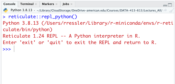
Exit the REPL by typing exit or quit.
17.3.2 Python Code Chunks
You can have Python chunks in quarto files by replacing the “r” at the beginning of the chunk by “python”.
You can access R objects in Python using the r object.
- That is,
r.xwill access, in Python, thexvariable defined using R.
You can access Python objects in R using the py object.
py$xwill access, in R, thexvariable defined using Python.
You can also begin a Python REPL by also hitting Control/Command + Enter inside the Python chunk (see Tools/Keyboard Shortcuts Help/Execute).
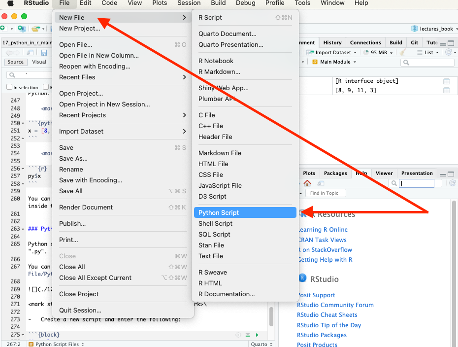
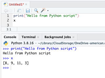
17.3.3 Python Script Files
Python scripts (where there is only Python code and no plain text) end in “.py”.
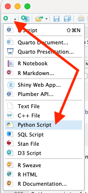
You can create a Python script in RStudio using the menu for File/New File/Python Script or the drop-down icon.
Create a new script and enter the following two lines:
print("Hello from Python script")
x
Use Run or Control/Command + Enter on each line of the Python script to start a Python REPL (if not already running) and execute the script in the console, as in Figure 17.4.
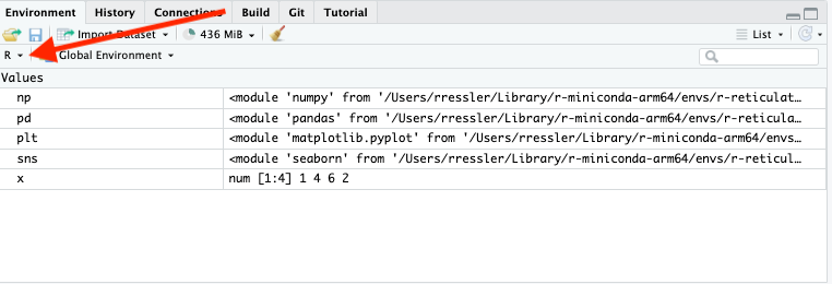
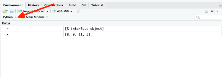
17.3.4 RStudio Environment Pane
You can switch the RStudio Environment from R to Python to see the different values in each environment.
- Objects in the Python environment also show their methods.
17.4 Differences between R and Python for the R user
17.4.1 White Space
White space matters in Python.
- In R, expressions are grouped into a code block with the curly braces operator
{ }.
In Python, expressions are grouped by making the expressions share an indentation level.
For example, an expression with an R code block might be:
if (TRUE) {This is one expression.This is another expression.}The equivalent in Python:
if True:|print("This is one expression.")|print("This is another expression.")
Python accepts tabs or spaces as the indentation spacer, but the rules get tricky when they’re mixed.
- Most style guides suggest, and IDEs default to, using only spaces.
17.4.2 Container Types
In R, the list() is a container you can use to organize R objects.
- There is no single direct equivalent in Python that supports all the same features.
Instead there are (at least) 4 different Python container types you will use:
- lists,
- dictionaries,
- tuples, and
- sets.
17.4.3 Lists
Python lists are typically created using bare brackets [ ].
- The Python built-in
list()function is more of a coercion function, closer in spirit to R’sas.list().
Python lists are modified in place, not copied and modified.
- Syntax for Python lists includes using
+and*with lists. - These are concatenation and replication operators, akin to R’s
c()andrep().
Indexing starts with 0 not 1.
17.4.4 Dictionaries
Dictionaries are most similar to R environments.
They are a container where you can retrieve items by name, though in Python the name (called a key in Python), does not need to be a string like in R.
- It can be any Python object with a
hash()method. - Note using
r_to_py()converts R named lists to python dictionaries.
17.4.5 Defining Functions with def
Python functions are defined with the def statement.
The syntax for specifying function arguments and default values is very similar to R.
The equivalent R snippet would be:
A Key Difference: Unlike R functions, the last value in a function is not automatically returned. Python requires an explicit return statement.
You can define Python functions that take a variable number of arguments, similar to ... in R.
- A notable difference is that R’s
...makes no distinction between named and unnamed arguments, but Python does. - In Python, prefixing with a single
*captures unnamed arguments, and two**signifies that keyword arguments are captured.
17.4.6 Defining Classes with class
One could argue that in R, the preeminent unit of composition for code is the function, and in Python, it’s the class.
- You can be a very productive R user and never explicitly use object-oriented constructs such as R6, reference classes, or similar R equivalents to the Python classes.
In Python however, understanding the basics of how class objects work is requisite knowledge, because classes are how you organize and find methods in Python.
- This is in contrast to R’s approach, where methods are found by dispatching from a generic function.
Like the def statement, the class statement binds an object to a new callable symbol, MyClass.
Python uses a strong naming convention, classes are typically CamelCase, and functions are typically snake_case.
After defining MyClass, you can interact with it, and see that it has type ‘type’.
Calling MyClass() creates a new object instance of the class, which has type ‘MyClass’.
Functions defined inside a class code block are called methods.
- Each time a method is called from a class instance, the instance is put into the function call as the first argument.
17.4.7 Integers and Floats
R users generally don’t need to be aware of the difference between integers and floating point numbers, but that’s not the case in Python.
- In R, writing a bare literal number like 12 produces a floating point type, whereas in Python, it produces an integer.
- You can produce an integer literal in R by appending an L, as in
12L.
Many Python functions expect integers, and will error when provided a float.
17.4.8 Sourcing Scripts
The source_python() function will source a Python script and make the objects it creates available within an R environment (by default the calling environment).
For example, use the RStudio File/New File/Python Script command to open a script file.
- Enter the following lines.
- Save it as
add.pyin apydirectory below your working directory.
Source it using the source_python() function (with a relative path).
Then you can run the python add() function directly from R or in an R code chunk:
17.4.9 Object Conversion
By default, when Python objects are returned to R they are converted to their equivalent R types.
However, if you’d rather make conversion from Python to R explicit, and work with native Python objects by default, you can pass convert = FALSE to the import function.
In this case, Python to R conversion will be disabled for the module returned from import.
For example:
- As illustrated above, if you need access to an R object at end of your computations, you can call the
py_to_r()function explicitly.
17.5 Numerical Python (NumPy)
| In R Use | In Python Use |
|---|---|
| Base R | numpy |
| dplyr/tidyr | pandas |
| ggplot2 | matplotlib/seaborn |
Create a Python script in RStudio or use python code chunks for the examples that follow.
17.5.1 Numpy Arrays
{NumPy} (short for Numerical Python) is the fundamental package or library for scientific computing in Python.
- {NumPy} is a Python library for working with arrays of data that enables efficient storage and data operations as the arrays grow larger.
{NumPy} provides a multidimensional array object, various derived objects (such as masked arrays and matrices), and an assortment of routines for fast operations on arrays.
- These include: mathematical, logical, shape manipulation, sorting, selecting, I/O, discrete Fourier transforms, basic linear algebra, basic statistical operations, random simulation and much more.
Let’s import the {numpy} package:
When importing a python package, we can create a nickname (alias) for it.
They are shorter than the package name to allow for less typing.
Use
import my_package as my_nickname.
Many packages have “standard” nicknames and you should avoid using the nicknames for other objects even if not importing the package.
The standard nickname for {numpy} is np.
In Python, assign variables with =, not <-.
The arithmetic operations (+, -, *, /) are the same.
Comments also begin with a #.
Help files are called the same way.
Python lists are like R lists in that they can have the different types.
You create Python lists with brackets [ ].
NumPy Arrays (class ndarray) are the Python equivalent to R atomic vectors (where each element must be the same type) but may have multiple dimensions.
- You use the
array()method of the {numpy} package to create a numpy array (you give it a list as input). - When calling a method from a package, you have to fully specify the package name and method using the syntax
package.method()
You can do vectorized operations on NumPy arrays.
Two vectors of the same size (length) can be added/subtracted/multiplied/divided.
Vector Recycling vs. Broadcasting
R and Python take fundamentally different approaches to operations on vectors (arrays) of unequal length.
R: Vector Recycling
R silently recycles shorter vectors to match the length of longer ones:
c(1, 2, 3, 4) + c(10, 20) #> 11 22 13 24
- The shorter vector is repeated (10, 20, 10, 20).
- If lengths are not multiples, R still recycles but produces a warning.
- The shorter vector is repeated (10, 20, 10, 20).
NumPy (Python): Broadcasting
NumPy does not recycle vectors. Instead, it applies broadcasting, where array shapes must be compatible:
- Two dimensions are compatible if they are equal, or if one dimension is
1. - If shapes cannot be aligned, NumPy raises an error.
- Two dimensions are compatible if they are equal, or if one dimension is
Example:
import numpy as np np.array([1, 2, 3, 4]) + np.array([10, 20]) # ValueError: operands could not be broadcast together
Broadcasting is powerful for multi-dimensional operations but never silently repeats arrays the way R does.
You extract or subset individual elements of an array just like in R, using brackets [].
Indexing of numpy ndarrays is different from R in that the numpy slicing syntax x:y selects from element x up to y-1. See Indexing on ndarrays
You can extract arbitrary (non-contiguous) elements by subsetting with an index array.
Key Difference: Python starts counting from 0, not 1.
- So the first element of a vector is
vec[0], notvec[1]. - You can still use negative indices for indexing from the end of the array.
Combine two arrays via np.concatenate() (note the use of brackets here inside the ([]) to create a list).
17.5.2 Useful Functions for Operating on Vectors
In R, functions operate on objects (e.g. log(x), sort(x), etc.).
Python also has functions that operate on objects.
- But, objects usually have functions that are directly associated with them.
- These functions are called “methods”.
You access these functions by fully specifying the object and method with the syntax object.function(), i.e., a period between the object name and the function name.
- You can use tab completion to scroll through the available methods of an object.
- Recall that the object is placed as the first argument in the class method.
Start a REPL with reticulate::repl_python() (if not running) and enter ?vec.sort in the REPL console.
There are many other useful np.* functions that operate on objects.
Missing Values: NA in R vs. NaN in NumPy
R: NA
- Represents missing or undefined values.
NA == NAis alwaysNA(unknown).- Functions such as
match(),duplicated(), and joins treatNAas a special placeholder.
NumPy: NaN
NumPy follows IEEE floating-point semantics:
NaN != NaNis always true.NaNnever compares equal to anything (including itself).- Matching-like operations (
==,in1d,unique, joins) therefore never match NaNs.
Example:
a = np.array([1, np.nan, 3]) b = np.array([np.nan]) a == b # array([False, False, False])
To treat missing values as matching, you must explicitly detect them using
np.isnan().
Treatment of Missing Values in Math Functions (mean, max, etc.)
R Behavior
Most math functions (e.g.,
mean(),sum(),max()) returnNAif the input contains anyNAvalues, unless the user explicitly removes them:mean(c(1, 2, NA)) #> NA
mean(c(1, 2, NA), na.rm = TRUE) #> 1.5
NumPy Behavior
NumPy math functions behave differently:
Standard functions (
np.mean,np.max,np.sum) return NaN if any NaN is present.“nan-safe” variants (
np.nanmean,np.nanmax,np.nansum) ignore NaNs, similar tona.rm = TRUEin R.Example:
x = np.array([1, 2, np.nan])
np.mean(x) # nan
np.nanmean(x) # 1.5
NumPy therefore forces the user to choose between:
- strict NaN propagation (
np.mean,np.max, etc.) - ignoring NaNs (
np.nanmean,np.nanmax, etc.)
- strict NaN propagation (
17.5.3 Booleans (Python’s logicals)
Python uses True and False. It uses the same comparison operators as R.
- These are also vectorized.
The logical operators have a Key Difference: “Not” uses a different character, the tilde ~.
&And|Or~Not
You subset a vector using Booleans inside the [ ] as you would in R.
When you are dealing with single logicals, instead of arrays of logicals, use and, or, and not instead.
17.5.3.1 Exercise:
- Consider two vectors.
\[ y = (1, 7, 1, 2, 8, 2)\\ x = (4, 6, 2, 7, 8, 2) \]
Calculate their inner product.
\[y_1x_1 + y_2x_2 + y_3x_3 + y_4x_4 + y_5x_5 + y_6x_6\]
Do this using vectorized operations.
17.5.3.2 Exercise
Provide two ways of extracting the 2nd and 5th elements of this vector.
17.5.3.3 Exercise:
Extract all elements from the previous vector between 5 and 8 (inclusive). Use predicates.
17.5.4 Multi-Dimensional Arrays
NumPy can also support multi-dimensional arrays.
Each array has attributes ndim (the number of dimensions), shape (the size of each dimension), and size (the total size of the array).
In a multi-dimensional array, items can be accessed using a comma-separated tuple of indices.
Values can also be modified using any of the above index notation.
Key Difference: NumPy arrays have a fixed type.
- This means if you attempt to insert a floating-point value into an integer array, the value will be silently truncated.
NumPy has capabilities to reshape and index multi-dimensional arrays.
17.5.5 Heterogeneous Data
NumPy uses “structured arrays” and “record arrays” to provide efficient storage for compound, heterogeneous data.
- They could be considered conceptually similar to R list vectors in that all elements do not have to be of the same type.
17.6 Data Manipulation with Pandas
- This section is based primarily on work by Professor David Gerard.
17.6.1 Intro to Pandas
{Pandas} is a newer package built on top of {NumPy}, and provides an efficient implementation of a data frame.
Python DataFrames are essentially multi-dimensional arrays with attached row and column labels, and often with heterogeneous types and/or missing data.
- {Pandas} objects can be thought of as enhanced versions of {NumPy} structured arrays in which the rows and columns are identified with labels rather than simple integer indices.
Import both {NumPy} and {Pandas} into the Python environment.
A Pandas Series is a one-dimensional array of indexed data.
- It can be created from a list or array as follows and we can see the values using the
object.valuessyntax.
The essential difference with a Numpy array is the Pandas Series has an explicitly defined index associated with the values instead of an implicit index.
- Note, the index need not be an integer, but can consist of values of any desired type.
- For example, if we wish, we can use strings as an index for the series.
If a Series is an analog of a one-dimensional array with flexible indices, a “Data Frame” is an analog of a two-dimensional array with both flexible row indices and flexible column names.
Think of a Data Frame as a sequence of aligned Series objects.
Here, by “aligned” we mean they share the same index.
17.6.2 Pandas versus Tidyverse
Keep these equivalencies in mind:
<Series>.fun()meansfun()is a method of the<Series>object. -<DataFrame>.fun()meansfun()is a method of the<DataFrame>object.tidyverse pandas arrange()<DataFrame>.sort_values()bind_rows()pandas.concat()filter()<DataFrame>.query()pivot_longer()<DataFrame>.melt()glimpse()<DataFrame>.info()and<DataFrame>.head()group_by()<DataFrame>.groupby()if_else()numpy.where()left_join()pandas.merge()library()importmutate()<DataFrame>.eval()and<DataFrame>.assign()read_csv()pandas.read_csv()recode()<DataFrame>.replace()rename()<DataFrame>.rename()select()<DataFrame>.filter()and<DataFrame>.drop()separate()<Series>.str.split()slice()<DataFrame>.iloc()pivot_wider()<DataFrame>.pivot_table().reset_index()summarize()<DataFrame>.agg()unite()<Series>.str.cat()|>, or %>%| Enclose pipeline in()`
17.6.3 Importing Libraries
Python: import <package> as <alias>.
Use the alias (nickname) you define during the import in place of the package name.
- R equivalent
17.6.4 Reading in and Printing Data
Pandas has a family of functions for reading in data from fixed-width files.
Use tab-completion to scroll through them.
We’ll demonstrate most methods with the “estate” data we’ve seen before.
You can read about these data here: https://github.com/AU-datascience/data/blob/main/413-613/data_estate.qmd
Python: pd.read_csv().
R equivalent:
Use the info() and head() methods to see the data.
<class 'pandas.DataFrame'>
RangeIndex: 522 entries, 0 to 521
Data columns (total 12 columns):
 #   Column   Non-Null Count  Dtype
---  ------   --------------  -----
 0   Price    522 non-null    int64
 1   Area     522 non-null    int64
 2   Bed      522 non-null    int64
 3   Bath     522 non-null    int64
 4   AC       522 non-null    int64
 5   Garage   522 non-null    int64
 6   Pool     522 non-null    int64
 7   Year     522 non-null    int64
 8   Quality  522 non-null    str
 9   Style    522 non-null    int64
 10  Lot      522 non-null    int64
 11  Highway  522 non-null    int64
dtypes: int64(11), str(1)
memory usage: 51.5 KB Price Area Bed Bath AC ... Year Quality Style Lot Highway
0 360000 3032 4 4 1 ... 1972 Medium 1 22221 0
1 340000 2058 4 2 1 ... 1976 Medium 1 22912 0
2 250000 1780 4 3 1 ... 1980 Medium 1 21345 0
3 205500 1638 4 2 1 ... 1963 Medium 1 17342 0
4 275500 2196 4 3 1 ... 1968 Medium 7 21786 0
[5 rows x 12 columns]R equivalent:
# A tibble: 6 × 12
   Price  Area   Bed  Bath    AC Garage  Pool  Year Quality Style   Lot Highway
   <dbl> <dbl> <dbl> <dbl> <dbl>  <dbl> <dbl> <dbl> <chr>   <dbl> <dbl>   <dbl>
1 360000  3032     4     4     1      2     0  1972 Medium      1 22221       0
2 340000  2058     4     2     1      2     0  1976 Medium      1 22912       0
3 250000  1780     4     3     1      2     0  1980 Medium      1 21345       0
4 205500  1638     4     2     1      2     0  1963 Medium      1 17342       0
5 275500  2196     4     3     1      2     0  1968 Medium      7 21786       0
6 248000  1966     4     3     1      5     1  1972 Medium      1 18902       0
Rows: 522
Columns: 12
$ Price   <dbl> 360000, 340000, 250000, 205500, 275500, 248000, 229900, 150000…
$ Area    <dbl> 3032, 2058, 1780, 1638, 2196, 1966, 2216, 1597, 1622, 1976, 28…
$ Bed     <dbl> 4, 4, 4, 4, 4, 4, 3, 2, 3, 3, 7, 3, 5, 5, 3, 5, 2, 3, 4, 3, 4,…
$ Bath    <dbl> 4, 2, 3, 2, 3, 3, 2, 1, 2, 3, 5, 4, 4, 4, 3, 5, 2, 4, 3, 3, 3,…
$ AC      <dbl> 1, 1, 1, 1, 1, 1, 1, 1, 1, 0, 0, 1, 1, 1, 1, 1, 1, 1, 1, 1, 1,…
$ Garage  <dbl> 2, 2, 2, 2, 2, 5, 2, 1, 2, 1, 2, 3, 3, 2, 2, 2, 2, 2, 2, 2, 2,…
$ Pool    <dbl> 0, 0, 0, 0, 0, 1, 0, 0, 0, 0, 1, 0, 0, 0, 0, 0, 0, 0, 0, 0, 0,…
$ Year    <dbl> 1972, 1976, 1980, 1963, 1968, 1972, 1972, 1955, 1975, 1918, 19…
$ Quality <chr> "Medium", "Medium", "Medium", "Medium", "Medium", "Medium", "M…
$ Style   <dbl> 1, 1, 1, 1, 7, 1, 7, 1, 1, 1, 7, 1, 7, 5, 1, 6, 1, 7, 7, 1, 2,…
$ Lot     <dbl> 22221, 22912, 21345, 17342, 21786, 18902, 18639, 22112, 14321,…
$ Highway <dbl> 0, 0, 0, 0, 0, 0, 0, 0, 0, 0, 0, 0, 0, 0, 0, 0, 0, 0, 0, 0, 0,…
17.6.5 DataFrames and Series
Pandas reads in tabular data as a DataFrame object.
- Just as R’s
data.frameis a list of atomic vectors with the same length, panda’sDataFramecontains a list ofSeriesobjects. - A
Seriesobject is a generalization of a numpy array. So you can use {numpy} functions on it.
17.6.6 Extract Variables
Python: Use a where period to extract variables, e.g., dataframe.variable.
This extracts the column as a {Pandas} series.
Then you can use all of those {numpy} functions on the series.
R equivalent: Use a $.
17.6.7 Filtering/Arranging Rows (Observations)
Filter rows based on booleans (logicals) with query().
- The queries need to be in quotes.
- Some people use bracket notation, which is more similar to base R
R equivalent:
Select rows by numerical indices with iloc().
R equivalent:
Arrange rows by sort_values().
R equivalent
17.6.7.1 Exercise:
Use {pandas} and then {tidyverse} to extract all medium quality homes that have a pool and arrange the rows in increasing order of price.
Note the use of the period . to “pipe” to subsequent methods.
17.6.8 Selecting Columns (Variables)
Column variables are selected using filter() whereas in R, filter() subsets rows.
Some people use bracket notation, which is more similar to Base R.
- The inner brackets
[ ]create a Python list which is then used by the outer brackets[ ]for sub-setting the columns.
R equivalent:
Dropping a column is done by drop().
- The
axis = 1argument says to drop by columns (rather than by “index”, which is something we haven’t covered).
R: Use select() with a minus sign.
Renaming variables is done with rename().
R equivalent.
# A tibble: 522 × 12
    price  area   Bed  Bath    AC Garage  Pool  Year Quality Style   Lot Highway
    <dbl> <dbl> <dbl> <dbl> <dbl>  <dbl> <dbl> <dbl> <chr>   <dbl> <dbl>   <dbl>
 1 360000  3032     4     4     1      2     0  1972 Medium      1 22221       0
 2 340000  2058     4     2     1      2     0  1976 Medium      1 22912       0
 3 250000  1780     4     3     1      2     0  1980 Medium      1 21345       0
 4 205500  1638     4     2     1      2     0  1963 Medium      1 17342       0
 5 275500  2196     4     3     1      2     0  1968 Medium      7 21786       0
 6 248000  1966     4     3     1      5     1  1972 Medium      1 18902       0
 7 229900  2216     3     2     1      2     0  1972 Medium      7 18639       0
 8 150000  1597     2     1     1      1     0  1955 Medium      1 22112       0
 9 195000  1622     3     2     1      2     0  1975 Low         1 14321       0
10 160000  1976     3     3     0      1     0  1918 Low         1 32358       0
# ℹ 512 more rows
17.6.8.1 Exercise:
- Use {pandas} and then {tidyverse} to select
Year,Price, andArea.
17.6.9 Creating New Variables (Mutate)
New variables are created in Python using eval().
- Place the entire expression in quotes (not tick marks).
You can also use assign(), but then you need to reference the DataFrame as you extract variables.
R equivalent:
17.6.9.1 Exercise:
Use {pandas} and then {tidyverse} to create a new variable, ppa with the calculated price per unit area.
17.6.10 Piping
All of these pandas functions return a DataFrame so we can apply methods to the DataFrame by just appending methods to the end.
Suppose we want to find the total number of beds and baths, and select the price and this total number.
Try the following code.
- If you want to place these operations on different lines, then just place the whole operation within parentheses similar to using
{}in R for an expression.
This looks similar to piping in R.
17.6.10.1 Exercise:
Use {pandas} with piping to extract all medium quality homes that have a pool and arrange the rows in increasing order of price.
17.6.11 Summaries and Grouped Summaries
Summaries can be calculated using the DataFrame’s agg() method.
- You usually first select the columns whose summaries you want before running
agg().
R equivalent
Use the DataFrame’s groupby() method to create group summaries.
R equivalent
You can get multiple summaries by passing a list of functions (created using [ ]).
You can create your own functions (with dev()) and pass those.
17.6.12 Recoding Variable Values
Use replace() with a dict object to recode variable values.
- Useful with Categorical variables, the equivalent to R Factors.
R equivalent:
To recode values based on logical conditions, use np.where().
R equivalent.
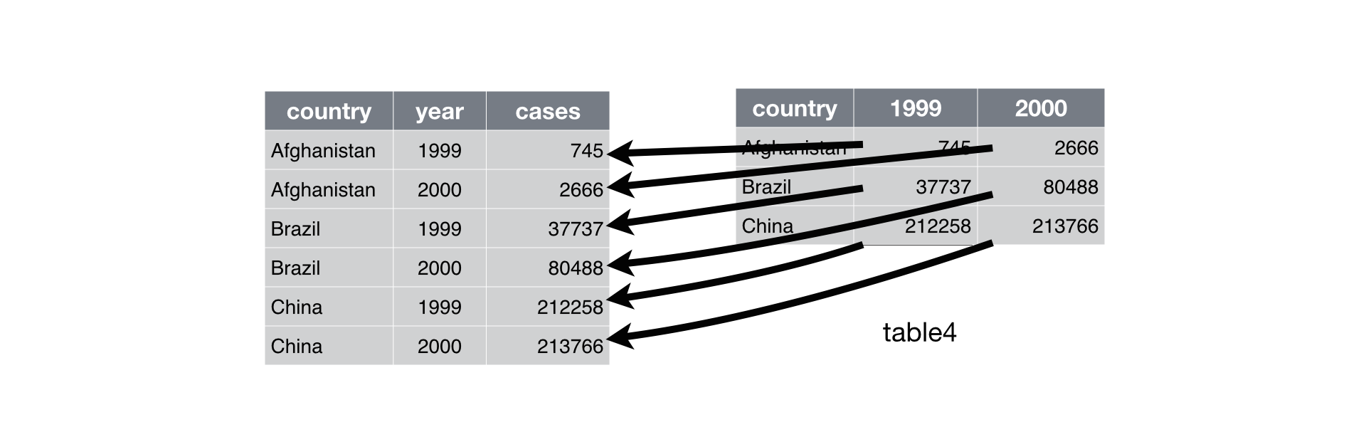
17.6.13 Reshape DataFrames Longer with Melt
Problem: One variable spread across multiple columns.
- Column names are actually values of a variable.
- Recall
table4afrom the {tidyr} package.
Solution: melt() (similar to {data.table}).
R equivalent.
- R4DS visualization:
17.6.13.1 Exercise:
Use {pandas} to reshape the monkeymem data frame (available at https://raw.githubusercontent.com/AU-datascience/data/main/413-613/estate.csv.
- The cell values represent identification accuracy of some objects (in percent of 20 trials).
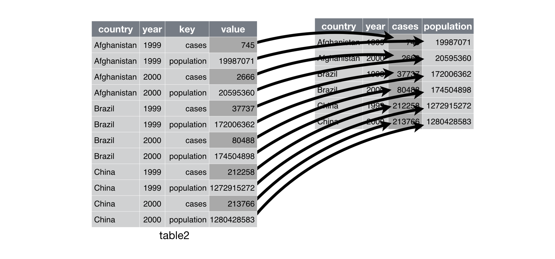
17.6.14 Reshape Dataframes Wider with pivot_table()
Problem: One observation is spread across multiple rows.
- One column contains variable names. One column contains values for the different variables.
- Recall
table2from the {tidyr} package. - Load and assign to a python variable.
Solution: pivot_table() followed by reset_index().
pivot_table()creates a table with anindexattribute defined by the columns you pass to theindexargument.- The
reset_index()converts that attribute to columns and changes theindexattribute to a sequence[0, 1, ..., n-1].
R equivalent.
- R4DS visualization:
17.6.14.1 Exercise:
Use {pandas} to read and reshape the flowers1 dataframe (available at https://raw.githubusercontent.com/AU-datascience/data/main/413-613/flowers1.csv).
17.6.15 Separating a Variable into Two or more Columns
Sometimes we want to split a column based on a delimiter.
Use object.column.str.split(pat = "", expand = True)
R equivalent.
17.6.15.1 Exercise:
- Use {pandas} to read and separate the
flowers2data frame (available at https://raw.githubusercontent.com/AU-datascience/data/main/413-613/flowers2.csv).
Show code
```{python}
#| eval: false
#| code-fold: true
flowers2 = pd.read_csv("https://raw.githubusercontent.com/AU-datascience/data/main/413-613/flowers2.csv", sep=";")

flowers2[['Flowers', 'Intensity']] = flowers2['Flowers/Intensity'].str.split(pat = "/", expand = True)

flowers2 = flowers2.drop('Flowers/Intensity', axis = 1)
```
17.6.16 Uniting Variables
Sometimes we want to combine two columns of character/string variables into one column.
Use str.cat() to combine two columns century and year.
R equivalent.
17.6.16.1 Exercise:
- Use {pandas} to re-unite the data frame you separated from the
flowers2exercise. - Use a comma for the separator.
17.6.17 Combining and Joining Two DataFrames
We will use these DataFrames for the examples below.
Binding rows is done with pd.concat().
R equivalent.
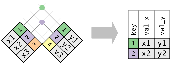
All joins use pd.merge().
Inner Join (visualization from R4DS).
Outer Joins (visualization from RDS):
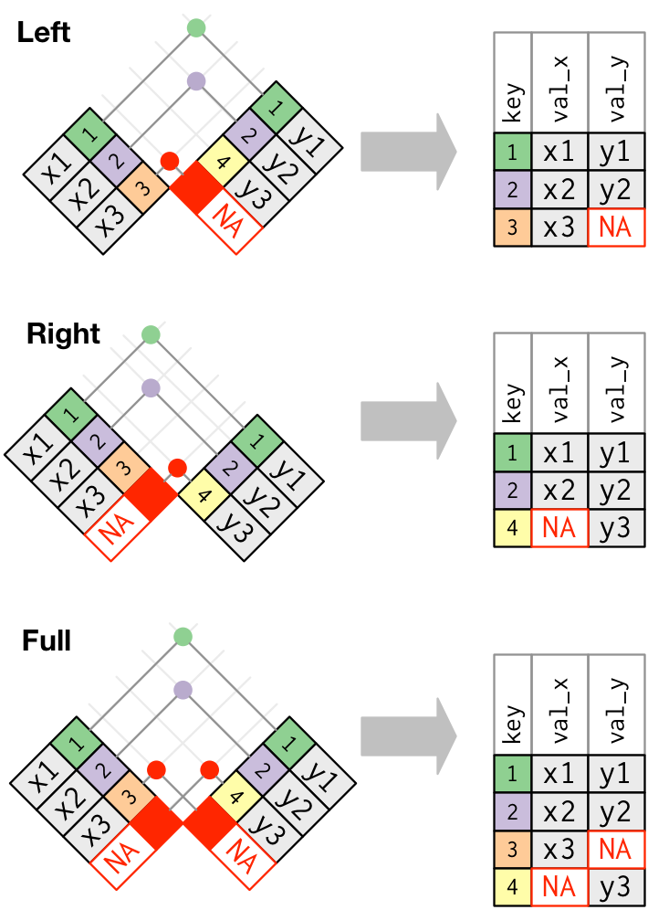
Left Join
Right Join
Full Join (try not to use very often …)
- Use the
left_onandright_onarguments if the keys are named differently. - The
onargument can take a list of key names if your key is multiple columns.
17.7 Python Matplotlib and Seaborn Libraries
- This section is based primarily on work by Professor David Gerard.
{Matplotlib} is a comprehensive library for creating static, animated, and interactive visualizations in Python.
- {Matplotlib} graphs your data onto Figures (e.g., windows, Jupyter widgets, etc.), each of which can contain one or more axes.
{Seaborn} is a library for making statistical graphics in Python.
- It builds on top of {matplotlib} and integrates closely with {pandas} Series and DataFrames.
- It lets you focus on what the different elements of your plots mean, rather than on the details of how to draw them.
Seaborn has different modules of functions for different analytic purposes, e.g., “relational”, “distributional”, and “categorical” modules.
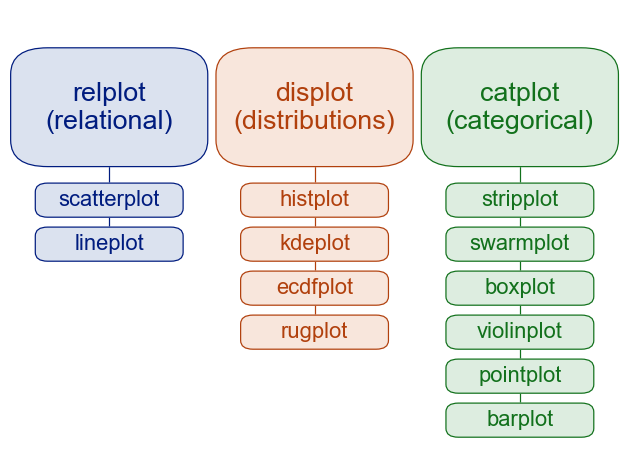
Seaborn has extensive documentation, a tutorial as well as a gallery of examples.
Let’s load {reticulate} and {ggplot2} in R and load the mpg data set.
All other code in this section will be Python unless otherwise marked.
Import matplotlib.pyplot and {seaborn} in python and create a python data frame from mpg.
17.7.1 Create, Show, and Clear plots.
Use a plotting function to create a plot object.
- Matplotlib will return information about the plot unless you assign a name to it.
- Use
.set(title='My Title')to add a title.
Use plt.show() to display a plot that has been created.
Use plt.close() to close the plot and free memory.
- Use
plt.clf()to clear a plot before making a new plot on the same layout.
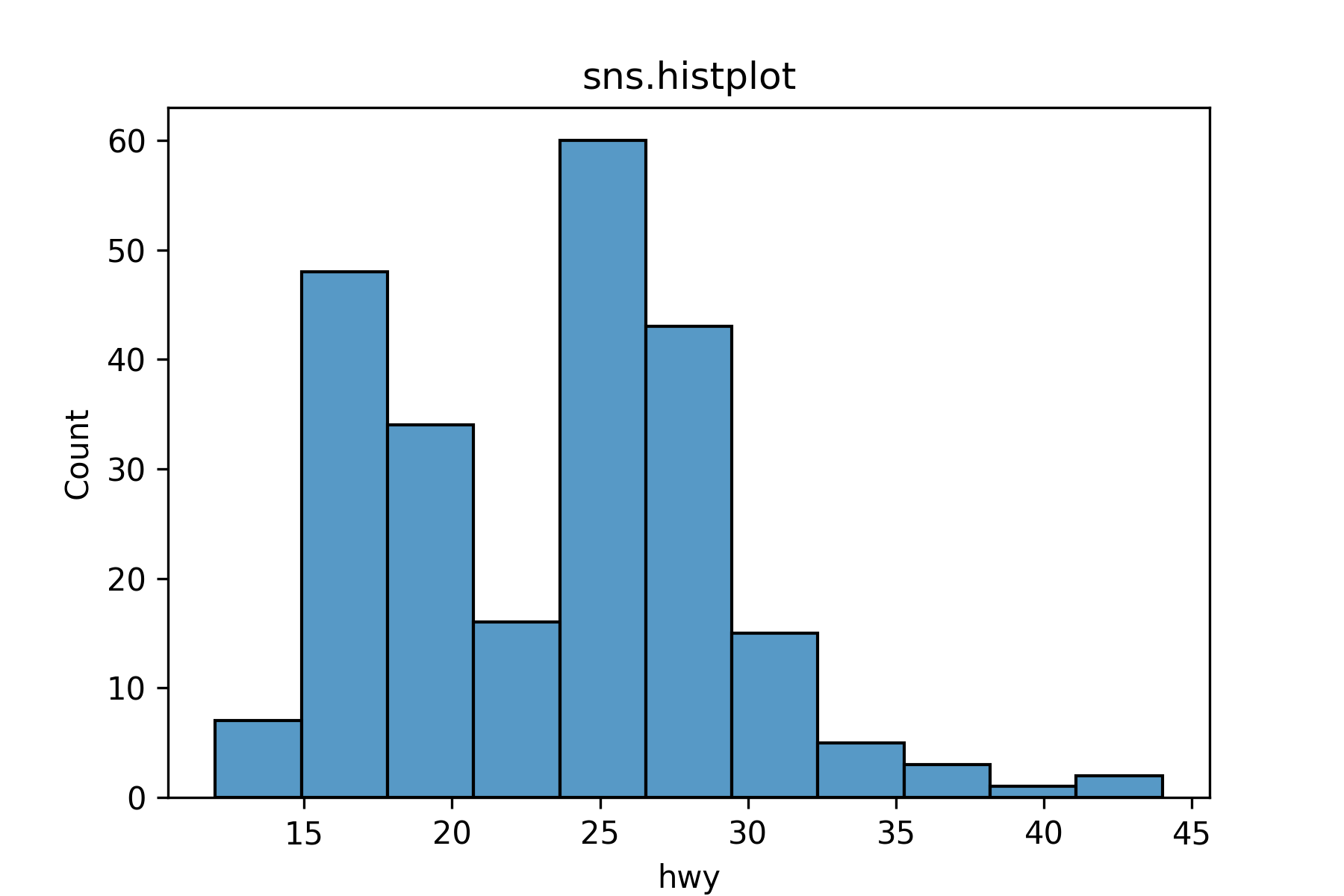
17.7.2 One Quantitative Variable: Histogram
sns.histplot() makes a histogram.
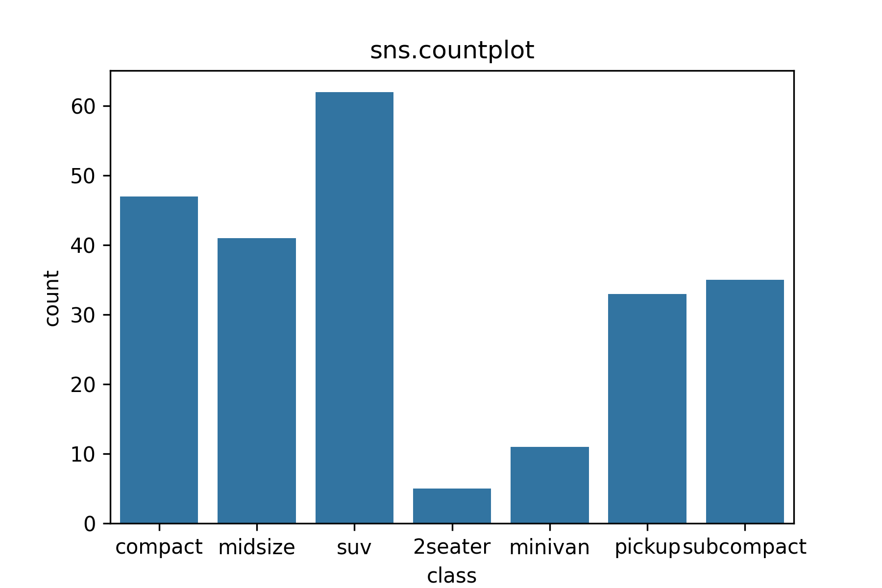
17.7.3 One Categorical Variable: Barplot
Use sns.countplot() to make a barplot of the distribution of a categorical variable.
17.7.4 One Quantitative Variable, One Categorical Variable: Boxplot
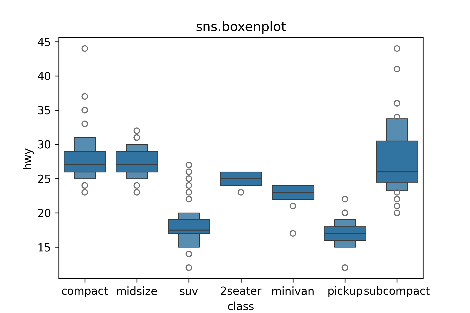
Use sns.boxplot() to make boxplots.
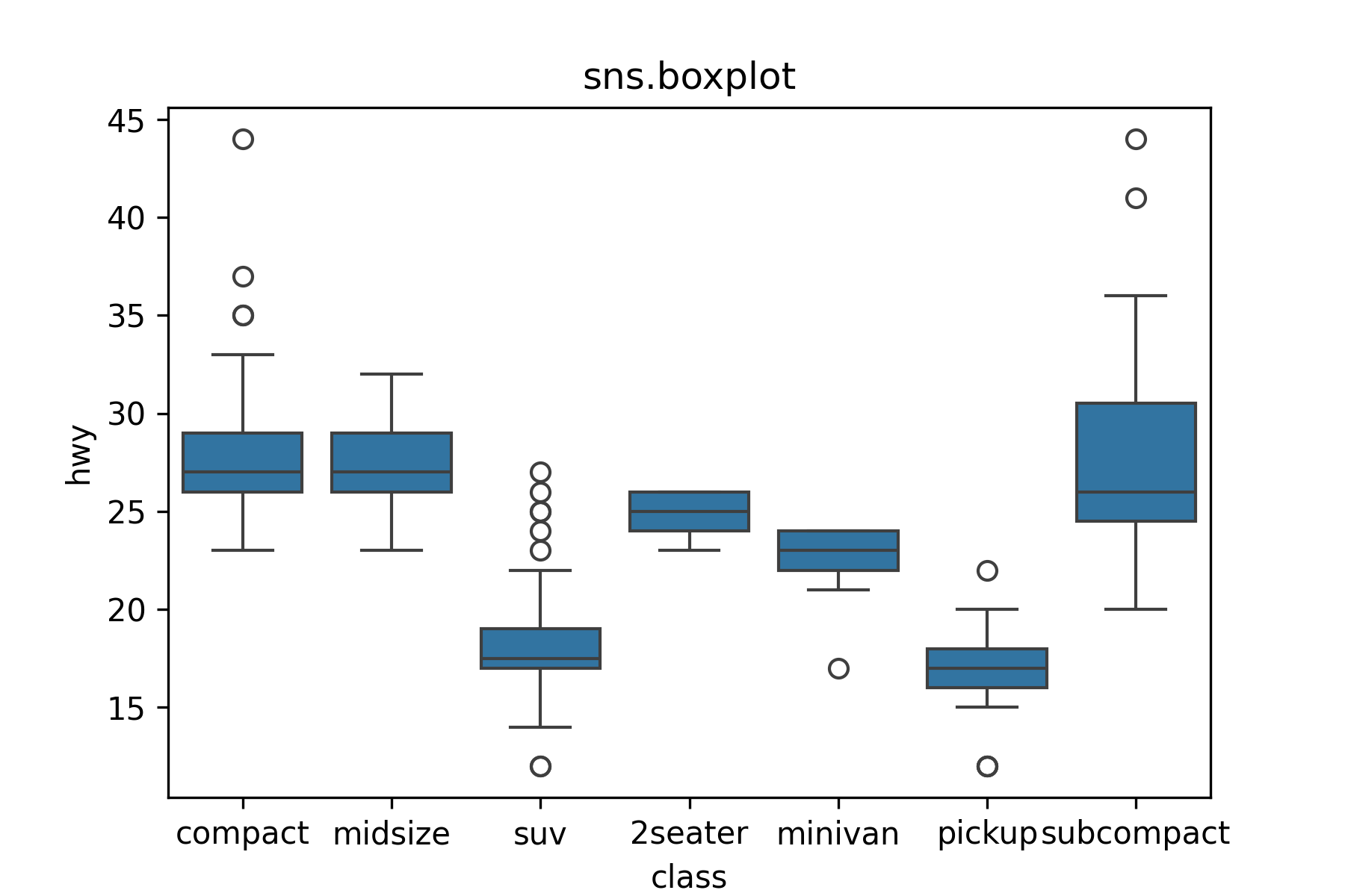
A boxenplot is a cool graphic that gives you more quantiles.
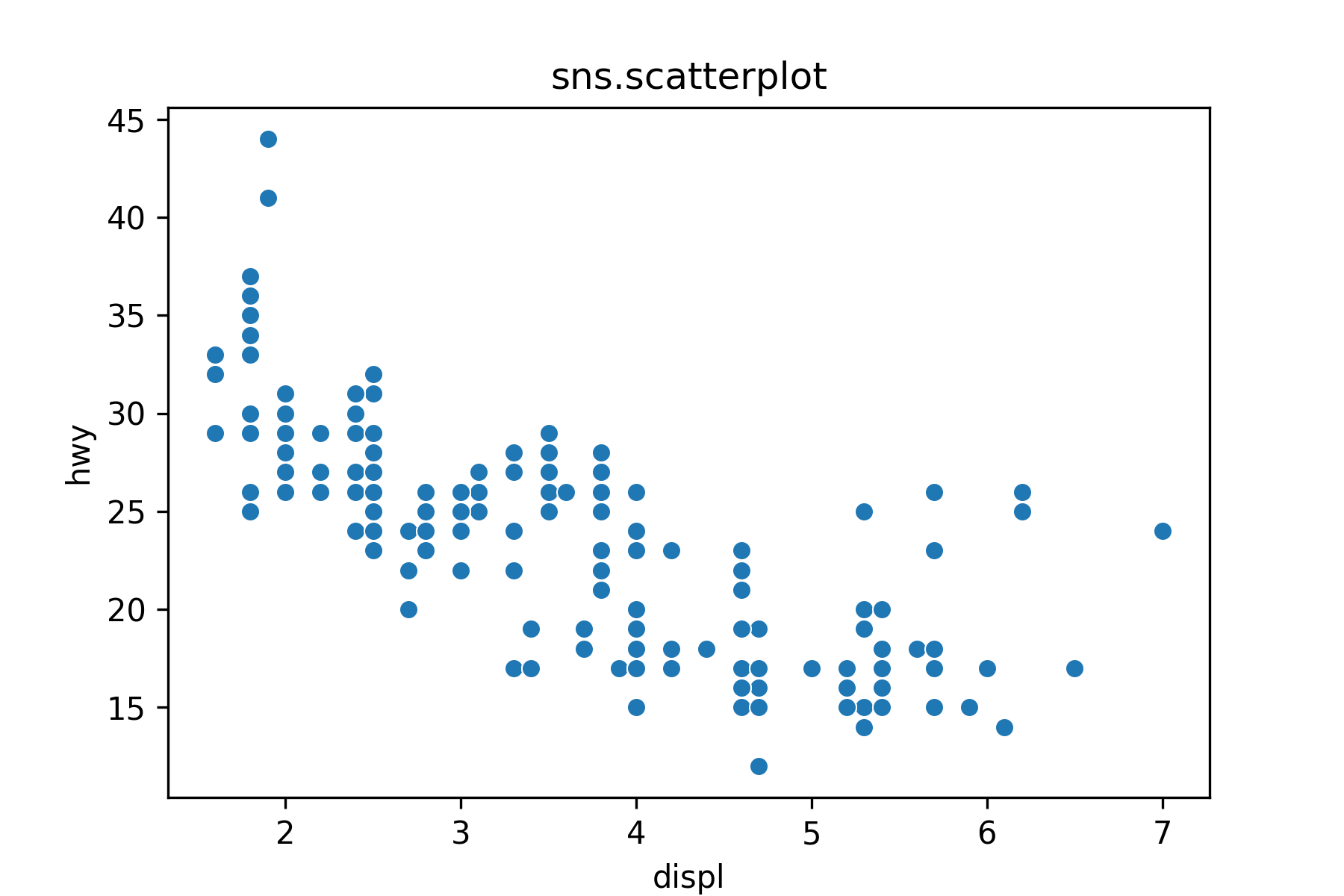
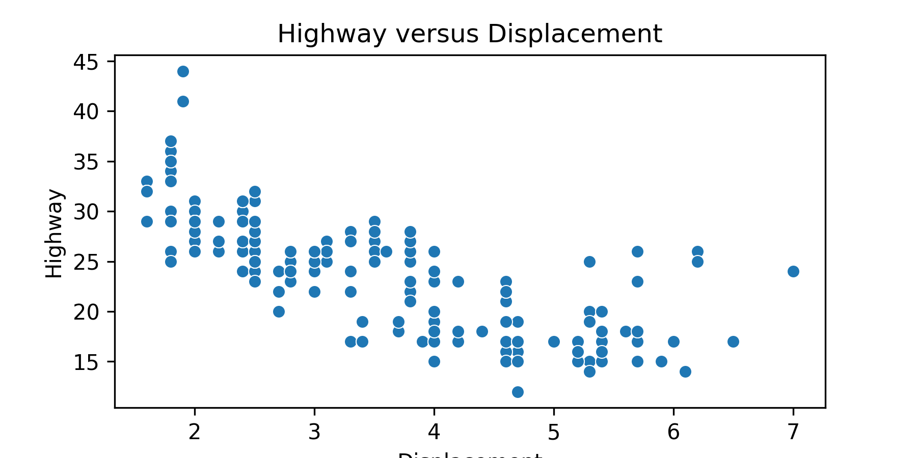
17.7.5 Two Quantitative Variables: Scatterplot
Use sns.scatterplot() to make a basic scatter plot.
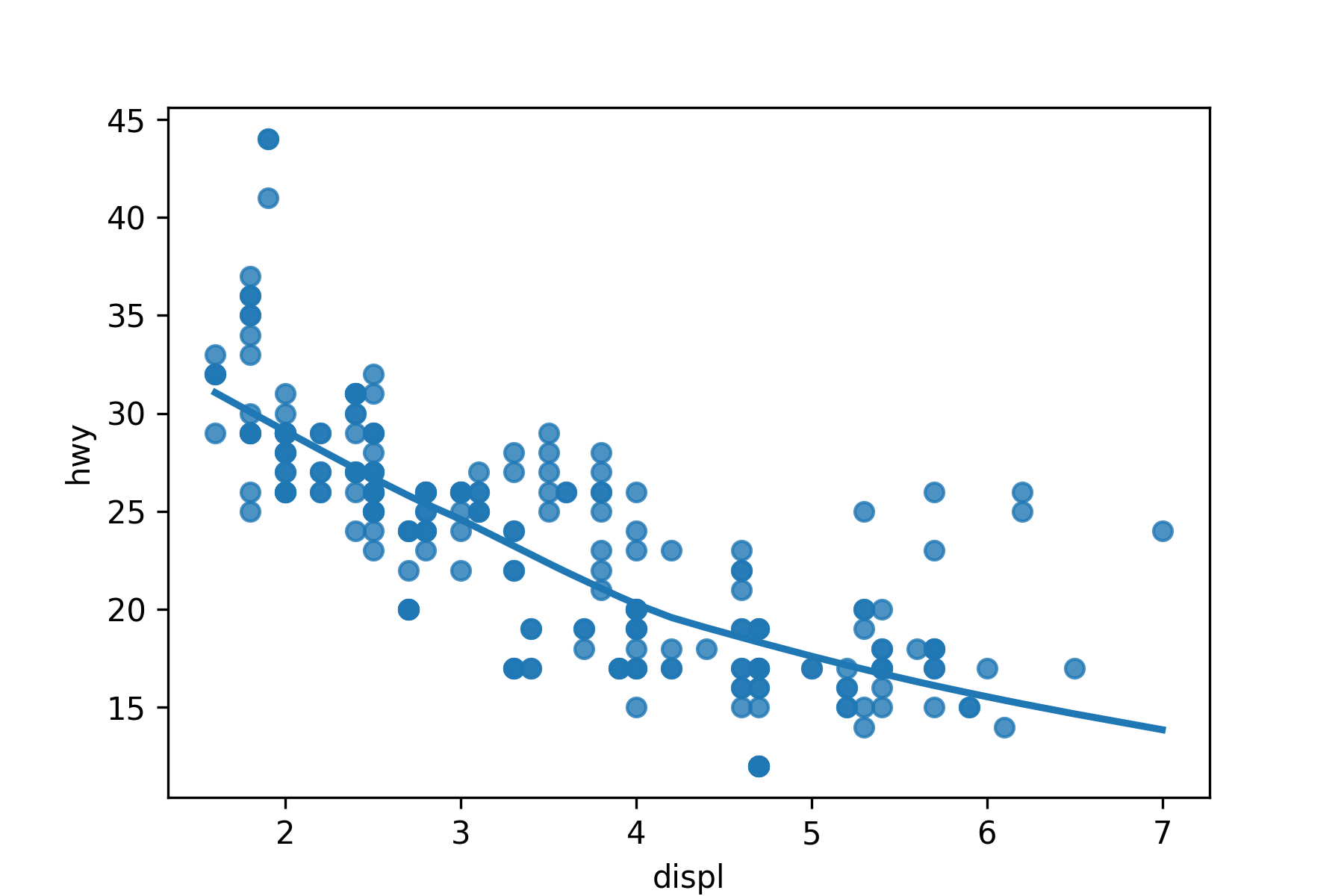
17.7.6 Lines/Smoothers
Use sns.regplot() to make a scatter plot with a regression line or a loess smoother.
- Regression line with 95% Confidence interval.
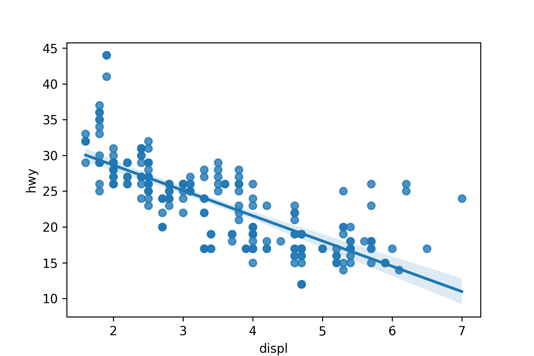
- Loess smoother with confidence interval removed.
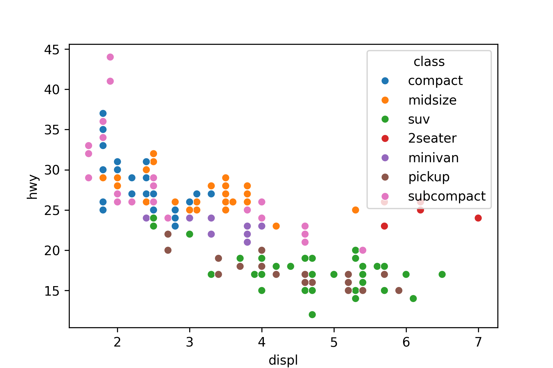
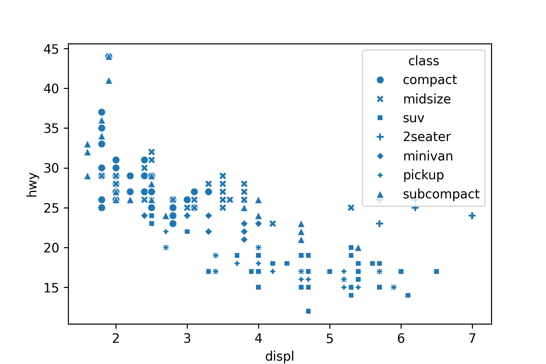
17.7.7 Annotating by a Third Variable
Use the hue or style arguments to annotate by a categorical variable:
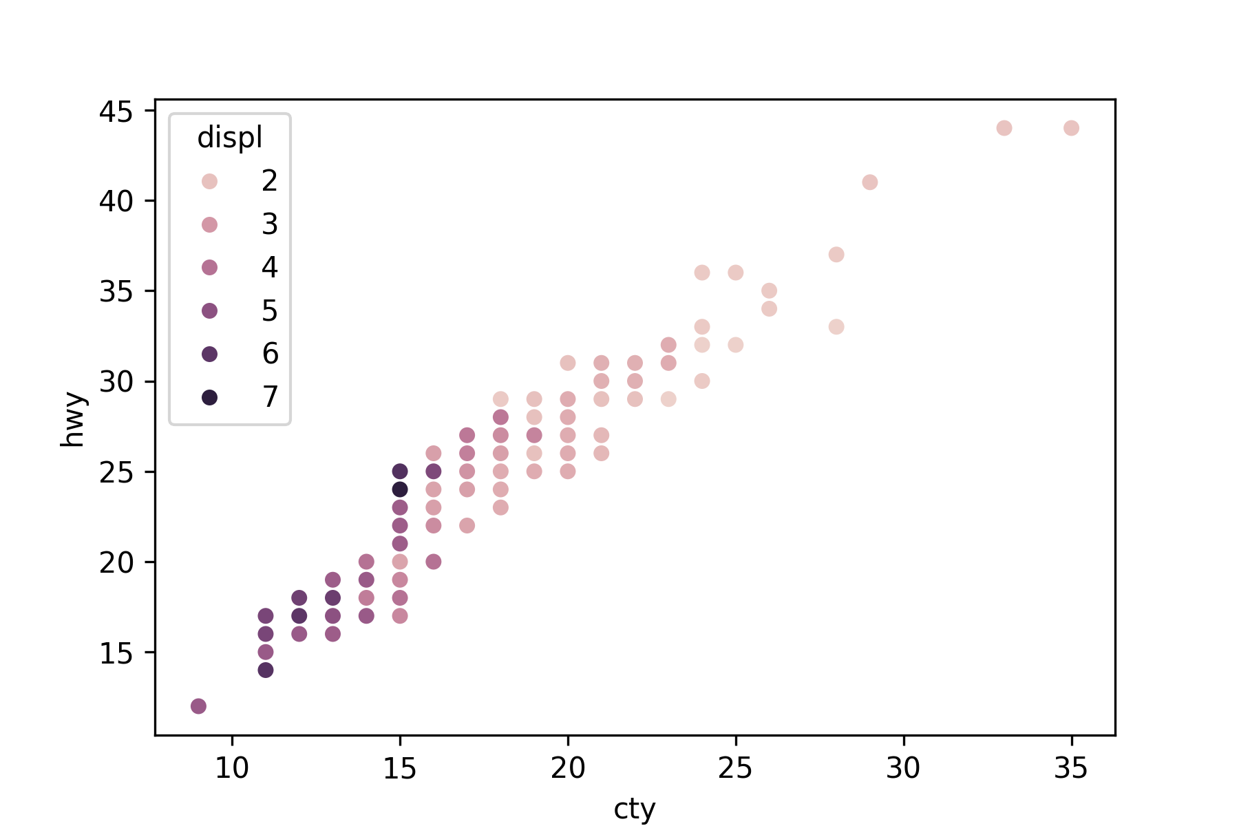
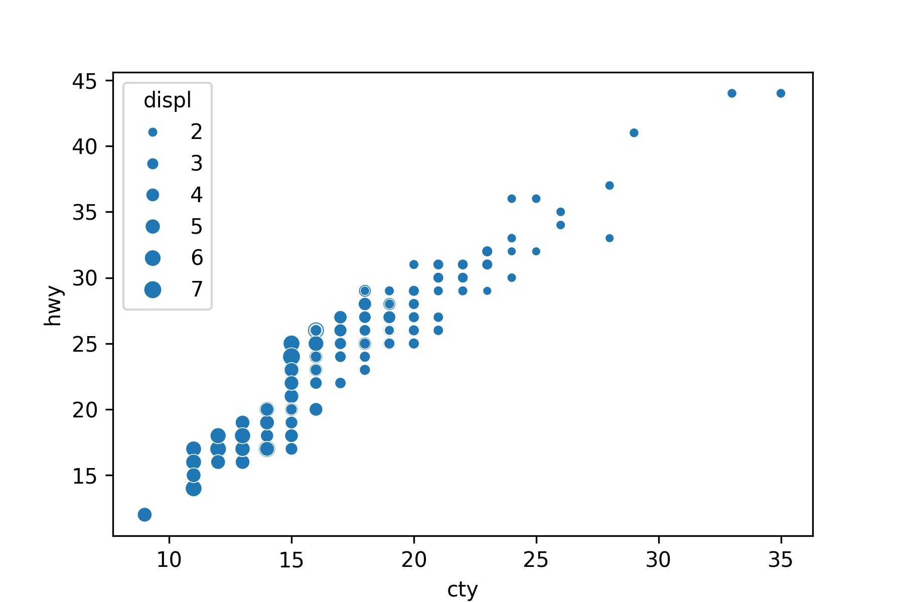
Use the hue or size arguments to annotate by a quantitative variable.
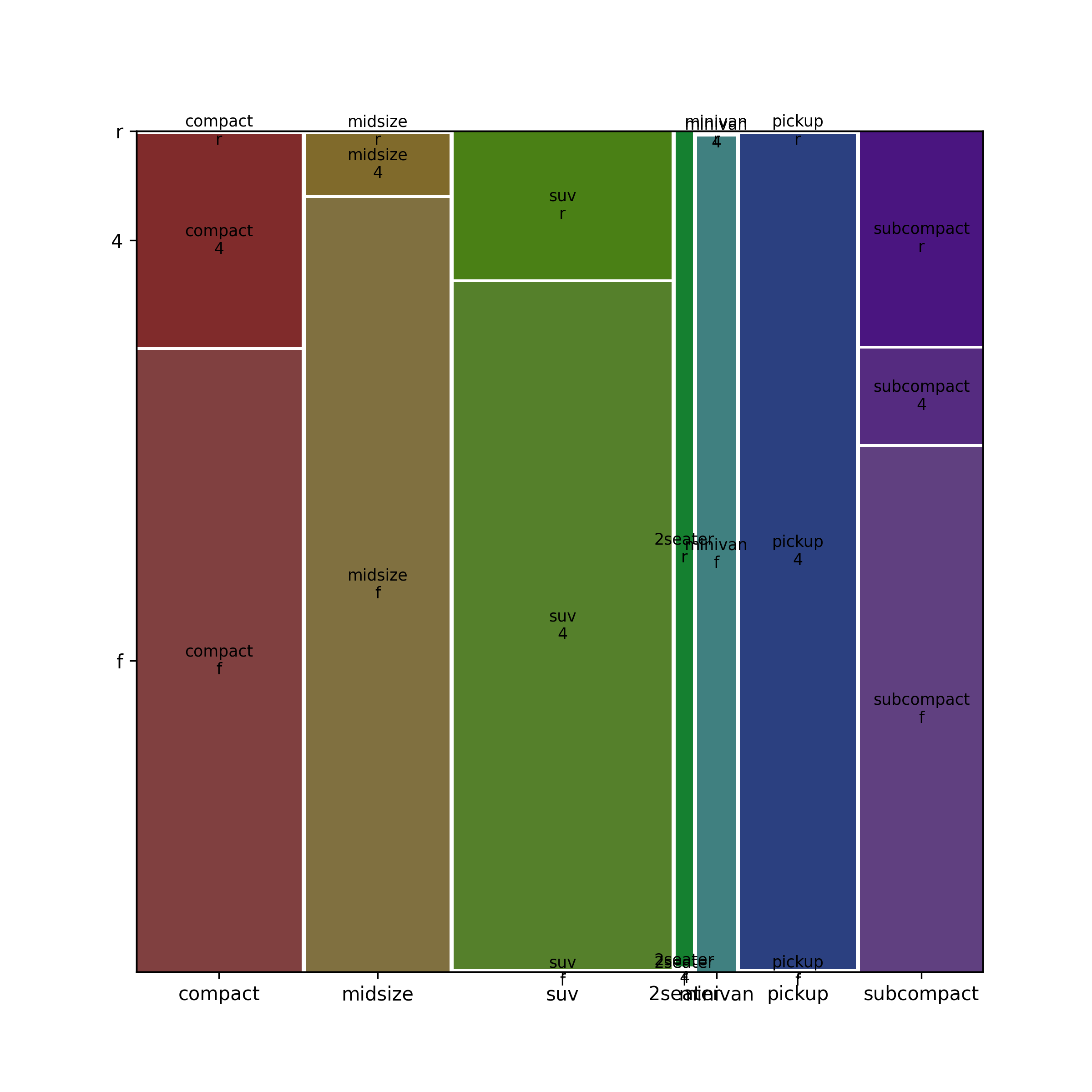
17.7.8 Two Categorical Variables: Mosaic Plot
When you want to plot two categorical variables, try a mosaic plot from the {statsmodels} package.
Import the plot object (and methods) from statsmodels.graphics.mosaicplot.
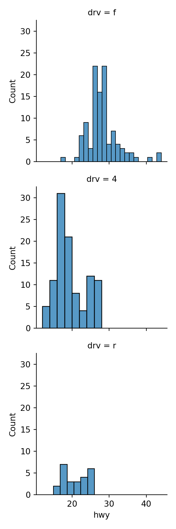
17.7.9 Facets
Use sns.FacetGrid() followed by the map() method to create faceted plots.
- The
FacetGridmethod creates the faceted plot structure and themap()method says how to assign the plot types and variables to the facets.
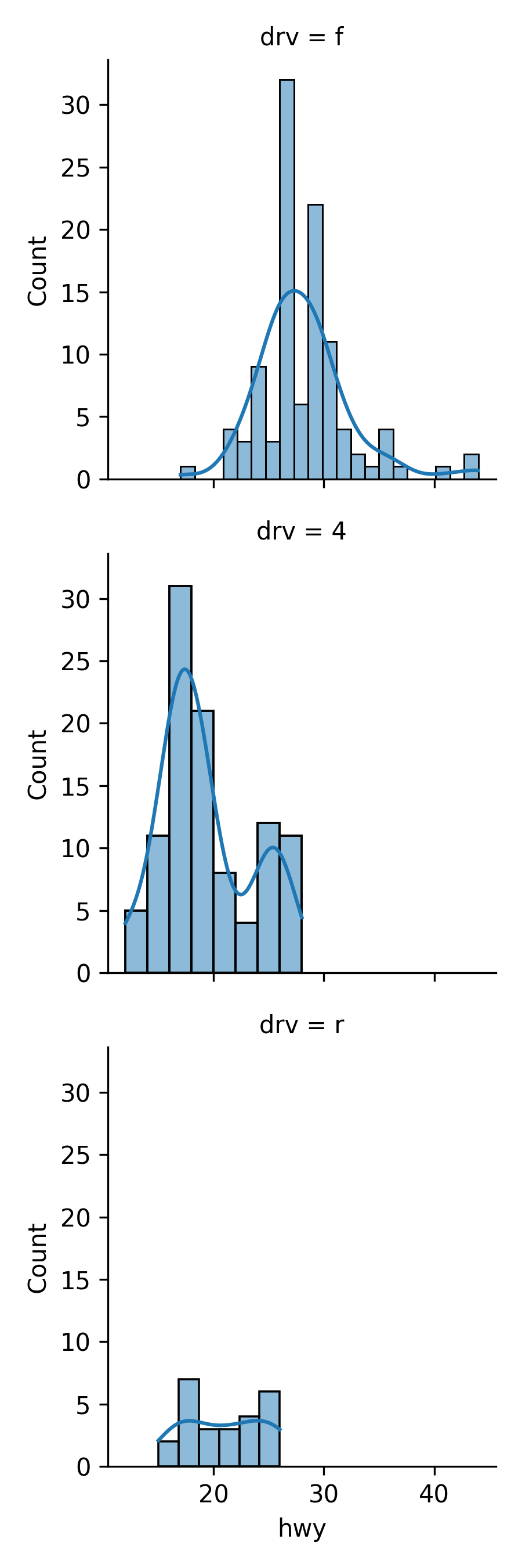
A density plot version.

17.7.10 Labels
Use plt.close() to close the figure window and start fresh.
You can add labels by assigning a plot to an object and then using set_*() methods to add labels.
17.7.11 Saving Figures
- First, assign a figure to an object.
- Extract the figure. Assign this to an object.
- Save the figure.
You can do all of these steps using piping.
- Note the use of
\to break the line instead of enclosing in().
17.8 Examples of R and Python
17.8.1 Running the Python Linear Model in R
The {scikit-learn} library was required in Listing 17.1.
Create a python script with the following code and save in a py directory.
from sklearn import linear_model as py_lmlinreg_python = py_lm.LinearRegression()Source the script in R with source_python() and a relative path.
Glimpse mtcars in R.
Rows: 32
Columns: 11
$ mpg  <dbl> 21.0, 21.0, 22.8, 21.4, 18.7, 18.1, 14.3, 24.4, 22.8, 19.2, 17.8,…
$ cyl  <dbl> 6, 6, 4, 6, 8, 6, 8, 4, 4, 6, 6, 8, 8, 8, 8, 8, 8, 4, 4, 4, 4, 8,…
$ disp <dbl> 160.0, 160.0, 108.0, 258.0, 360.0, 225.0, 360.0, 146.7, 140.8, 16…
$ hp   <dbl> 110, 110, 93, 110, 175, 105, 245, 62, 95, 123, 123, 180, 180, 180…
$ drat <dbl> 3.90, 3.90, 3.85, 3.08, 3.15, 2.76, 3.21, 3.69, 3.92, 3.92, 3.92,…
$ wt   <dbl> 2.620, 2.875, 2.320, 3.215, 3.440, 3.460, 3.570, 3.190, 3.150, 3.…
$ qsec <dbl> 16.46, 17.02, 18.61, 19.44, 17.02, 20.22, 15.84, 20.00, 22.90, 18…
$ vs   <dbl> 0, 0, 1, 1, 0, 1, 0, 1, 1, 1, 1, 0, 0, 0, 0, 0, 0, 1, 1, 1, 1, 0,…
$ am   <dbl> 1, 1, 1, 0, 0, 0, 0, 0, 0, 0, 0, 0, 0, 0, 0, 0, 0, 1, 1, 1, 0, 0,…
$ gear <dbl> 4, 4, 4, 3, 3, 3, 3, 4, 4, 4, 4, 3, 3, 3, 3, 3, 3, 4, 4, 4, 3, 3,…
$ carb <dbl> 4, 4, 1, 1, 2, 1, 4, 2, 2, 4, 4, 3, 3, 3, 4, 4, 4, 1, 2, 1, 1, 2,…
Check out the python linear regression function using View().
- Note: The function of a python package is accessed using
$symbol after the object into which the Python library is loaded. - This is very similar to how a column of a data frame is accessed using the
$operator.
Run the model in R using the python method fit for (mpg ~ everything_else).
- Separate the response
yand the explanatory variablex. - Note,
linreg_python$fitusesXfor the explanatory variables.
Look at the output.
Compare to R lm().
Check the R-squared in R.
17.8.1.1 Python Seaborn Plots in R using {reticulate}
Based on Python Seaborn Plots in R using reticulate.
The {ggplot2} package and the python package {seaborn} have different plots.
Use an R code chunk to import the requisite packages: {pandas}, {seaborn} and the {matplotlib} method called pyplot.
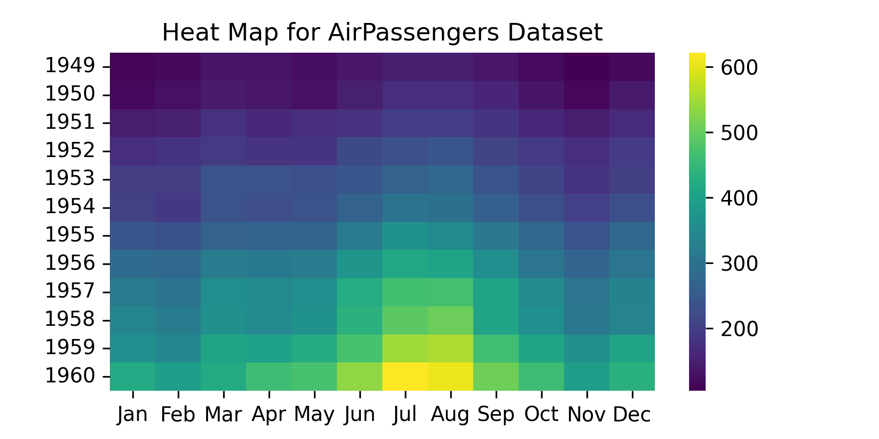
Let’s use R’s built-in AirPassengers dataset which is a time series object.
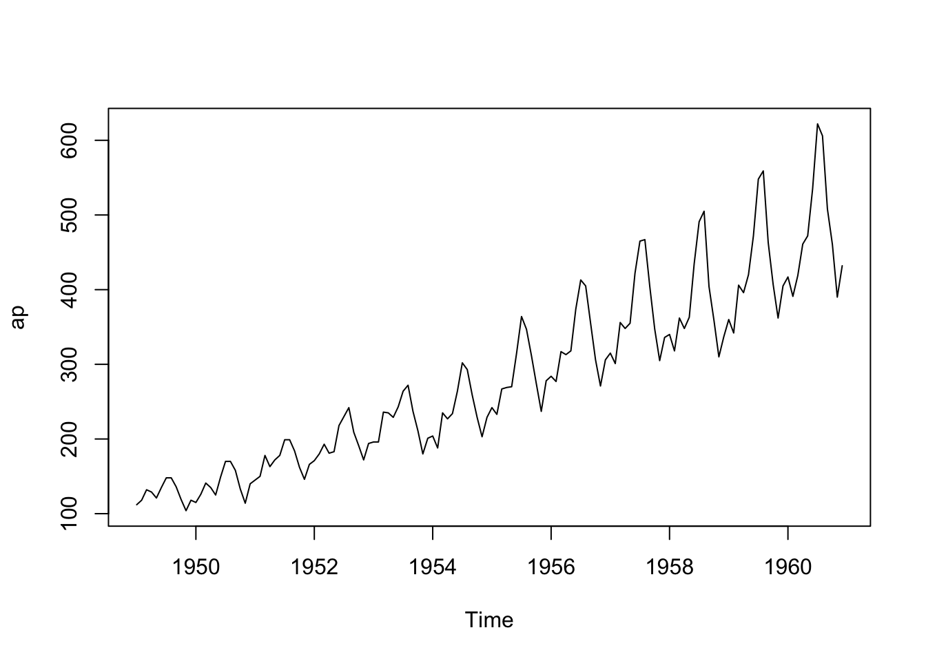
Convert the Time-Series object into an R data frame.
- See help for
ts(),time()andcycleas well as Transforming-a-time-series-into-a-data-frame-and-back.
17.8.1.1.1 Build a heatmap using {seaborn}.
- Use
r_to_py()to convert the R tibble into a python object.
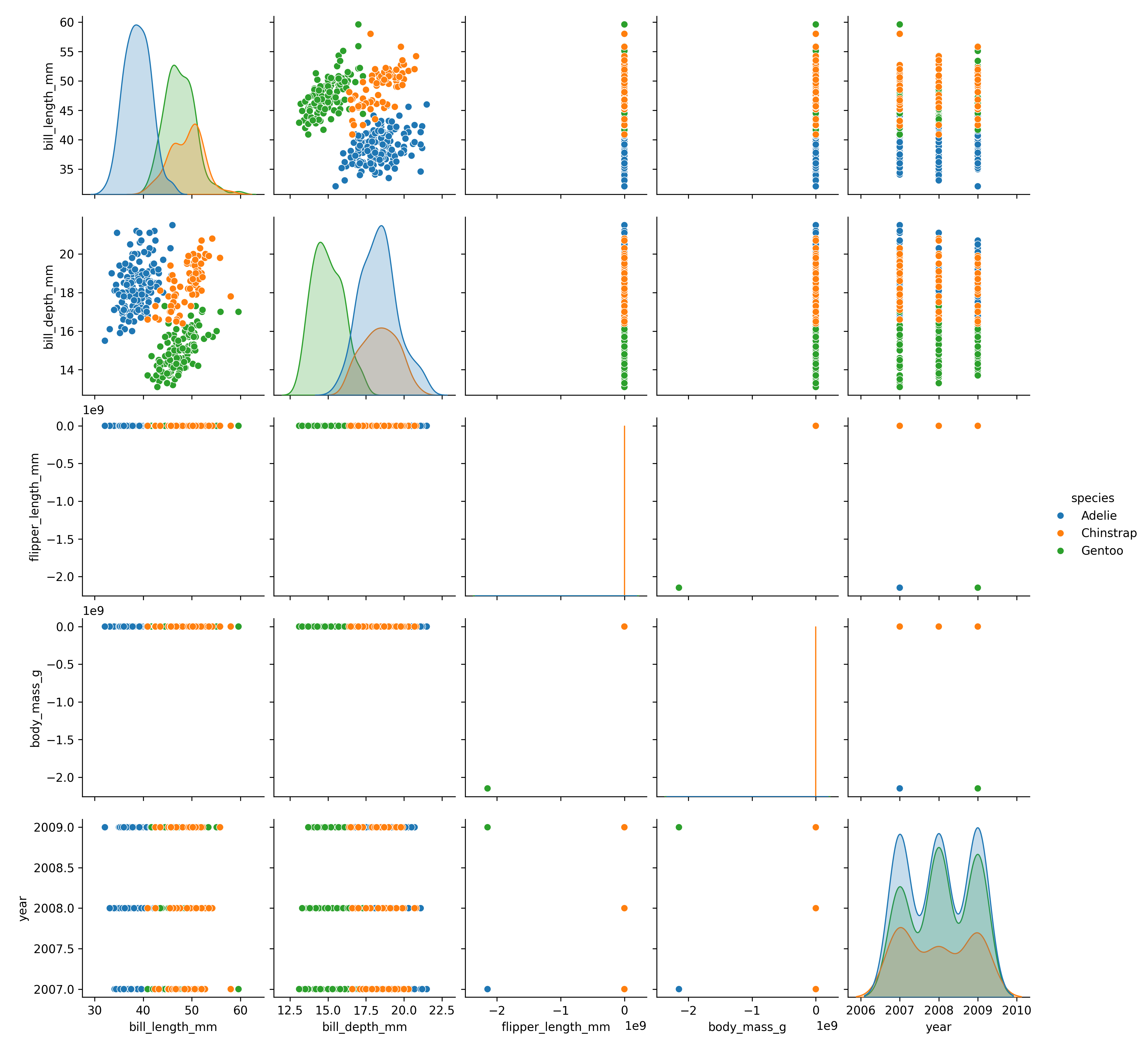
17.8.1.1.2 Build a seaborn pairplot using pairplot().
Attaching package: 'palmerpenguins'The following objects are masked from 'package:datasets':
penguins, penguins_rawDisplay the plot.
The seaborn plots you just saw were actually the result of a workaround suggested by the reticulate team (Tomasz Kalinowski) in response to a help request I submitted in June 2023 about why the plots were not rendering properly.
Thanks for filing. This is a current limitation of the interface. Within the reticulate knitr engine, we install hooks to customize plt.show() so that the figure appears in the rendered document. When evaluating plt$show() outside the reticulate knitr engine (that is, not in a python chunk), the hooks don’t get an opportunity to run so you get the default matplotlib behavior (showing the plot in a pop-up window).
Until this is fixed, you can work around this limitation by calling plt.show() in an (invisible) python chunk.
Create the plot in an R chunk. In a new R chunk set echo: true, eval: false with plt$show().
Follow that with a python chunk with echo: false, eval: true with import matplotlib.pyplot as plt and plt.show().
Using Python in R provides you flexibility in how you execute your analysis when you want capabilities not readily available in R.
17.9 Python Example from Quarto Documentation
This example is rendered using jupyter and not knitr but it is included in the overall set of notes files as just another file to be rendered.
R does not need to be installed for it to work.
17.9.1 Sample YAML
title: "matplotlib demo"
format: html
code-fold: true
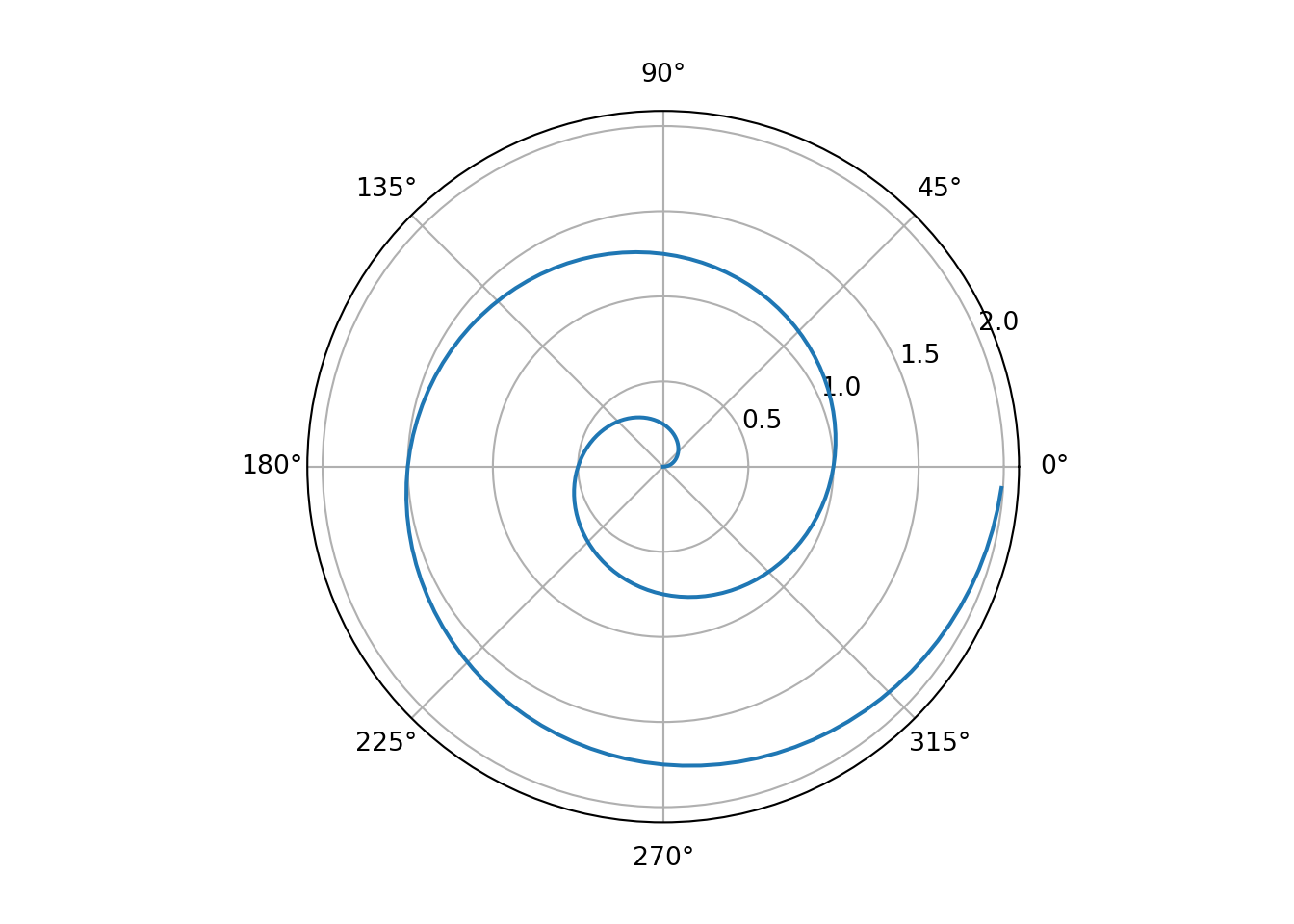
jupyter: python3For a demonstration of a line plot on a polar axis, see Figure 17.7.
```{python}
#| label: fig-polar
#| fig-cap: "A line plot on a polar axis"
#| message: false
import numpy as np
import matplotlib.pyplot as plt
import warnings # stop a future warning bug un seaborn from generating future warning messages
# see https://github.com/mwaskom/seaborn/issues/3486
warnings.simplefilter(action="ignore", category=FutureWarning)
r = np.arange(0, 2, 0.01)
theta = 2 * np.pi * r
fig, ax = plt.subplots(
subplot_kw = {'projection': 'polar'}
)
ax.plot(theta, r)
ax.set_rticks([0.5, 1, 1.5, 2])
ax.grid(True)
plt.show()
```