4 Lists and Iteration using R and {purrr}

Published

August 30, 2024

Keywords

vectors, lists, for-loops, purrr

4.1 Introduction

4.1.1 Learning Outcomes

Manipulate Vectors and Lists using Base R syntax.
Apply techniques of iteration using
- For-Loops in Base R
- map*() functions in the tidyverse {purrr} package

4.1.2 References:

R for Data Science 2nd Edition Wickham, Cetinkaya-Rundel, and Grolemund (2023)
Chapters 3 and 4 in Advanced R Wickham (2023)
Purrr Overview Wickham and Henry (2023)

4.1.2.1 Other References

Purrr Cheat Sheet

4.2 Review of Vectors

We’ll use just a few tidyverse functions.

library(tidyverse)

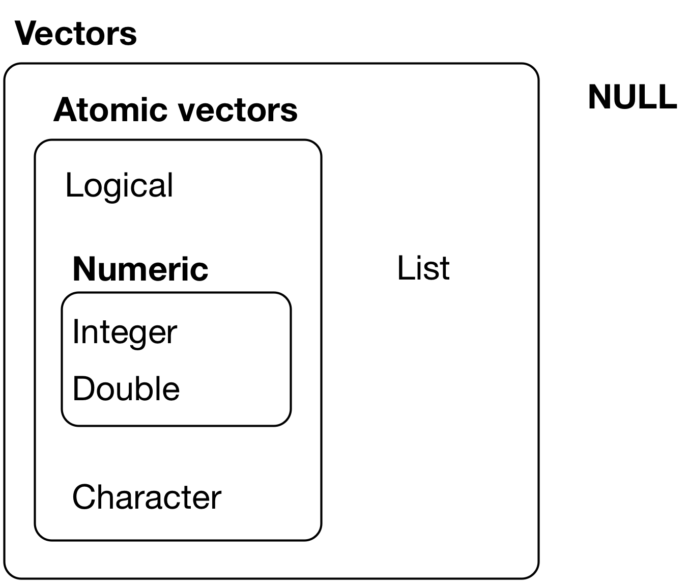
4.2.1 R has Two Kinds of Vectors: Atomic Vectors and Lists

Atomic vectors are sequences of elements of the same data type and class.

Lists are data structures where the elements do Not have to be the same class.

Sometimes called recursive vectors because lists can contain other lists!

Vectors have two main attributes: Length and data Type.

4.2.2 R has Six Data Types

The six data types are:

1.  logical,
2.  integer,
3.  double,
4.  character,
5.  complex, and
6.  raw(byte-level data).

factor, and date classes are special encodings of data types integer and double.
Integer and double vectors are collectively known as numeric vectors.

Missing Vectors return NULL, like missing or empty values in a vector can return NA.

R Vectors Wickham, Cetinkaya-Rundel, and Grolemund (2023)

4.2.3 Creating Vectors

Use c() to create a vector from the argument elements.

use length() to see the length of a vector.
Use typeof() to see the type of vector.
Use is_*() to check the type of vector (from package purrr).
- e.g., is_numeric(), is_logical, is.character, ….
- Base R has similar functions is.*().

4.2.3.1 Examples

Double:

    x <- c(1, 10, 2)
    length(x)

[1] 3

    typeof(x)

[1] "double"

    is_double(x) ### From purrr package

[1] TRUE

Integer: use L to tell R to treat (store) a number as an integer:

    x <- c(1L, 10L, 2L)
    typeof(x)

[1] "integer"

    is_integer(x) ### From purrr package

[1] TRUE

Character:

    x <- c("hello", "good", "sir")
    length(x)

[1] 3

    typeof(x)

[1] "character"

    is_character(x) ### From purrr package

[1] TRUE

Logical:

    x <- c(TRUE, FALSE, FALSE)
    typeof(x)

[1] "logical"

    is_logical(x) ### From purrr package

[1] TRUE

Factor: Factors are actually integers with extra attributes.

    x <- factor(c("A", "B", "B"))
    x

[1] A B B
Levels: A B

    typeof(x)

[1] "integer"

    is.factor(x)

[1] TRUE

    class(x)

[1] "factor"

    levels(x) ## to get the level labels

[1] "A" "B"

    as.numeric(x) ## to get the integers

[1] 1 2 2

Dates: Dates are actually doubles with extra attributes.

Dates are the number of days since January 1, 1970, with negative values for earlier dates.
The POSIXct class stores date/time values as the number of seconds since January 1, 1970.

    x <- lubridate::ymd(20150115, 20110630, 20130422)
    x

[1] "2015-01-15" "2011-06-30" "2013-04-22"

    length(x)

[1] 3

    typeof(x)

[1] "double"

    class(x)

[1] "Date"

    lubridate::is.Date(x)

[1] TRUE

    is_double(x) ### From purrr package

[1] TRUE

4.2.4 Working with Elements in a Vector

Each element of a vector can have a name.

    x <- c(horse = 7, man = 1, dog = 8)
    x

horse   man   dog 
    7     1     8

See and set/change element names with the names() function.

    names(x)

[1] "horse" "man"   "dog"

    names(x)[1] <- "cat"
    x

cat man dog 
  7   1   8

Subset with brackets [...].

Brackets are an extract or replace operator (see help for extract()).
The index object ... can be numeric, logical, character or empty.
Putting a logical vector inside the brackets returns (extracts) the elements from the outer vector where the corresponding value in the inner logical vector is TRUE.

    x <- c("I", "like", "dogs")
    x[2:3]

[1] "like" "dogs"

    lvec <- c(TRUE, FALSE, TRUE) 
    x[lvec]

[1] "I"    "dogs"

Replacement

    x[1] <- "You"
    x

[1] "You"  "like" "dogs"

    x[lvec] <- "We"
    x

[1] "We"   "like" "We"

Extract with negative values to drop elements.

    x[-3]

[1] "We"   "like"

Extract a named vector with the name(s) of the desired element(s) as a character vector.

    x <- c(horse = 7, man = 1, dog = 8)
    x[c("man", "horse")]

  man horse 
    1     7

Two brackets [[...]] only extracts a single element and drops the name.

The [[...]] operator performs the [...]operation twice.
Reduces an atomic vector to a named element and then extracts the element out of the named element.
Useful in working with lists (later on).

    x[3]

dog 
  8

    x[[3]]

[1] 8

4.2.4.1 Exercise

Create the following vector:

    x <- c(Yoshi = 10L,
           Mario = 31L,
           Luigi = 72L,
           Peach = 11L,
           Toad  = 38L)

Extract Yoshi and Peach from the above vector using:
1. Integer subsetting.
2. Negative integer subsetting.
3. Logical subsetting.
4. Name subsetting.

Show code

x[c(1, 4)]
x[c(-2, -3, -5)]
x[c(TRUE, FALSE, FALSE, TRUE, FALSE)]
x[c("Yoshi", "Peach")]

In the vector above, replace Yoshi’s number with 19L.

Show code

x["Yoshi"] <- 19L
x

4.2.5 Recycling

You are used to doing vectorized operations.

x <- c(1, 4, 1, 5)
x + 10

[1] 11 14 11 15

When operating on a vector with a scalar or two vectors of different lengths, R does what is called “recycling”.

Internally, R is reusing or “recycling” elements of the scalar or shorter vector to complete the operations. So the above example is treated the same as:

x + c(10, 10, 10, 10)

[1] 11 14 11 15

You can choose to recycle non-scalars, i.e., vectors of different lengths, but it’s almost never a good idea as R may not behave how you think it will.

It makes your code less robust to changes in the data structure over time, e.g., if someone added additional observations to the data:

x + c(10, 20)

[1] 11 24 11 25

x + c(10, 20, 10, 20, 30)

[1] 11 24 11 25 31

x + c(10, 20, 10, 20) ## no recycling required

[1] 11 24 11 25

4.3 Lists

4.3.1 Creating Lists

Lists are vectors whose elements can be of different types.

A tibble or data frame is a special kind of list (organized by columns with the same element types in them)

Use list() to make a list.

Each element in a list can have many elements (including other lists) in it.
The length of the list is just how many elements are present at the top level of the list.

my_first_list <- list(x = "a", y = 1, z = c(TRUE, FALSE, TRUE), list("a", 1))
my_first_list

$x
[1] "a"

$y
[1] 1

$z
[1]  TRUE FALSE  TRUE

[[4]]
[[4]][[1]]
[1] "a"

[[4]][[2]]
[1] 1

length(my_first_list)

[1] 4

The above list, of length 4, has three named elements: a character, a numeric, and a logical vector, and then it has an un-named list as the fourth element.

The internal unnamed list has two elements ("a", 1)and is also unnamed.

Use str() (for structure) to see the internal properties of a list.

str(my_first_list)

List of 4
 $ x: chr "a"
 $ y: num 1
 $ z: logi [1:3] TRUE FALSE TRUE
 $  :List of 2
  ..$ : chr "a"
  ..$ : num 1

If you have a deeply nested list, str() can produce a lot of output!

4.3.2 Working with Lists

Single brackets [...] extract a sublist. You use the same extracting strategies as for vectors.

my_first_list[1:2]

$x
[1] "a"

$y
[1] 1

str(my_first_list[1:2])

List of 2
 $ x: chr "a"
 $ y: num 1

my_first_list["y"]

$y
[1] 1

Double brackets [[...]] extract a single list element (which could also be a list).

Each set of brackets subsets one layer.

my_first_list[[1]]

[1] "a"

my_first_list[["z"]]

[1]  TRUE FALSE  TRUE

str(my_first_list[["z"]])

 logi [1:3] TRUE FALSE TRUE

Consider whether you want single [] or double [[]] when subsetting elements from a list.

Consider the list below.

Subsetting elements with a single set of brackets always returns a list with one element.
To remove the list layer, i.e., subset an element as its own structure, you must use two sets of brackets to remove the top layer of the list.

my_list <- list("a", mtcars[1:2, 1:2], list("c", "d"), mtcars[3:4, 3:4])

my_list[1]

[[1]]
[1] "a"

my_list[[1]]

[1] "a"

my_list[2] |> str()

List of 1
 $ :'data.frame':   2 obs. of  2 variables:
  ..$ mpg: num [1:2] 21 21
  ..$ cyl: num [1:2] 6 6

my_list[[2]] |> str()

'data.frame':   2 obs. of  2 variables:
 $ mpg: num  21 21
 $ cyl: num  6 6

my_list[3] |> str()

List of 1
 $ :List of 2
  ..$ : chr "c"
  ..$ : chr "d"

my_list[[3]] |> str()

List of 2
 $ : chr "c"
 $ : chr "d"

You can subset multiple elements of different classes with single [] but not multiple elements.

my_list[c(2, 3)] |> str()

List of 2
 $ :'data.frame':   2 obs. of  2 variables:
  ..$ mpg: num [1:2] 21 21
  ..$ cyl: num [1:2] 6 6
 $ :List of 2
  ..$ : chr "c"
  ..$ : chr "d"

my_list[[c(2, 4)]] |> str()

Error in my_list[[c(2, 4)]]: subscript out of bounds

Use dollar signs $ to extract named list elements (like in data frames).

my_first_list$z

[1]  TRUE FALSE  TRUE

Remove elements of a list by replacing them with NULL.

str(my_first_list)

List of 4
 $ x: chr "a"
 $ y: num 1
 $ z: logi [1:3] TRUE FALSE TRUE
 $  :List of 2
  ..$ : chr "a"
  ..$ : num 1

my_first_list$x <- NULL
str(my_first_list)

List of 3
 $ y: num 1
 $ z: logi [1:3] TRUE FALSE TRUE
 $  :List of 2
  ..$ : chr "a"
  ..$ : num 1

4.3.2.1 Exercise

Create the following list:

wedding <- list(venue = "chick-fil-a",
                guest = tribble(~name,     ~meal, ~age,
                                    ##--------/------/-----
                                    "Yoshi",   "V",   29L,
                                    "Wario",   "C",   27L,
                                    "Bowser",  "V",   34L,
                                    "Luigi",   "C",   36L,
                                    "Toad",    "B",   34L), 
                    bride = "Peach",
                    groom = "Mario",
                    date  = parse_date("11/10/2020", "%d/%m/%Y"))

Wario can’t actually make it.

Remove his row from the data frame.

Show code

wedding$guest |>
  filter(name != "Wario") ->
  wedding$guest
wedding$guest

Add a new named vector to the list.

Call it meal with the elements V is "Vegetarian", C is "Chicken", and B is "Beef".

Show code

wedding$meal <- c(V = "Vegetarian", C = "Chicken", B = "Beef")
wedding$meal

Extract the venue and the date from wedding.

Use three different techniques to do this.

Show code

wedding[c(1, 5)]
wedding[c("venue", "date")]
wedding$venue
wedding$date

"chick-fil-a" should be capitalized.

Capitalize the first "c" and last "a".

Show code

wedding$venue |>
  str_replace(pattern = "^c", "C") |> 
  str_replace(pattern = "a$", "A") -> 
  wedding$venue
wedding$venue
## or
wedding$venue |> 
  str_replace("^c(.+)a", "C\\1A") -> 
  wedding$venue

4.4 For-Loops in Base R

4.4.1 Motivation

Iteration is the repetition of some amount of code.
If we didn’t know the sum() function, how would we add up the elements of a vector?

x <- c(8, 1, 3, 1, 3)

We could manually add the elements.

x[1] + x[2] + x[3] + x[4] + x[5]

[1] 16

But this is prone to error (especially if we try to copy and paste multiple lines). Also, what if x has 10,000 elements?
For loops to the rescue! Here is an example:

[1] 8 1 3 1 3

sumval <- 0
for (i in seq_along(x)) {
  sumval <- sumval + x[[i]]
}
sumval

[1] 16

4.4.2 For-Loop Structure

For-loops are a standard means in multiple computer languages for iterating (repeating) sections of code for a specified number of iterations (repetitions)
Each for-loop contains the following elements:
1. Condition: This sets the number of iterations. It sets the values by which the loops will be sequenced (often by 1) and defines the variable by which the loops will be counted, normally variables such as i, j, or k.
- In the example above, the function seq_along(x) is a special version of seq which creates a vector from 1 to the length of x, incremented by 1 (so 1, 2, 3, 4, 5), and the variable i will contain each successive value from the vector as the loop iterates.
1. Body: This is the expression or code between the curly braces {}. This is the code will be evaluated each iteration with the new value of i for that iteration. After the end of the expression, the for loop increments the value of the index by the value set in the condition and checks if the loop needs to be run again. If the new value meets the condition, it executes the expression with the new value of i. If not, the for loop is complete and it moves to the line of code after the closing } of the for loop.
2. Output: The variable that is produced by the iteration. This is sumval above.
- It’s best to allocate the memory for the output before starting the for-loop.
In the above sequence, R internally transforms the code to:

sumval <- 0
sumval <- sumval + x[[1]]
sumval <- sumval + x[[2]]
sumval <- sumval + x[[3]]
sumval <- sumval + x[[4]]
sumval <- sumval + x[[5]]
sumval

[1] 16

There are four variations on the basic theme of the for loop:

Modifying an existing object, instead of creating a new object.
Looping over names or values, instead of indices.
Handling outputs of unknown length.
Handling sequences of unknown length.

A best practice for filling a new vector with values is to create it before you run the loop.

Create the new vector beforehand using the vector() function by specifying the type (mode) of the elements and the number of elements you need.
- Allocating memory is slow so it is faster to do it once before the loop than to add more memory with each iteration of the loop.
- Look at help for vector() and seq_along().
You can also create by assigning a vector of NAs but you should ensure they are of the correct type to avoid conversion during the loop. See help for NA.

For example, let’s calculate a vector of the cumulative sums each element in x.

The for loop sets the condition and then checks if i ==1.
If so, it executes the next line. If not, it jumps to the else line.
At the end of the expression, it increments i by 1, so i = i +1 and goes back to the line with the for loop condition.
It checks if the new value of i still meets the condition. If so, it executes the expression again. If not, the for loop is done and it jumps to the line of code after the for loop ending }.

## Allocate the memory in a new variable
cumvec <- vector(mode = "double", length = length(x))
cumvec

[1] 0 0 0 0 0

## start the for-loop
for (i in seq_along(cumvec)) {
  if (i == 1) {
    cumvec[[i]] <- x[[i]]
  } else {
    cumvec[[i]] <- cumvec[[i - 1]] + x[[i]]
  }
}
cumvec

[1]  8  9 12 13 16

### Same result as cumsum(x)
cumsum(x)

[1]  8  9 12 13 16

The first two numbers of the Fibonacci Sequence are 0 and 1. Each succeeding number is the sum of the previous two numbers in the sequence. For example, the third element is 0 + 1 = 1, while the fourth element is 1 + 1 = 2, and the fifth element is 2 + 1 = 3 and so on.

Use a for loop to calculate the first 100 Fibonacci Numbers.
As a sanity check: The $\log_2$ of the 100^th Fibonacci Number is about 67.57.
Design your steps - there are two alternatives: Set the first two values inside the loop or set them outside the loop
1. Initialize an empty vector of the desired length to hold your numbers
2. If you initialize outside the loop, do it now.
3. Create your for loop to iterate as many times as you need.
4. Create the logic to compute the numbers.

Show code

fibvec <- vector(mode = "double", length = 100)
for (i in seq_along(fibvec)) {
  if (i > 2) {
    fibvec[[i]] <- fibvec[[i - 1]] + fibvec[[i - 2]]
  } else if (i == 1) {
    fibvec[[i]] <- 0
  } else if (i == 2) {
    fibvec[[i]] <- 1
  } else {
    stop(paste0("i = ", i))
  }
}

## Test the results
head(fibvec, n = 10)
log2(fibvec[100])

fibvec <- vector(mode = "double", length = 100)
## initialize outside the loop
fibvec[1:2] <- c(0, 1)
## run the loop skipping the first two numbers
for (i in seq(from = 3, to = length(fibvec))) {
  fibvec[[i]] <- fibvec[[i - 1]] + fibvec[[i - 2]]
}

## Test the results
head(fibvec, n = 10)
log2(fibvec[100])

4.4.3 Looping Over the Columns of a Data Frame.

For a data frame df, seq_along(df) is the same as 1:ncol(df) which is the same as 1:length(df) (since data frames are special cases of lists).

Let’s calculate the mean of each column of mtcars.

mean_vec <- vector(mode = "numeric", length = length(mtcars))
for (i in seq_along(mtcars)) {
  mean_vec[[i]] <- mean(mtcars[[i]], na.rm = TRUE)
}
mean_vec

 [1]  20.090625   6.187500 230.721875 146.687500   3.596563   3.217250
 [7]  17.848750   0.437500   0.406250   3.687500   2.812500

colMeans(mtcars)

       mpg        cyl       disp         hp       drat         wt       qsec 
 20.090625   6.187500 230.721875 146.687500   3.596563   3.217250  17.848750 
        vs         am       gear       carb 
  0.437500   0.406250   3.687500   2.812500

Why not just use colMeans()? Well, you could if you only wanted means.

However, if you wanted column standard deviations, there is no “colSDs” function.
Thus you needed some form of iteration for applying custom functions to multiple elements.

For-loops are one method for iteration.

sd_vec <- vector(mode = "numeric", length = length(mtcars))
for (i in seq_along(mtcars)) {
  sd_vec[[i]] <- sd(mtcars[[i]], na.rm = TRUE)
}
sd_vec

 [1]   6.0269481   1.7859216 123.9386938  68.5628685   0.5346787   0.9784574
 [7]   1.7869432   0.5040161   0.4989909   0.7378041   1.6152000

Good News! With {dplyr} 1.0 we can now use across() as another approach to iteration for many functions.

Let’s load the {tidyverse} which should have {dplyr} version 1.1.2 or greater.

library(tidyverse)

Look at help for across() and/or the Column-wise vignette to learn about across() and its counterpart rowwise().

Use across() inside a call to summarize() or mutate().

Note the fn argument of where() is the name of the function - do not include the paren operator which “calls” the function.

mtcars  |> 
  ##  group_by(cyl)  |> 
  summarize(across(where(is.numeric), sd),
    .groups = "drop"
  )

       mpg      cyl     disp       hp      drat        wt     qsec        vs
1 6.026948 1.785922 123.9387 68.56287 0.5346787 0.9784574 1.786943 0.5040161
         am      gear   carb
1 0.4989909 0.7378041 1.6152

So, you no longer need write a for-loop to do complex summaries of columns, but there are many times when iteration is the best approach to accomplish a desired transformation of the data.

4.4.3.1 Exercise

Use a for-loop to calculate the standard deviation of the four numeric traits in columns 3 to 6 of the penguins data frame from {palmerpenguins}.

Repeat using across() using where() to limit to numeric columns.
What is different about the results?

Show code

data(penguins, package = "palmerpenguins")
sdvec <- rep(NA_real_, length = 4)
for (i in seq_along(sdvec)) {
  sdvec[i] <- sd(penguins[[i + 2]], na.rm = TRUE)
}
sdvec

penguins  |> 
  summarize(across(where(is.numeric), .fns = ~ sd(.x, na.rm = TRUE)))

# for loop creates a vector and across creates a data frame.

4.4.4 The `while()` function as an alternative

Sometimes you don’t know how many times to repeat the code block as it may depend upon the results of the loop.

You might want to loop until you get three heads in a row in a simulation, or,
You might want to loop until the difference between two values is below or above some threshold.
You can’t do that sort of iteration with the for-loop. Instead, use a while-loop.

A while loop is simpler than for loop because it only has two components, a condition and a body.

```{r}
#| eval: false
while (condition) {
  ## body
}
```

A while-loop is also more general than a for-loop, because you can rewrite any for-loop as a while-loop, but you can’t rewrite every while-loop as a for-loop.

Example: Use a while-loop to find how many tosses of a coin it takes till one gets three heads in a row:

set.seed(1)
flip <- function() sample(c("T", "H"), 1)

flips <- 0
nheads <- 0

while (nheads < 3) {
  if (flip() == "H") {
    nheads <- nheads + 1
  } else {
    nheads <- 0 # start over
  } ## end else
  flips <- flips + 1
} ## end while loop
flips

[1] 18

4.5 Using the {purrr} Package for Iteration

4.5.1 Intro to the {purrr} Package

R is a functional programming language

You can pass functions to functions and use functions to create or change functions.
You can compose functions together to effect what happens in the environment.

Suppose for the mtcars data frame, we want to calculate the column-wise mean, the column-wise median, the column-wise standard deviation, the column-wise maximum, the column-wise minimum, and the column-wise median absolute deviation MAD.

The for-loop would look very similar for each function fun as shown in this non-executable example.

  ## Dummy Code with a generic "fun()" function

  funvec <- rep(NA_real_, length = length(mtcars))
  for (i in seq_along(funvec)) {
    funvec[i] <- fun(mtcars[[i]], na.rm = TRUE)
  }
  funvec

Ideally, we would like to just tell R what function to apply to each column of mtcars instead of writing all the code for a for-loop.

This is exactly what the {purrr} package allows us to do:

{purrr} provides a consistent syntax for identifying a set of data and then a function to be applied to that data.
{purrr} is a part of the {tidyverse} package so does not need to be loaded separately.

library(tidyverse)

4.5.2 The {purrr} `map` Functions

The {purrr} functions that start with map (known as the map*() functions) use the same four arguments

.x: a list or atomic vector with one or more elements. .x can be a vector, a data frame, or a list.
.f: a function you want to apply to each of the elements of the .x data structure.
...: a placeholder for additional arguments to be passed to the .f function, e.g., na.rm=TRUE.
.progress: A TRUE/FALSE logical for whether to show a progress bar during execution.

The .f functions can be:

a named function from Base R or an R package present in the global environment or accessible using package::function().
a named function you wrote that is accessible in the environment (has been sourced).
an unnamed or “anonymous function” you define inside the map function. These can include those defined with the new anonymous function shorthand backslash \().

Note

As of version 1.0 (Dec 2022), the the formula syntax with the ~ operator and . pronoun is no longer recommended.

The anonymous function shorthand syntax \(arg) expr with explicit arguments is now recommended.

The map*() functions do the work of running a for-loop for you.

They create the necessary data structures (and memory) of the desired type.
They break out the .x data structure into its top level elements.
- A .x vector becomes the individual elements of the vector .x[1], .x[2], ...
- A .x data frame becomes the individual columns of the data frame, df[,1], df[,2], ...
- A .x list becomes the individual elements of the list, which could be their own individual values, vectors, data frames or lists.
They iterate to pass each of the individual elements as an input argument to the .f function, e.g.,
- the i^th element returns the output of .f(.x[i], ...) as the i^th element of the designated output structure.
They return the output in the desired form and type.
- The output has the same number of elements as the original .x but may be of a different form, e.g., the .f() function may summarize columns of a data frame into a vector.

The different variants of the map_* function return different forms of output.
- map() always returns a list.
- map_lgl() returns a logical vector.
- map_int() returns an integer vector.
- map_dbl() returns a double vector.
- map_chr() returns a character vector.
- map_vec() returns an atomic vector for use when .f returns classes such as dates, factors, and date-times. You can use the ptype= (prototype) argument to specify the class.

The use of map_* allows you to write succinct code such as the following.

## .x is mtcars, a data frame so it breaks out into columns
## .f is the function below which is applied to each column of mtcars
map(.x = mtcars, .f = mean)
map_dbl(.x = mtcars, .f = mean)
map_dbl(mtcars, median)
map_dbl(mtcars, sd)
map_dbl(mtcars, mad)
map_dbl(mtcars, min)
map_dbl(mtcars, max)

By using the ... argument, you can pass on more arguments to map_*() so they can be passed to the .f function.

map_dbl(mtcars, mean, na.rm = TRUE)

       mpg        cyl       disp         hp       drat         wt       qsec 
 20.090625   6.187500 230.721875 146.687500   3.596563   3.217250  17.848750 
        vs         am       gear       carb 
  0.437500   0.406250   3.687500   2.812500

## equivalent to mean(mtcars[,i], na.rm = TRUE) for each of i columns

As an example, you can use map to get the output of summary() on each column.

map(.x = mtcars, .f = summary)

Exercise
Code Solution

Write code using one of the map functions to:
1. Create a character vector with the type of each column in nycflights13::flights.
2. Create an integer vector with the number of unique values in each column of Toothgrowth from the base R {datasets} package.
Repeat 1 and 2 using dplyr::across() without using map*().

Show code

data("flights", package = "nycflights13")
data("ToothGrowth", package = "datasets")

map_chr(flights, typeof)
map_int(ToothGrowth, function(x) length(unique(x)))

summarize(flights, across(.cols = everything(), typeof))

ToothGrowth |>
  summarize(across(.cols = everything(), ~ length(unique(.))))

4.5.3 Why Use {purrr}?

The chief benefit of using map*() functions instead of for-loops is clarity, not speed; they can make your code easier to write, read, and maintain as the intent is clearer.

The focus is on the operation being performed, e.g., mean(), not the coding the bookkeeping required to create an output vector, set conditions, loop over every element, and capture the iterated output.

Base R has the apply family of functions that are similar. Using {purrr} functions offers some advantages.

{purrr} functions have consistent names and arguments and work well with other tidyverse functions.
The first argument is always the data, so {purrr} works with the pipe.
{purrr} functions use . as an argument prefix to avoid inadvertently mixing {purrr} function arguments with those of the .f function.
{purrr} functions provide for all combinations of input and output variants and have specific map2_* functions for the common two argument case.
{purrr} functions are written in C so can be faster than other options.
See purrr base R for more details.

When performing operations on the columns of a data frame, the dplyr::across()function is an option besides using {purrr}.

4.5.4 {purrr} Functions for Working with Lists

The inherent flexibility of the list data structure can make working with them both necessary and challenging.

Deeply nested lists are commonly used to capture the complexity of a data set while minimizing redundancy and storage.
However, deeply nested lists can be hard to operate on with other functions.

Flattening and simplification are operations on lists to expose the data of interest in a convenient form.

Version 1.0 of {purrr} superseded the dfc and dfr functions for creating data frames with three new sets of functions for working with lists:

list_flatten() removes a single level of hierarchy from a list; the output is always a list.
- This means it collapses lower level lists into the parent element above them.
list_simplify() reduces a list to a homogeneous vector; the output is always the same length as the input.
- This means all the list elements must have length 1.
list_c(), list_cbind(), and list_rbind() concatenate the elements of a list to produce a vector or data frame.
- list_c concatenates all the elements into an atomic vector so they must be of the same class.
- list_cbind() and list_rbind() only work with lists where every element is a data frame.
- list_cbind() takes the elements and concatenates them as columns so they must each have of the same length.
- list_rbind() takes the elements and concatenates them as rows.
  - If a row is missing a column, it will fill with NA.
  - You have to be careful with how names are assigned (see help).

Example of list_flatten() showing you can use it to keep removing lower level lists until the list is as flat as possible.

x <- list(1, list(2, list(3, 4), 5))
x |> str()

List of 2
 $ : num 1
 $ :List of 3
  ..$ : num 2
  ..$ :List of 2
  .. ..$ : num 3
  .. ..$ : num 4
  ..$ : num 5

x |>
  list_flatten() |>
  str()

List of 4
 $ : num 1
 $ : num 2
 $ :List of 2
  ..$ : num 3
  ..$ : num 4
 $ : num 5

x |>
  list_flatten() |>
  list_flatten() |>
  str()

List of 5
 $ : num 1
 $ : num 2
 $ : num 3
 $ : num 4
 $ : num 5

x |>
  list_flatten() |>
  list_flatten() |>
  list_flatten() |>
  str()

List of 5
 $ : num 1
 $ : num 2
 $ : num 3
 $ : num 4
 $ : num 5

x |>
  list_flatten() |>
  list_flatten() |>
  list_simplify() |> 
  str()

 num [1:5] 1 2 3 4 5

Examples of the concatenation functions.

Let’s create a list of three data frames using split().
split(.$cyl) is a base R function to turn a data frame into a list of data frames where each data frame has a different value for all units based on the f = argument.
The “.” in split references the current data frame (since split() is not tidyverse).
Note the data frames have the same length but different numbers of observations.

mtcars_s <- split(mtcars, f = mtcars$cyl)
str(mtcars_s)

List of 3
 $ 4:'data.frame':  11 obs. of  11 variables:
  ..$ mpg : num [1:11] 22.8 24.4 22.8 32.4 30.4 33.9 21.5 27.3 26 30.4 ...
  ..$ cyl : num [1:11] 4 4 4 4 4 4 4 4 4 4 ...
  ..$ disp: num [1:11] 108 146.7 140.8 78.7 75.7 ...
  ..$ hp  : num [1:11] 93 62 95 66 52 65 97 66 91 113 ...
  ..$ drat: num [1:11] 3.85 3.69 3.92 4.08 4.93 4.22 3.7 4.08 4.43 3.77 ...
  ..$ wt  : num [1:11] 2.32 3.19 3.15 2.2 1.61 ...
  ..$ qsec: num [1:11] 18.6 20 22.9 19.5 18.5 ...
  ..$ vs  : num [1:11] 1 1 1 1 1 1 1 1 0 1 ...
  ..$ am  : num [1:11] 1 0 0 1 1 1 0 1 1 1 ...
  ..$ gear: num [1:11] 4 4 4 4 4 4 3 4 5 5 ...
  ..$ carb: num [1:11] 1 2 2 1 2 1 1 1 2 2 ...
 $ 6:'data.frame':  7 obs. of  11 variables:
  ..$ mpg : num [1:7] 21 21 21.4 18.1 19.2 17.8 19.7
  ..$ cyl : num [1:7] 6 6 6 6 6 6 6
  ..$ disp: num [1:7] 160 160 258 225 168 ...
  ..$ hp  : num [1:7] 110 110 110 105 123 123 175
  ..$ drat: num [1:7] 3.9 3.9 3.08 2.76 3.92 3.92 3.62
  ..$ wt  : num [1:7] 2.62 2.88 3.21 3.46 3.44 ...
  ..$ qsec: num [1:7] 16.5 17 19.4 20.2 18.3 ...
  ..$ vs  : num [1:7] 0 0 1 1 1 1 0
  ..$ am  : num [1:7] 1 1 0 0 0 0 1
  ..$ gear: num [1:7] 4 4 3 3 4 4 5
  ..$ carb: num [1:7] 4 4 1 1 4 4 6
 $ 8:'data.frame':  14 obs. of  11 variables:
  ..$ mpg : num [1:14] 18.7 14.3 16.4 17.3 15.2 10.4 10.4 14.7 15.5 15.2 ...
  ..$ cyl : num [1:14] 8 8 8 8 8 8 8 8 8 8 ...
  ..$ disp: num [1:14] 360 360 276 276 276 ...
  ..$ hp  : num [1:14] 175 245 180 180 180 205 215 230 150 150 ...
  ..$ drat: num [1:14] 3.15 3.21 3.07 3.07 3.07 2.93 3 3.23 2.76 3.15 ...
  ..$ wt  : num [1:14] 3.44 3.57 4.07 3.73 3.78 ...
  ..$ qsec: num [1:14] 17 15.8 17.4 17.6 18 ...
  ..$ vs  : num [1:14] 0 0 0 0 0 0 0 0 0 0 ...
  ..$ am  : num [1:14] 0 0 0 0 0 0 0 0 0 0 ...
  ..$ gear: num [1:14] 3 3 3 3 3 3 3 3 3 3 ...
  ..$ carb: num [1:14] 2 4 3 3 3 4 4 4 2 2 ...

list_c() concatenates the three data frames from the list back into one data frame.

list_c(mtcars_s) |> head()

                mpg cyl  disp hp drat    wt  qsec vs am gear carb
Datsun 710     22.8   4 108.0 93 3.85 2.320 18.61  1  1    4    1
Merc 240D      24.4   4 146.7 62 3.69 3.190 20.00  1  0    4    2
Merc 230       22.8   4 140.8 95 3.92 3.150 22.90  1  0    4    2
Fiat 128       32.4   4  78.7 66 4.08 2.200 19.47  1  1    4    1
Honda Civic    30.4   4  75.7 52 4.93 1.615 18.52  1  1    4    2
Toyota Corolla 33.9   4  71.1 65 4.22 1.835 19.90  1  1    4    1

list_rbind() concatenates the three data frames from the list back into one data frame as well since they have the same column structure.

list_rbind(mtcars_s) |> head()

                mpg cyl  disp hp drat    wt  qsec vs am gear carb
Datsun 710     22.8   4 108.0 93 3.85 2.320 18.61  1  1    4    1
Merc 240D      24.4   4 146.7 62 3.69 3.190 20.00  1  0    4    2
Merc 230       22.8   4 140.8 95 3.92 3.150 22.90  1  0    4    2
Fiat 128       32.4   4  78.7 66 4.08 2.200 19.47  1  1    4    1
Honda Civic    30.4   4  75.7 52 4.93 1.615 18.52  1  1    4    2
Toyota Corolla 33.9   4  71.1 65 4.22 1.835 19.90  1  1    4    1

list_cbind() generates an error as the three data frames from the list have different numbers of rows so can’t fit in the same column structure.

list_cbind(mtcars_s)

Error in `list_cbind()`:
! Can't recycle `4` (size 11) to match `6` (size 7).

This example from the list_cbind()help shows that list_cbind() returns a data frame with packed columns where the packed data frames retain the names of the original list elements and their columns retain the names from the original data frame.

You can still access these columns directly though the names and subsetting.

x2 <- list(
  a = data.frame(x = 1:2),
  b = data.frame(y = "a")
)
list_cbind(x2) -> x2_df
x2_df |> str()

'data.frame':   2 obs. of  2 variables:
 $ a:'data.frame':  2 obs. of  1 variable:
  ..$ x: int  1 2
 $ b:'data.frame':  2 obs. of  1 variable:
  ..$ y: chr  "a" "a"

x2_df |> names()

[1] "a" "b"

x2_df$a |> str()

'data.frame':   2 obs. of  1 variable:
 $ x: int  1 2

x2_df$a |> names()

[1] "x"

x2_df[1]

  x
1 1
2 2

x2_df[[1]]

  x
1 1
2 2

You can also unpack the data frame columns with tidyr::unpack().

Again you have to be careful with how to manage the names.

unpack(x2_df, cols = everything()) -> x2_un
x2_un |> str() # note the data frame names a and b are gone.

tibble [2 × 2] (S3: tbl_df/tbl/data.frame)
 $ x: int [1:2] 1 2
 $ y: chr [1:2] "a" "a"

x2_un |> names()

[1] "x" "y"

x2_un$x

[1] 1 2

This example shows list_cbind() with a larger data set, dplyr::starwars.

We drop the list columns (12-14) as they cannot be converted to data frames.

glimpse(dplyr::starwars)

Rows: 87
Columns: 14
$ name       <chr> "Luke Skywalker", "C-3PO", "R2-D2", "Darth Vader", "Leia Or…
$ height     <int> 172, 167, 96, 202, 150, 178, 165, 97, 183, 182, 188, 180, 2…
$ mass       <dbl> 77.0, 75.0, 32.0, 136.0, 49.0, 120.0, 75.0, 32.0, 84.0, 77.…
$ hair_color <chr> "blond", NA, NA, "none", "brown", "brown, grey", "brown", N…
$ skin_color <chr> "fair", "gold", "white, blue", "white", "light", "light", "…
$ eye_color  <chr> "blue", "yellow", "red", "yellow", "brown", "blue", "blue",…
$ birth_year <dbl> 19.0, 112.0, 33.0, 41.9, 19.0, 52.0, 47.0, NA, 24.0, 57.0, …
$ sex        <chr> "male", "none", "none", "male", "female", "male", "female",…
$ gender     <chr> "masculine", "masculine", "masculine", "masculine", "femini…
$ homeworld  <chr> "Tatooine", "Tatooine", "Naboo", "Tatooine", "Alderaan", "T…
$ species    <chr> "Human", "Droid", "Droid", "Human", "Human", "Human", "Huma…
$ films      <list> <"A New Hope", "The Empire Strikes Back", "Return of the J…
$ vehicles   <list> <"Snowspeeder", "Imperial Speeder Bike">, <>, <>, <>, "Imp…
$ starships  <list> <"X-wing", "Imperial shuttle">, <>, <>, "TIE Advanced x1",…

sw_c <- map(starwars[1:11], \(x) as.data.frame(x))
list_cbind(sw_c, name_repair = "unique") -> sw_cb

sw_cb |> str()

'data.frame':   87 obs. of  11 variables:
 $ name      :'data.frame': 87 obs. of  1 variable:
  ..$ x: chr  "Luke Skywalker" "C-3PO" "R2-D2" "Darth Vader" ...
 $ height    :'data.frame': 87 obs. of  1 variable:
  ..$ x: int  172 167 96 202 150 178 165 97 183 182 ...
 $ mass      :'data.frame': 87 obs. of  1 variable:
  ..$ x: num  77 75 32 136 49 120 75 32 84 77 ...
 $ hair_color:'data.frame': 87 obs. of  1 variable:
  ..$ x: chr  "blond" NA NA "none" ...
 $ skin_color:'data.frame': 87 obs. of  1 variable:
  ..$ x: chr  "fair" "gold" "white, blue" "white" ...
 $ eye_color :'data.frame': 87 obs. of  1 variable:
  ..$ x: chr  "blue" "yellow" "red" "yellow" ...
 $ birth_year:'data.frame': 87 obs. of  1 variable:
  ..$ x: num  19 112 33 41.9 19 52 47 NA 24 57 ...
 $ sex       :'data.frame': 87 obs. of  1 variable:
  ..$ x: chr  "male" "none" "none" "male" ...
 $ gender    :'data.frame': 87 obs. of  1 variable:
  ..$ x: chr  "masculine" "masculine" "masculine" "masculine" ...
 $ homeworld :'data.frame': 87 obs. of  1 variable:
  ..$ x: chr  "Tatooine" "Tatooine" "Naboo" "Tatooine" ...
 $ species   :'data.frame': 87 obs. of  1 variable:
  ..$ x: chr  "Human" "Droid" "Droid" "Human" ...

sw_cb |> names()

 [1] "name"       "height"     "mass"       "hair_color" "skin_color"
 [6] "eye_color"  "birth_year" "sex"        "gender"     "homeworld" 
[11] "species"

unpack(sw_cb,
  cols = everything(),
  names_sep = ""
) # adds the list element names to the data frame x names.

# A tibble: 87 × 11
   namex      heightx massx hair_colorx skin_colorx eye_colorx birth_yearx sexx 
   <chr>        <int> <dbl> <chr>       <chr>       <chr>            <dbl> <chr>
 1 Luke Skyw…     172    77 blond       fair        blue              19   male 
 2 C-3PO          167    75 <NA>        gold        yellow           112   none 
 3 R2-D2           96    32 <NA>        white, blue red               33   none 
 4 Darth Vad…     202   136 none        white       yellow            41.9 male 
 5 Leia Orga…     150    49 brown       light       brown             19   fema…
 6 Owen Lars      178   120 brown, grey light       blue              52   male 
 7 Beru Whit…     165    75 brown       light       blue              47   fema…
 8 R5-D4           97    32 <NA>        white, red  red               NA   none 
 9 Biggs Dar…     183    84 black       light       brown             24   male 
10 Obi-Wan K…     182    77 auburn, wh… fair        blue-gray         57   male 
# ℹ 77 more rows
# ℹ 3 more variables: genderx <chr>, homeworldx <chr>, speciesx <chr>

4.5.4.1 Exercise

Generate a data frame where the rows are sample of 10 random values from a Normal$(\mu, 1)$ distributions for each of element in the sequence $\mu = -10, 0, 10, \ldots, 100$.

Show code

set.seed(123)
map(.x = seq(-10, 100, by = 10), .f = \(mu) as.data.frame(rnorm(n = 10, mu))) |>
  list_cbind() |>
  str()

4.5.5 Using `map_*` to Create Models and Extract Values

Consider the following chunk of code which allows us to fit many simple linear regression models:

split(x = mtcars, f = mtcars$cyl) |>
  map(\(df) lm(mpg ~ wt, data = df)) ->
lmlist

split converts the data frame mtcars into a list with three data frames as elements based on the three levels of cyl.
function(df) lm(mpg ~ wt, data = df) defines an “anonymous function” to fit a linear model of mpg on wt based on the variables in the data frame df passed to it (by map()) as an input argument.
It returns as output a list of three lm objects you can use to get fitted values and summaries.

summary(lmlist[[1]])


Call:
lm(formula = mpg ~ wt, data = df)

Residuals:
    Min      1Q  Median      3Q     Max 
-4.1513 -1.9795 -0.6272  1.9299  5.2523 

Coefficients:
            Estimate Std. Error t value Pr(>|t|)    
(Intercept)   39.571      4.347   9.104 7.77e-06 ***
wt            -5.647      1.850  -3.052   0.0137 *  
---
Signif. codes:  0 '***' 0.001 '**' 0.01 '*' 0.05 '.' 0.1 ' ' 1

Residual standard error: 3.332 on 9 degrees of freedom
Multiple R-squared:  0.5086,    Adjusted R-squared:  0.454 
F-statistic: 9.316 on 1 and 9 DF,  p-value: 0.01374

Since the output of map() is a list, we can then use map() to generate a list with the summary() for each linear model object.

lmlist |>
  map(summary) ->
sumlist
# or
map(lmlist, summary) -> sumlist2
# View(sumlist)

Extracting named elements is a common operation, so {purrr} provides a shortcut; you can use a string.

sumlist[[1]]$r.squared ## only gets one R^2 out.

[1] 0.5086326

sumlist |>
  map_dbl("r.squared") # extracts a vector

        4         6         8 
0.5086326 0.4645102 0.4229655

sumlist |>
  map("fstatistic") # extracts a list

$`4`
   value    numdf    dendf 
9.316233 1.000000 9.000000 

$`6`
   value    numdf    dendf 
4.337245 1.000000 5.000000 

$`8`
    value     numdf     dendf 
 8.795985  1.000000 12.000000

You can also use an integer to select elements by position:

sumlist |>
  map_dbl(8) # extracts a vector

        4         6         8 
0.5086326 0.4645102 0.4229655

# sumlist |>
#   map_dbl(10) #errors out - why?
#   
#   
# element 10 is not of length 1 so have to use map()

4.5.6 Building `map` Expressions (Backwards) from an Example

It can be daunting at first to think through how to build a map expression from left to right. As an alternative, consider working from right to left.

Write the code to do just one element of the .x input data.
Once that works, convert it to an anonymous function using \(arg) where you put in a dummy argument representing the element
Wrap the anonymous function with map() with the .x (perhaps piped in).

Since map() always returns a list, think about what kind of output you want and consider different map_*() variants, e.g., map_df() or map_dfr(), map_lgl(), etc..
If you don’t want the map code to operate on every element of the .x input, then consider using the map_if() function for conditional execution on an element.

Exercise
Code Solution

We often use a $t$-test to test if differences in population means are “real”. R implements this with t.test().

For example, to test for differences between the mean mpg of automatics and manuals (coded in variable am), we would use the following syntax. Note, the output of t.test() is a list.

tout <- t.test(mpg ~ am, data = mtcars)
tout$p.value

Use split() to create three subsets of mtcars and then try the backwards approach to build a map() expression to conduct the t.test on each subset.
Pipe to a map expression to get a vector of the $p$-values for each subset of cyl.

Show code

# step 1
t.test(mpg ~ am, data = mtcars)
# step 2
\(df) t.test(mpg ~ am, data = df)

# step 3
mtcars |>
  split(~cyl) |> # updated version of split allows formula operator `~`
  map(\(df) t.test(mpg ~ am, data = df)) |>
  map_dbl("p.value")

4.5.7 `map2()` and `pmap()` Enable Mapping over Multiple Arguments in Parallel

If you have multiple related input vectors you need to iterate along in parallel, that’s the job of the map2() and pmap() functions.

Example: you want to simulate five random draws from three different Normal distributions with different means and variances.

You could iterate over the indices of the inputs using seq_along() and index into vectors of means and standard deviations:

# N(1,1), N(100,5), N(-10, 20)
mu <- list(1, 100, -10)
sigma <- list(1, 5, 20)
set.seed(1)

seq_along(mu) |>
  map(\(i) rnorm(5, mu[[i]], sigma[[i]])) |>
  str()

List of 3
 $ : num [1:5] 0.374 1.184 0.164 2.595 1.33
 $ : num [1:5] 95.9 102.4 103.7 102.9 98.5
 $ : num [1:5] 20.2 -2.2 -22.4 -54.3 12.5

That can be confusing code to read, so {purrr} provides the function map2().

map2() has arguments for .x and .y.
They should be of the same length or one can be of length 1 which is recycled.

# N(1,1), N(100,5), N(-10, 20)
mu <- list(1, 100, -10)
sigma <- list(1, 5, 20)
set.seed(1)

map2(mu, sigma, \(x_mu, y_sigma) 
     rnorm(n = 5, mean = x_mu, sd = y_sigma)) |>
  str()

List of 3
 $ : num [1:5] 0.374 1.184 0.164 2.595 1.33
 $ : num [1:5] 95.9 102.4 103.7 102.9 98.5
 $ : num [1:5] 20.2 -2.2 -22.4 -54.3 12.5

map2(mu, sigma, \(x_mu, y_sigma) 
     rnorm(n = 5, mean = x_mu, sd = y_sigma)) |>
  as.data.frame(col.names = c("mu_1_sigma_1", "mu_100_sigma_5", "mu_-10_sigma_20"))

  mu_1_sigma_1 mu_100_sigma_5 mu_.10_sigma_20
1    0.9550664      104.59489      -11.122575
2    0.9838097      103.91068      -13.115910
3    1.9438362      100.37282      -39.415048
4    1.8212212       90.05324      -19.563001
5    1.5939013      103.09913       -1.641169

When you have multiple vectors to iterate over, purrr::pmap() handles more than two vectors.

Instead of .x and .y, there is a .l argument for a list of inputs.

Suppose we want a different number of samples from the three distributions.

We create a list of our arguments: Three distributions and three arguments for each distribution.
That becomes our the .l argument (instead of .x).

n <- list(20, 30, 50) # the number of samples for the three N(mu,sigma)
args_list <- list(n = n, mean = mu, sd = sigma)
str(args_list)

List of 3
 $ n   :List of 3
  ..$ : num 20
  ..$ : num 30
  ..$ : num 50
 $ mean:List of 3
  ..$ : num 1
  ..$ : num 100
  ..$ : num -10
 $ sd  :List of 3
  ..$ : num 1
  ..$ : num 5
  ..$ : num 20

args_list |>
  pmap(rnorm) |>
  str()

List of 3
 $ : num [1:20] 2.359 0.897 1.388 0.946 -0.377 ...
 $ : num [1:30] 102 96.9 101.7 94.4 107.2 ...
 $ : num [1:50] -21.37 -12.7 13.56 -40.47 1.88 ...

4.5.8 {purrr} `keep()` and `discard()` Select Columns with Logicals

keep() selects all variables that return TRUE according to a function you choose or define.

It is similar in concept to select with tidyr_tidy_select functions

Example: let’s keep all numeric variables in the starwars data frame and calculate their means as a vector.

starwars |>
  keep(is.numeric) |>
  map_dbl(mean, na.rm = TRUE)

    height       mass birth_year 
 174.60494   97.31186   87.56512

discard() will select all variables that return FALSE according to some function.

Let’s get the summary for each column that is not a list or character.

map_chr(starwars, class)

       name      height        mass  hair_color  skin_color   eye_color 
"character"   "integer"   "numeric" "character" "character" "character" 
 birth_year         sex      gender   homeworld     species       films 
  "numeric" "character" "character" "character" "character"      "list" 
   vehicles   starships 
     "list"      "list"

starwars |>
  discard(\(col) is.character(col) | is.list(col)) |>
  map(summary)

$height
   Min. 1st Qu.  Median    Mean 3rd Qu.    Max.    NA's 
   66.0   167.0   180.0   174.6   191.0   264.0       6 

$mass
   Min. 1st Qu.  Median    Mean 3rd Qu.    Max.    NA's 
  15.00   55.60   79.00   97.31   84.50 1358.00      28 

$birth_year
   Min. 1st Qu.  Median    Mean 3rd Qu.    Max.    NA's 
   8.00   35.00   52.00   87.57   72.00  896.00      44

4.5.8.1 Exercise

In the mtcars data frame, use only three lines of code to create a vector with the mean of only the variables that have a mean greater than 10.

Show code

mtcars |>
  keep(\(x) mean(x) > 10) |>
  map_dbl(mean)

4.5.9 {purrr} `keep_at()` and `discard_at()` Select Columns with Names

These functions work similar to keep() and discard() only the predicate arguments use the column names as input.

You can use a character vector of the names.

starwars |>
  keep_at(c("height", "mass")) |>
  map_dbl(mean, na.rm = TRUE)

   height      mass 
174.60494  97.31186

You can use an anonymous function of the names, e.g., with str_detect().

starwars |>
  keep_at(\(col_name) str_detect(col_name, "color"))

# A tibble: 87 × 3
   hair_color    skin_color  eye_color
   <chr>         <chr>       <chr>    
 1 blond         fair        blue     
 2 <NA>          gold        yellow   
 3 <NA>          white, blue red      
 4 none          white       yellow   
 5 brown         light       brown    
 6 brown, grey   light       blue     
 7 brown         light       blue     
 8 <NA>          white, red  red      
 9 black         light       brown    
10 auburn, white fair        blue-gray
# ℹ 77 more rows

You can use your own named function and also pipe to other functions.

has_underscore <- function(str) str_detect(str, "_")

has_underscore(names(starwars))

 [1] FALSE FALSE FALSE  TRUE  TRUE  TRUE  TRUE FALSE FALSE FALSE FALSE FALSE
[13] FALSE FALSE

starwars |>
  discard_at(has_underscore) |>
  discard(is.list) |>
  glimpse()

Rows: 87
Columns: 7
$ name      <chr> "Luke Skywalker", "C-3PO", "R2-D2", "Darth Vader", "Leia Org…
$ height    <int> 172, 167, 96, 202, 150, 178, 165, 97, 183, 182, 188, 180, 22…
$ mass      <dbl> 77.0, 75.0, 32.0, 136.0, 49.0, 120.0, 75.0, 32.0, 84.0, 77.0…
$ sex       <chr> "male", "none", "none", "male", "female", "male", "female", …
$ gender    <chr> "masculine", "masculine", "masculine", "masculine", "feminin…
$ homeworld <chr> "Tatooine", "Tatooine", "Naboo", "Tatooine", "Alderaan", "Ta…
$ species   <chr> "Human", "Droid", "Droid", "Human", "Human", "Human", "Human…

4.5.10 Get or Set an Element Deep in a Nested Data Structure

The {purrr package} has a function called pluck() which you can use to get or set elements deep within nested lists or data frames without having to manipulate the entire nested data structure.

pluck() is a shorthand way of combining multiple subset operators [].

pluck() provides a way of retrieving objects from such data structures using a combination of numeric positions, vectors, or list names.

In our starwars example we can go the the films column, which is a list, and get the 4^th element of the first row.

starwars["films"][[1]][[1]][[4]]

[1] "Revenge of the Sith"

pluck(starwars, "films", 1, 4)

[1] "Revenge of the Sith"

4.5.11 {purrr} Summary

The {purrr} package facilitates functional programming with provides functions for working with vectors and using functions as arguments for other functions.

The map_* functions take care of iterating through code so you don’t have to write for-loops.
They can streamline your code, making it easier to interpret and maintain.

Learning the {purrr} functions can be a good use of your time as you work with more complicated data sets.

4.1 Introduction

4.1.1 Learning Outcomes

4.1.2 References:

4.1.2.1 Other References

4.2 Review of Vectors

4.2.1 R has Two Kinds of Vectors: Atomic Vectors and Lists

4.2.2 R has Six Data Types

4.2.3 Creating Vectors

4.2.3.1 Examples

4.2.4 Working with Elements in a Vector

4.2.4.1 Exercise

4.2.5 Recycling

4.3 Lists

4.3.1 Creating Lists

4.3.2 Working with Lists

4.3.2.1 Exercise

4.4 For-Loops in Base R

4.4.1 Motivation

4.4.2 For-Loop Structure

4.4.2.1 Exercise

4.4.3 Looping Over the Columns of a Data Frame.

4.4.3.1 Exercise

4.4.4 The while() function as an alternative

4.5 Using the {purrr} Package for Iteration

4.5.1 Intro to the {purrr} Package

4.5.2 The {purrr} map Functions

4.5.3 Why Use {purrr}?

4.5.4 {purrr} Functions for Working with Lists

4.5.4.1 Exercise

4.5.5 Using map_* to Create Models and Extract Values

4.5.6 Building map Expressions (Backwards) from an Example

4.5.7 map2() and pmap() Enable Mapping over Multiple Arguments in Parallel

4.5.8 {purrr} keep() and discard() Select Columns with Logicals

4.5.8.1 Exercise

4.5.9 {purrr} keep_at() and discard_at() Select Columns with Names

4.5.10 Get or Set an Element Deep in a Nested Data Structure

4.5.11 {purrr} Summary

4.4.4 The `while()` function as an alternative

4.5.2 The {purrr} `map` Functions

4.5.5 Using `map_*` to Create Models and Extract Values

4.5.6 Building `map` Expressions (Backwards) from an Example

4.5.7 `map2()` and `pmap()` Enable Mapping over Multiple Arguments in Parallel

4.5.8 {purrr} `keep()` and `discard()` Select Columns with Logicals

4.5.9 {purrr} `keep_at()` and `discard_at()` Select Columns with Names