8  Getting Data from SQL Databases

Keywords

database, relational, sql, duckdb, dbeaver, duckplyr

The code chunks for SQL and R have different colors in this chapter.

• Code chunks for SQL use this color.
• Code chunks for R use this color.

8.1 Introduction

8.1.1 Learning Outcomes

• Understand the organization of relational databases.
• Use Structured Query Language (SQL) to access and manipulate data in SQL databases.
• Use the {dbplyr} package to access and manipulate data in SQL databases.

8.1.2 References:

• R for Data Science 2^nd edition Chapter 25 Wickham, Cetinkaya-Rundel, and Grolemund (2023)
• {DBI} package R Special Interest Group on Databases (R-SIG-DB), Wickham, and Muller (2022)
• {odbc} package Hester, Wickham, and Gjoneski (2023)
• {duckdb} package Mühleisen et al. (2023)
• DuckDB Database Management System DuckDB (2023c)
• DuckDB Documentation
• W3 Schools SQL Schools (2023)
• DBeaver SQL IDE DuckDB (2023a)
• DBeaver General User Guide Team (2003)
• R Markdown: Definitive Guide Xie, Alllaire, and Grolemund (2023) Section 2.7.3 on SQL
• {dbplyr} package Wickham, Girlich, and Ruiz (2023)
• Writing SQL with dbplyr Posit (2023a)
• {starwarsdb} package Aden-Buie (2020)
• Parquet File Format Documentation

8.1.2.1 Other References

• Posit Solutions Best Practices in Working with Databases Posit (2023b)
• MariaDB Tutorial Database Theory Foundation (2023b)
• Customizing Keyboard Shortcuts in the RStudio IDE Ushey (2023)
• Code Snippets in the RStudio IDE Allaire (2023)
• SQL Injection kingthorin and Foundation (2023)
• How to Version Control your SQL Pullum (Swartz) (2020)
• Mermaid Diagramming and Charting Tool mermaid.js (2023)
• DuckDB Installation DuckDB (2023b)
• SQL Style Guide Holywell (2023)
• SQL Style Guide for GitLab Mestel and Bright (2023)
• Basic SQL Debugging Foundation (2023a)
• Best Practices for Writing SQL Queries Metabase (2023)
• 7 Bad Practices to Avoid When Writing SQL Queries for Better Performance Allam (2023)
• 3 Ways to Detect Slow Queries in PostgreSQL Schönig (2018)
• PostgreSQL Documentation on Using EXPLAIN Group (2023)
• SQL Performance Tuning khushboogoyal499 (2022)

8.2 A Brief History of Databases

People and organizations have been collecting data for centuries. As early as the 21^st century BCE, people were using clay tablets to make records of farmland and grain production. Records were kept as individual files (clay tablets) that were eventually organized based on conceptual model of the data. That model was typically a hierarchical set of fixed attributes of the records, e.g., subject, date, author, etc. for tracking records in a filing system.

It wasn’t until the 1960s that computerized “databases” began to appear. Early computerized databases focused on storing and retrieving individual records which were organized based on existing data models which used the attributes of the tables and records. Data were stored in tables with rows of values and columns for attributes. Users could find the desired table and row by navigating through the hierarchy. This model resulted in larger and larger tables with many redundant fields as users tried to integrate data at the table level. As an example, a record of a purchase could include all of the details of the purchase to include all of data on the buyer and seller such as name, address, and telephone number. Every record of every purchase by a buyer could include their name, address, and telephone number.

Database Management Systems (DBMS) were developed as the interface between the system user and the raw data in the records. DBMS used the data model to manage the physical, digital storage of the data and provide the navigation to find the right table and record. Users could now retrieve and update records electronically. However, computing and storage was expensive so researchers were looking for ways to reduce the redundant storage and inflexible perspective of the data inherent in the hierarchical data model.

In 1970, IBM researcher E.F. Codd published what became a landmark paper, A relational model of data for large shared data banks. Codd (1970) Codd proposed replacing the fixed hierarchy and its large tables with much smaller tables where the data model now focused on defining relationships among the tables instead of navigating across a hierarchy of attributes or parent child relationships among tables. The relational database model is now ubiquitous for storing extremely large data sets.

A strength and a drawback of the relational database model is the capability to manage not just the data, but all the relationships across the tables of data. This makes relational databases great for working with structured data, where the relationships are known ahead of time and built into the database model. The drawback is it takes time and processing power to enforce those relationships and structure. Thus, other approaches such as Apache HADOOP have been developed to capture and manage the variety, velocity, and volume of data associated with “Big Data” sources, e.g., capturing all the meta data and data associated with billions of transactions a day on a social media site.

For the relational database model to work, it needed a corresponding high-level language for implementation. Users had to be able to create databases and manage the life cycle of their databases and the data they contained. This need led to the development of what were known as “query languages” which eventually evolved into what is now called Structured Query Language or SQL (pronounced as “SEE-quil” or “ESS-q-l”). SQL began with a row-based approach to managing data in tables. Other languages e.g., No-SQL, developed a column-based approach to managing data. There are trade offs between the approaches. Many relational database developers create their own (proprietary) versions of SQL to be optimized for their database that incorporate features of both for speed and distributed processing. Apache has developed Apache Hive as a data warehouse system that sits atop HADOOP. “Hive allows users to read, write, and manage petabytes of data using SQL.”

Relational Databases and HADOOP/Hive-like approaches are not competitors as much as different solutions for different requirements.

This section will focus on the relational database methods and systems which use SQL.

8.3 Database Concepts and Terms

8.3.1 Database Tables

Relational databases use Relational DBMS (RDBMS) to keep track of large amounts of structured data in a single system.

A relational database uses rectangular tables, also called entities to organize its data by rows and/or columns.

• Each table is typically designed to contain data on a single type or class of “entity”.

• An entity can be a physical object such as a person, building, location, or sales order, or a concept such as this class or metadata on an object.

• Each entity must have properties or attributes of interest.

  • These become the names for the columns in the table.
  • These are also known as the fields for the tables.

• Each row in the table is also referred to as a record.

• The intersection of row and column contains the value, the data, for that record for that field.

• All of the values within a given field should be of the same data type. These include the basic types in R such as character, integer, double, or logical as well as complex objects such as pictures, videos, or other Binary Large Objects.

The tables are similar to R or Python data frames, but with some key differences.

• Database tables are stored on a drive so are not constrained, like R data frames, to having to fit into memory. They can have many columns and many millions of rows, as long as they fit on the drive.
• Unlike a data frame, a database field (column) may have a domain which limits the format and range of values in the field in addition to constraining the data type, e.g., the format for a telephone number may be xx-xxx-xxx-xxxx.
• Database tables are often designed so each record is unique (no duplicate rows) with rules the DBMS uses to enforce the uniqueness.
• Database tables are almost always indexed so each row has a unique value associated with it (behind the scenes).
  • The index identifies each record from a physical perspective, much like one’s operating system indexes files for faster search and retrieval.
  • The index is what allows a DBMS to find and retrieve records (rows) quickly.

The Grain of a data table/

Database designers use the term grain, to describe the conceptual definition of what one row represents or the level of granularity of the table.

In the NYC 13 flights database, the grain of the flights table is one row per individual flight.

• A developer might create a second table whose grain is the number of flights per airline per day between each origin and destination.
• That table would have a more aggregated grain than the original flights table.

Grain describes the level of detail stored in the table. It answers the question:

• What does a single row represent?

Understanding the grain helps identify which fields must be combined to uniquely identify a row.

• To check the grain, identify what one row represents by asking: “What real-world entity or event does each row describe?” (e.g., one flight, one order line, one airport-hour observation). That conceptual level of detail defines the grain.
• Test candidate columns for uniqueness using COUNT(*) vs COUNT(DISTINCT (col1, col2, ...)). - When those counts match, the column set defines the table’s grain.

Understanding the table’s grain is also essential when combining tables.

• Errors often occur when joining tables that operate at different levels of granularity.
• If the join condition does not align the grains properly, a join could generate many more rows may unexpectedly.

When using a join, always identify the grain of each table and whether the tables operate at the same or different levels of detail (aggregation/granularity).

8.3.2 Database Table Keys and Relationships

8.3.2.1 Primary, Composite, and Surrogate Keys

Most database tables are designed so that their grain **can be enforced by a primary key, a field (or set of fields) that uniquely identifies each record from a logical perspective across the database.*

• For example, a person’s social security number, which is expected to be unique to one person, could serve as a primary key.

If the grain requires multiple fields together to create a unique identifier, the developer defines a composite key,

• For example, using house number, street name, city, state, and zip code together might form a composite key.

When a composite key becomes large, cumbersome, or subject to change, designers often introduce a surrogate key, a newly created field (such as an auto-incrementing integer) that uniquely identifies each row but has no inherent business meaning.

• Designers may also create surrogate keys for tables with single field grains to abstract any meaning away from the field.
  • This may be done to protect privacy or increase robustness of the data model in the event the original primary key’s structure changes over time.
• Surrogate keys are stable over time and help avoid issues when data values that form logical keys might change.

The presence of primary keys enables the RDBMS to define and enforce relationships between tables through foreign keys.

8.3.2.2 Foreign Keys

A common approach to defining relationships in a relational database is to use the primary key of one table as a foreign key in another table. This practice clarifies the logical connections between entities and enables the database to enforce those relationships.

• Adding the primary key from one table as a field in a related table is referred to adding a foreign key in the second table and that added field becomes the foreign key.
  • The table containing the primary key is called the parent table.
  • The table that references the parent table through a foreign key is called the child table.

Example: Consider an organization tracking data about purchase orders, buyers, products, and the companies that employ the buyers. A database designer might create four related tables:

• orders stores details about each purchase.
  • Fields: order_id, order_date, buyer_id, product_id, quantity, purchase_price.
  • Primary key: order_id.
  • Foreign keys: - buyer_id references buyers (buyer_id) - product_id references products (product_id)
• buyers stores information about customers making purchases.
  • Fields: buyer_id, buyer_name, company_id, email, phone, street_address, city, state, postal_code, country.
  • Primary key: buyer_id.
  • Foreign key:
  • company_id references companies (company_id)
• products stores details about products available for sale.
  • Fields: product_id, product_name, category, weight, volume, unit_price, default_shipper_id.
  • Primary key: product_id.
  • Foreign key:
  • default_shipper_id references companies (company_id)
• companies stores information about companies that employ buyers.
  • Fields: company_id, company_name, company_address, company_city, company_state, company_country.
  • Primary key: company_id.

Each table represents a distinct entity (orders, buyers, products, and companies) and each has a primary key that uniquely identifies its records and all tables but companies contain at least one a foreign key.

For example:

• The buyers table includes a foreign key company_id that references the companies table.
• The products table includes a foreign key default_shipper_id that also references the companies table.
• The orders table references both the buyers and products tables through their primary keys.

If all of this data were stored in a single table, details about buyers, products, and companies would be duplicated many times for each new order. Establishing relationships among multiple tables minimizes redundancy and improves data integrity.

Relational Database Management Systems (RDBMS) use referential integrity constraints to ensure foreign key values in child tables correspond to valid primary key values in parent tables.

For example, if a user attempts to insert or update an orders record with a buyer_id that does not exist in the buyers table, the database will reject the operation.

• The use of foreign keys in referential integrity constraints ensures every order references a valid company, preventing orphaned records and keeping the data consistent across related tables.

Assume the companies table has just two records

company_id	company_name	company_country
1001	Global Imports LLC	USA
1002	EuroTrade GmbH	Germany

If a user attempts to insert an order with a company_id, that does not exist in the companies table, say 999, or tries to update an order to have company_id = 999, the database will reject the operation to maintain referential integrity.

Important

The relationship between parent and child tables—defined through primary keys and foreign keys—is a logical relationship and is not affected by how tables are joined in SQL queries.

Foreign keys don’t occur by accident. They define relationships between entities in a database, e.g., orders linked to buyers, or buyers linked to companies, that reflect how the business actually operates.

• They naturally indicate what kinds of questions or analyses the database is designed to support.

For example:

• Having orders.buyer_id reference buyers.buyer_id, makes it easy to ask: “How many orders has each buyer placed this month?”
• Having orders.product_id reference products.product_id, makes it easy to ask: “Which products are selling the most?”
• Having the foreign key buyers.company_id reference companies.company_id supports queries like: “Which companies are our largest customers?”
• Having products.default_shipper_id reference companies.company_id, makes it easy to ask: “Which shipping companies handle the most product deliveries?”

In short, foreign keys reveal the logical connections between data that support business questions such as performance summaries, customer behavior analysis, supplier tracking, and sales trends.

They don’t just enforce integrity, they also shape the analytical structure of the database.

8.3.3 ER Diagrams

Tables and their relationships are usually described in the database schema.

They can be depicted using class or entity-relationship diagrams to show the relationships between tables, fields and keys.

• E-R diagrams can include additional information such as constraints and type of relationship, e.g., one-to-one, or one-to-many.

E-R diagrams can serve as a useful reference for understanding the structure of a large database and designing queries.

Figure 8.1 is an example of a simplified ER diagram (created in Quarto using Mermaid) showing the relationships between the tables and the associated primary and foreign keys.

Figure 8.1: Simplified ER Diagram

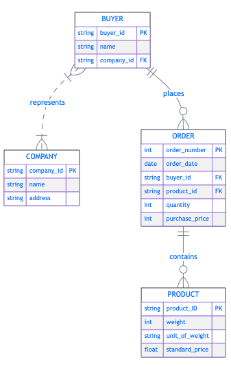
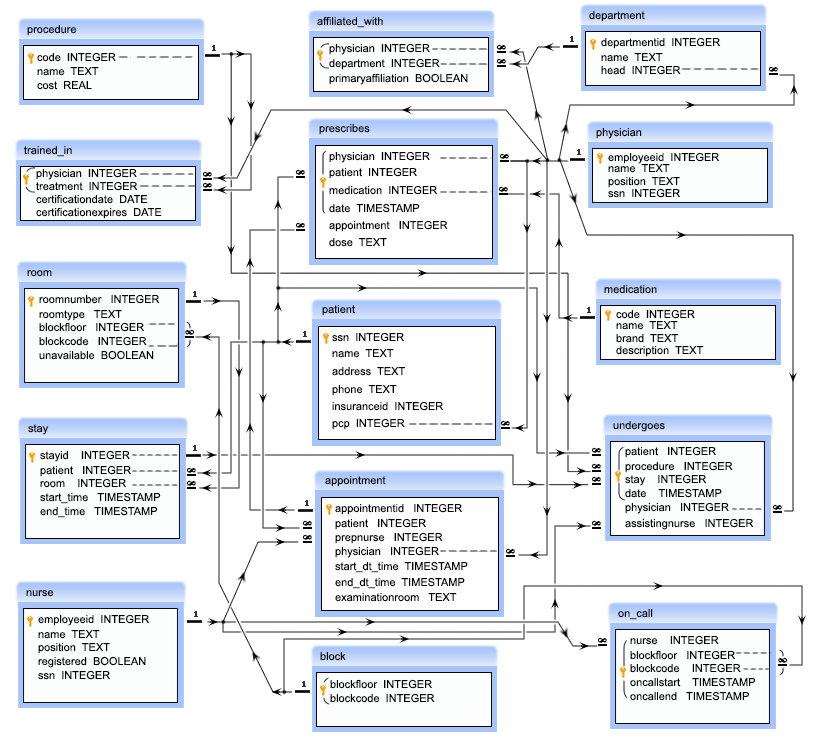
Figure 8.2 shows a different style of E-R diagram commonly used for database schema. The arrows link individual fields as primary and foreign keys for the tables and show the type of the relationships.

Figure 8.2: A partial E-R diagram from a hospital setting. w3resource (2023)

8.3.4 Bringing Tables Together

Now that we can see the database schema, we can find where the data is that we want.

Suppose we want to answer the question, how many orders were placed in the last month. We can do that with just the data in the ORDERS table.

However, suppose we want to answer the question how many orders were placed from buyers in the states of Virginia and Maryland last month. We would have to get data from both the ORDERS table and the BUYERS table.

We get data from multiple tables by temporarily combining tables using a SQL query that creates a JOIN between two or more tables.

Database joins are the same joins you can execute using {dplyr} verbs but the SQL syntax is slight different.

If you are using the same join over and over in your analysis. SQL allows you to create a database “View” and save it. Then in the future, you can query the “view” instead of having to rejoin the tables.

• This is analogous to writing an R function to create a data frame based on joins and querying the results of the function instead of rewriting the code to join the data frames.

8.3.5 Query Optimization in Database Systems

Database Management Systems (DBMS) do more than store data and execute queries, they also decide how to execute your query.

This process is known as query optimization.

When you write a SQL statement,

• You describe what result you want
• The database engine determines how to retrieve it efficiently.

8.3.5.1 Table Scans vs. Index Lookups

At the most basic level, the database has two broad strategies for locating rows:

• Table Scan (Sequential Scan)
  • The database reads each row (or each relevant column in a columnar system) and checks whether it satisfies the condition.
  • This is simple and reliable but can be expensive for large tables.
• Index Lookup
  • If an index exists on a column used in a WHERE, JOIN, or ORDER BY clause, the database can use that index to jump directly to matching rows instead of scanning the entire table.

Conceptually, an index acts like a pre-built mapping so it knows:

'JFK' → rows 1, 15, 208, 9042, ...
'LGA' → rows 2, 19, 203, ...

Instead of checking every row to find origin = 'JFK', the engine can navigate directly to the relevant row locations.

Most databases automatically create indexes for:

• The PRIMARY KEY for each table.
• UNIQUEness constraints the designer imposes on a table

Additional indexes must be created explicitly using:

CREATE INDEX idx_column
ON table_name(column_name);

8.3.5.2 How the Optimizer Chooses

Modern RDBMS use a “cost-based” query optimizer.

• Cost is not about dollars, it is a statistical estimate of system effort.

That effort is primarily measured in terms of:

• Disk I/O (reading and writing data): usually the most “expensive”
• Memory usage: certain queries require large working memory.
• CPU operations: more rows –> more CPU cycles.
• Network transfer: more rows/columns = more bytes transmitted to the front-end client
• Temporary storage usage
• Concurrency impact

The optimizer chooses the plan with the lowest estimated total resource usage.

The optimizer evaluates:

• Table size
• Available indexes
• Estimated number of matching rows
• Join cardinality, e.g., one-to-one, one-to-many, etc.
• [Memory availability]

It then chooses the execution plan with the “lowest estimated cost (resource usage).”

• Importantly: Using an index is not always optimal.
• If a large percentage of rows match a condition, scanning the table may be faster than using the index.

8.3.5.3 Analytical vs. Transactional Systems

In transactional (row-based) systems:

• Users typically use queries focused on retrieving a small numbers of rows.
• Indexes are critical for fast point look-ups.

In analytical (columnar) systems like DuckDB:

• Users often use queries focused on retrieving many rows.
• Thus the DBMS has optimized how it does Full column scans.
• Selecting fewer columns reduces I/O dramatically.
• Indexes are less central than in traditional OLTP systems.

Understanding this distinction explains why some queries scan entire tables and why that is not necessarily bad in an analytical (columnar) database.

8.3.5.4 Why This Matters

Knowing that databases choose between scans and index lookups helps explain:

• Why filtering early improves performance.
• Why SELECT * increases input and output “costs” (I/O).
• Why large joins can become slow.
• Why ORDER BY and GROUP BY can require additional memory and sorting.

You do not need to design execution plans manually, but understanding that the database is optimizing behind the scenes makes you a more effective SQL user.

8.3.6 Database Design

Designing databases is its own area of expertise.

A poorly designed database will be slow and have insufficient rules (safeguards) to ensure data integrity.

We are used to operating as single users of our data since it is all in the memory of our machine and we can do what we want.

• A database may have thousands of users at the same time trying to update or retrieve records.
• Only one user can update a record at a time so databases use Record Locking to prevent others from updating the record or even retrieving it while someone else is updating the record.
• RDBMS can enforce locking at higher levels such as the table or even the entire database which can delay user queries. See All about locking in SQL Server for more details.

Database designers make trade offs when designing tables to balance competing desires.

• Storage Efficiency: limit each table to a single entity to minimize the amount of redundant data. This can generate lots of tables.
• Maintenance Efficiency: The more tables you have, the fewer users might be trying to update the table at a time.
• Query Speed: Minimize the number of joins needed to make a query. This leads to fewer tables.

These trade offs were recognized by Codd in his original paper.

• Formal descriptions of the ways to design databases are known as Normal forms.
• The process for determining what form is best for an application is known as Database Normalization. For more info see The Trade-offs Between Database Normalization and Denormalization. Explorer (2023)

Thus database designers may create tables that have redundant data if the most common queries join fields from those tables.

They will use database performance testing to optimize the queries and the database design to get the optimal cost performance trade offs. They can use other approaches to support data integrity in addition to database normalization.

Don’t be surprised to see E-R diagrams that have redundant data in them.

Database Partitions

In very large databases, designers often choose to physically partition tables, e.g., by month or year. This only affects how the data is stored, not the logical relationships between tables.

• This is not the same construct as the PARTITION BY clause in Section 8.19.

• When a query filters on the partition column, the database can skip entire partitions (a process called partition pruning), dramatically improving performance.

• This affects speed and (in cloud systems) cost, but not the correctness of results.

Partitioning does not change:

• SQL syntax
• Query logic
• Result correctness

It only changes how efficiently the engine executes the query.

8.3.7 Relational Database Management Systems

8.3.7.1 Database Front and Back Ends

Databases have two main components.

• The Front-end user interface where users create code to generate queries and receive results.
• The Back-end server where the data is stored and the DBMS executes the queries to update or retrieve the data.

The Front-end and Back-end communicate through a Connection that uses an API for handling queries and data.

Many RDBMS bundle a Front-end and Back-end together. Examples include Oracle, SAP, and DuckDB has DBeaver.

Most databases allow you to use a Front-end of your choice as long as you have a server driver you can use to configure and open a connection to the Back-end server of the database.

• RStudio can operate as a Front-end to RDBMS for which you have installed a server.
• Excel can operate as a Front-end to a Microsoft SQL Server database.
• DBeaver allows you to make a connection to many different DBMS servers.
• MariaDB identifies over 30 Front-ends that can work with it, including DuckDB’s DBeaver SQL IDE.

There are multiple solutions. We can use RStudio, Positron, DBeaver, or other IDEs.

8.3.7.2 Database Connections: ODBC and the {DBI} Package

The reason there is so much flexibility with connecting Front and Back ends is the standardization of the Microsoft Open Data Base Connectivity (ODBC) Standard. David-Engel (2023)

The ODBC standard was designed for “maximum interoperability”.

The construct is similar to the HTTP interface for web browsers. The DBMS developer creates a driver that serves as an API for their Back-end DBMS that is ODBC-compliant. Then the Front-end developer creates their software to also be ODBC-compliant.

That way, the Front-end can create a connection to and interact with any DBMS back end for which there is an ODBC-compliant driver.

The R {DBI} package (for Data Base Interface) supports the connection between R and over 25 different DBMS Back-ends.

• Popular Back-end packages include: {duckdb}, {RMariaDB}, {RPostgres}, {RSQLite}, and {bigrquery}.
• These packages include the ODBC-compliant driver for the given database.

If no one has written a package but an ODBC-compliant driver exists, the {DBI} package works with the {ODBC} package and the driver to make the connection to the Back-end server.

8.3.7.3 Database Configuration Types

RDBMS can also be categorized based on their configuration or how front and back ends are physically connected and how the data is stored.

• In-process databases run on your computer. The data is stored locally and accessible without a network connection.
  • They are optimized for the use case of a single user working with large amounts of data.
• Client-Server databases use a small front-end client on your computer (perhaps an IDE or in a browser) to connect to a robust server over a network. Data can be stored across a set of servers.
  • They are optimized for the use case where multiple users can query the database at once and the RDBMS resolves contention.
• Cloud-databases also separate the front and back ends over a network but now the data may be distributed across multiple locations in the cloud.
  • These are optimized for the use case of multiple users accessing a wide-variety of very large data and enabling distributed computing and parallel computing.

With the proliferation of cloud computing and software as a service (SAAS), you can expect to see more and more hybrids of client server and cloud databases.

As the amount of collected structured and unstructured data scales to Apache solutions for “Big Data”, the fundamental concepts of exploiting relationships in data using some version of SQL will continue to apply for the foreseeable future.

8.4 SQL Basics

We will use R Studio as the Front-end, DuckDB as the Back-end, and the {DBI} package to support the connection between the front and back ends.

8.4.1 Connecting to a Database

Before you can use SQL to interact with a database, you must have a way to connect the Front-end user interface to the Back-end server with the data.

• When working in R, the {DBI} package can create the connection and allow you to assign a name to it.
• Your database will be created by a specific DBMS which provides the Back-end server.
• If you are not using the Front-End that comes with the DBMS, you need an ODBC-compliant driver for the DBMS to make the connection.

We will use the DuckDB database and the {duckdb} Package for most of this section.

• DuckDB is an in-process database so it has no external dependencies which makes it useful for single user analysis of large data. See Why DuckDB for their story.

• You can install DuckDB directly on your computer and use the built-in Command Line Interface without using R.

• However, the {duckdb} package installs the DuckDB DBMS as well as the ODBC-compliant driver for R.

• Use the console to install {DBI} and {duckdb}.

To make the connection between R and DuckDB requires loading the two packages {DBI} and {duckdb}.

library(DBI)
library(duckdb)

We also want to compare the SQL code (working with the database tables) with R code (working with data frames) so load {tidyverse} and {nycflights13} which has the same data as the database we will use.

• You will see the concepts for accessing data are quite similar but the syntax is different.

library(nycflights13)
library(tidyverse)

The DuckDB database with {nycflights13} data is on GitHub at https://github.com/AU-datascience/data/blob/main/413-613/flights.duckdb.

Important

• {duckdb} only works with local data bases, not over a URL

• You can manually download to a data folder under your current file’s working directory or use the following once you are sure there is a data directory:

# GitHub raw link for the DuckDB database file
url <- "https://github.com/AU-datascience/data/raw/main/413-613/flights.duckdb"

# Local path to save the file
dest <- here("data", "flights.duckdb")

# Download the file
download.file(url, dest, mode = "wb")

Create a connection to flights.duckdb by using DBI::dbConnect() with duckdb() and a relative path to the database and assign the name con to the connection.

con <- dbConnect(duckdb(dbdir = "./data/flights.duckdb"))
class(con)

[1] "duckdb_connection"
attr(,"package")
[1] "duckdb"

• Notice the connection to the database in the environment.
• You will use the con connection to interact with the database Back-end.

Important

• When using DuckDB through DBI,
  • SQL runs in the database
  • Results are pulled into R only when requested
  • dbGetQuery() materializes the results into memory

Once you have a connection, you can create a basic SQL code chunk like this in R Markdown.

```{sql, connection=con}
--| label: lst-show-tables
-- [SQL:DuckDB] SHOW TABLES is not part of the SQL standard.
SHOW TABLES;
```

5 records

name
airlines
airports
flights
planes
weather

In Quarto .qmd files use the chunk option --| connection: con.

```{sql}
--| connection: con
--| label: lst-show-tables-q
-- [SQL:DuckDB] SHOW TABLES is not part of the SQL standard.
SHOW TABLES;
```

5 records

name
airlines
airports
flights
planes
weather

Important

Whenever you are using a SQL chunk inside an R Markdown or Quarto document, identify the connection in each code chunk so the SQL interpreter knows with which database to interact.

All the SQL code chunks in this section will have the --| connection my_con chunk option where my_con is the name of the appropriate connection.

8.4.2 Connecting to Parquet Files

DuckDB and other modern databases (e.g., Apache Spark, Presto/Trino, Google BigQuery, Snowflake, Databricks) explicitly support the reading and writing of Parquet files.

• Parquet is extremely common today in big data and analytics; it’s basically the default format for modern data lakes and replacing CSV as a format for data exchange.
• Parquet is a columnar, compressed, self-describing format so systems built with columnar execution in mind (analytics DBs, OLAP engines, distributed query engines) tend to support direct querying of compressed Parquet.
• Traditional RDBMS (Postgres, MySQL, SQL Server, Oracle) may require an extension or pre-processing to ingest them.

Note

Parquet is a storage format, not a relational database.

• It preserves schema information (column names, types, and optional metadata).
• It does not preserve or enforce higher-level relational rules such as: Primary keys, Foreign keys, Indexes, or Constraints (NOT NULL, CHECK, etc.).

In parquet format, each table can be a separate file or a set of files (for really large data).

• The files can be compressed for efficient storage.

Assume there is a directory (“./data/parquet”) of tables where each file is a separate table

• Create a new connection.
• Read individual files by name.

con_p <- dbConnect(duckdb())

• DESCRIBE a table.

```{sql}
--| connection: con_p
--| label: lst-read_parquet
-- [SQL:DuckDB] DESCRIBE 'file.parquet' treats a file path as a table-like object.
DESCRIBE  './data/parquet/flights.parquet';
```

Displaying records 1 - 10

column_name	column_type	null	key	default	extra
year	INTEGER	YES	NA	NA	NA
month	INTEGER	YES	NA	NA	NA
day	INTEGER	YES	NA	NA	NA
dep_time	INTEGER	YES	NA	NA	NA
sched_dep_time	INTEGER	YES	NA	NA	NA
dep_delay	DOUBLE	YES	NA	NA	NA
arr_time	INTEGER	YES	NA	NA	NA
sched_arr_time	INTEGER	YES	NA	NA	NA
arr_delay	DOUBLE	YES	NA	NA	NA
carrier	VARCHAR	YES	NA	NA	NA

When you have a DuckDB connection (here called con_p), DuckDB can automatically treat Parquet file paths as virtual tables so you can work with them.

• Here is an example of a JOIN of two parquet files. (Don’t worry about the syntax for now.)

```{sql}
--| connection: con_p
--| label: lst-join_parquet
-- [SQL:DuckDB] DuckDB can query Parquet files by path in FROM/JOIN (non-standard).
SELECT f.flight, a.name AS airline_name
FROM './data/parquet/flights.parquet' AS f
JOIN './data/parquet/airlines.parquet' AS a
  ON f.carrier = a.carrier
LIMIT 10;
```

Displaying records 1 - 10

flight	airline_name
461	Delta Air Lines Inc.
569	United Air Lines Inc.
4424	ExpressJet Airlines Inc.
6177	ExpressJet Airlines Inc.
731	Delta Air Lines Inc.
684	United Air Lines Inc.
301	American Airlines Inc.
1837	American Airlines Inc.
1279	Delta Air Lines Inc.
1691	United Air Lines Inc.

Using the file names directly though makes the code less portable and harder to read.

To make portable code, create a VIEW for each table (Section 8.25) with an alias of the table name and write your code using the VIEW instead of the file name as working with a DBMS table.

• Let’s close the con_p connection

dbDisconnect(con_p)

• Use R to create a new connection and the views.

# create connection (here, ephemeral in-memory db)
con_p <- dbConnect(duckdb())

# register all Parquet files in a folder
dbExecute(con_p, "
  CREATE VIEW flights AS
  SELECT * FROM parquet_scan('./data/parquet/flights.parquet');

  CREATE VIEW airlines AS
  SELECT * FROM parquet_scan('./data/parquet/airlines.parquet');
")

[1] 0

Now we can use the new connection to run the query as if it were standard SQL.

```{sql}
--| connection: con_p
--| label: lst-join_parquet-view
-- [SQL:Mostly standard] This becomes portable once you hide Parquet behind views.
SELECT f.flight, a.name AS airline_name
FROM flights AS f
JOIN airlines AS a
  ON f.carrier = a.carrier
LIMIT 10;
```

Displaying records 1 - 10

flight	airline_name
67	United Air Lines Inc.
373	JetBlue Airways
764	United Air Lines Inc.
2044	Delta Air Lines Inc.
2171	US Airways Inc.
1275	Delta Air Lines Inc.
366	Southwest Airlines Co.
1550	United Air Lines Inc.
4694	ExpressJet Airlines Inc.
1647	Delta Air Lines Inc.

• Close the connection

dbDisconnect(con_p)

8.4.3 SQL Syntax Overview

Like all languages, SQL has standard syntax and reserved words.

However, SQL is declarative, not procedural in that it describes what result you want, not how to compute it.

Important

There is a standard for SQL: SQL-92. However, many database developers see this as a point of departure rather than a destination.

• They use ODBC and SQL-92 to develop their own versions that are optimized for their intended use cases and database design.
• Thus, there are many flavors of SQL in the world.

Be sure to review the SQL implementation for the DBMS you are using to be aware of any special features.

If you use proprietary SQL, it may give you performance improvements, but it will also lock you into that DBMS and you will have to revise your code if the back-end DBMS is changed.

These notes use the SQL flavor used by the DuckDB DBMS.

The Tidyverse uses functions as “verbs” to manipulate data; SQL uses “STATEMENTS” which can contain clauses, expressions, and other syntactic building blocks.

Table 8.1 identifies the common types of building blocks used in SQL along with some examples and their usage.

Table 8.1: SQL Language Building Blocks

Type	Examples	Role / Purpose
Statements	SELECT, INSERT, UPDATE, DELETE, CREATE, DROP	Complete SQL commands that tell the database what action to perform.
Clauses	FROM, WHERE, GROUP BY, HAVING, ORDER BY, LIMIT, JOIN	Sub-components of statements that define how the action is carried out.
Expressions	CASE, arithmetic (a + b), boolean (x > 5), string concatenation	Return a single value, often used inside clauses (computed or conditional).
Functions	Aggregate: SUM(), AVG(), COUNT() Scalar: ROUND(), UPPER(), NOW()	Built-in operations that transform values or sets of values.
Modifiers	DISTINCT, ALL, TOP, AS (alias)	Adjust or qualify the behavior of clauses or expressions.
Predicates	IN, BETWEEN, LIKE, IS NULL, EXISTS	Conditions that return TRUE/FALSE, often used in WHERE or HAVING.
Operators	=, <, >, AND, OR, NOT, +, -, *, /	Combine or compare values.
Keywords	NULL, PRIMARY KEY, FOREIGN KEY, DEFAULT, CHECK	Special reserved words that define schema rules or literal values.

A SQL “statement” is a “complete sentence” that can be executed independently as an executable query.

• A clause is a phrase in the sentence.
• An expression is like a formula inside a clause.
• A function is a built-in calculator you can call inside expressions.
• Modifiers tweak the behavior (like adverbs in English).
• Predicates make true/false checks.
• Operators are the glue (math or logic).
• Keywords are the reserved words that give SQL its grammar.

The following diagram shows how the building blocks are ordered in creating a complete sentence.

--| label: lst-sql-sequence
--| lst-cap: Generalized hierarchy of SQL building blocks
--| echo: true
SQL Statement (e.g., SELECT)
│
├── Clauses (parts of the statement)
│   ├── FROM (which tables?)
│   ├── WHERE (filter rows before grouping)
│   │   └── Predicates (IN, BETWEEN, LIKE, IS NULL, EXISTS)
│   │       └── Expressions (x > 5, col1 + col2)
│   ├── GROUP BY (form groups)
│   ├── HAVING (filter groups after aggregation)
│   │   └── Aggregate Functions (SUM, AVG, COUNT, MIN, MAX)
│   ├── SELECT (choose fields/expressions to return)
│   │   ├── Expressions (CASE, arithmetic, concatenation)
│   │   │   └── Functions (ROUND, UPPER, NOW, SQRT, etc.)
│   │   └── Modifiers (DISTINCT, AS alias)
│   ├── ORDER BY (sort results)
│   └── LIMIT / OFFSET (restrict result size)
│
├── Operators (math: +, -, *, / ; logic: AND, OR, NOT ; comparison: =, <, >)
│
└── Keywords (NULL, DEFAULT, PRIMARY KEY, FOREIGN KEY, CHECK, etc.)

SQL is used across the entire database workflow:

• Database setup: CREATE DATABASE, CREATE TABLE
• Data management: INSERT, UPDATE, DELETE, DROP TABLE, ALTER TABLE
• Data retrieval and analysis: SELECT (with various clauses)

We are most interested in SELECT statements as that is how we get data from a database table or a set of joined tables.

8.4.4 The SELECT statement

The SELECT statement is the SQL workhorse for getting and manipulating data akin to dplyr::select() combined with filter(), arrange(), and summarise().

SELECT has several other clauses or keywords to support tailoring the data returned by a query.

• FROM: Required to identify the table or set of tables where the data will be located.
• WHERE is a clause used to filter which records (rows) should be returned like dplyr::filter().
• ORDER BY is a keyword for sorting records like dplyr::arrange(). The default is ascending order.
• GROUP BY is a keyword akin to dplyr::group_by and is used for creating summaries of data, often with aggregate functions (SUM(), AVG(), COUNT(), …).

Other useful modifiers include:

• AS: rename/alias columns or tables (like dplyr::rename()).
• IN: test membership (like %in%).
• DISTINCT: removes duplicate rows (like dplyr::distinct()).
• LIMIT: restrict number of rows returned (like utils::head()).

SELECT Statement Operators

• SQL uses = for comparison instead of == since you don’t assign anything in SQL.
• Use != for not equal.
• SQL uses NULL instead of NA. Test with IS NULL or IS NOT NULL.
• SQL uses AND, OR and NOT as logical operators.

8.4.5 SQL Syntax Rules to Remember

1. Case Insensitivity:

• Keywords are case insensitive, i.e. select is the same as SELECT is the same as SeLeCt).
• Best practice is to have all statement keywords be in UPPERCASE (e.g., SELECT) and table/field names in lowercase for readability.

2. Order Matters:
   

• A SQL SELECT statement’s clauses and keywords must be in the following order: SELECT, FROM, WHERE, GROUP BY, ORDER BY.

3. Whitespace and Formatting:
   

• SQL ignores newlines and extra spaces.
• Best practice is to put statements, clauses, and keywords on new lines with spaces to align the keywords to preserve a “river” of white space between the keyword and the values.

4. Quoting Rules:

• Character string values must be in single quotes, e.g., 'NYC'.
• Identifiers (column/table names): use double quotes (“first name”) if they contain spaces, reserved words, or special characters (same as using back ticks in R).
• It is fine to always use double quotes because it is not always clear what is an invalid variable name in the database management system.

5. Comments

• Single-line comments start with two hyphens --.
• Multi-line comments use /* ... */ in most DBMS.

6. Statement Termination

• Some databases (e.g., PostgreSQL, Oracle) require a semicolon ; at the end of each statement.
• Best practice is to always include ; so multiple statements can be run in one batch.

7. Three-valued Logic

• Unlike R or Python, SQL uses three-valued logic as expressions can evaluate to:
  • TRUE,
    • FALSE, or
    • UNKNOWN (when NULL is involved)
  • NULL does not mean zero or empty string. It means missing or unknown.
• This affects comparisons, e.g. the following always returns UNKNOWN not TRUE.

SELECT *
FROM flights
WHERE arr_delay = NULL;   -- This will NOT work

• The correct approach is

WHERE arr_delay IS NULL;
WHERE arr_delay IS NOT NULL;

• NULL = NULL is UNKNOWN, not TRUE.
  • WHERE only keeps rows where the condition evaluates to TRUE.
  • FALSE and UNKNOWN rows are both filtered out.
• SQL is forgiving about formatting, but unforgiving about logic, especially with NULL handling.

Together, these rules make SQL predictable (rigid order) but also forgiving (case, whitespace, optional semicolons).

8.4.6 Creating SQL Code Chunks

If you are creating working a lot with SQL in RStudio, you can manually enter a chunk and change the language engine to sql each time. However there are other ways to be more productive.

8.4.6.1 Customize a Keyboard Shortcut

RStudio has a built-in capability to create an SQL code chunk with an R Markdown code chunk option for the connection.

To access it quickly, suggest customizing a keyboard shortcut for it per Customizing Keyboard Shortcuts in the RStudio IDE. Ushey (2023)

Go to the RStudio Main Menu and select Tools/Modify Keyboard Shortcuts.

• A pop up pane will appear with many options and the existing keyboard shortcuts.
• Enter S Q in the search pane and you should see something like Figure 8.3.

Figure 8.3: A custom keyboard shortcut for an SQL code chunk.

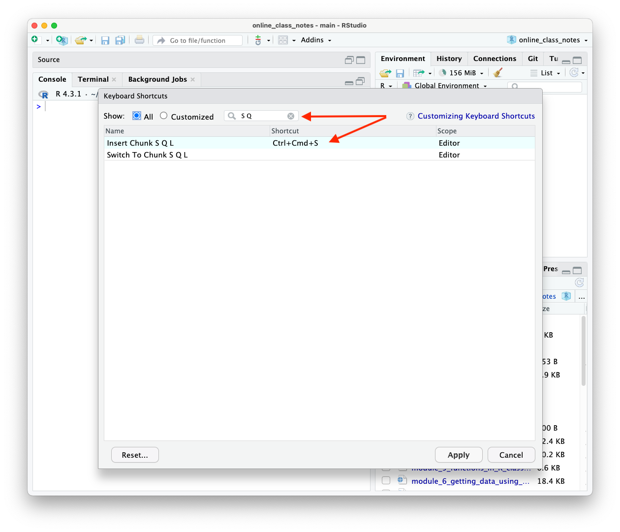
• Click in the Shortcut column to the right of “Insert Chunk S Q L”.
• Enter the shortcut combination you want. Figure 8.3 shows the Mac shortcut I chose, Ctrl + Cmd + s.
• Click Apply and your shortcut will be saved. You can use it right away.

Enter the shortcut in a text area (not an existing chunk) and you should get the following (without the con).

• Make sure you enter in the name of the connection you have created.

```{sql connection=con}

```

Important

• You cannot render a document with an SQL code chunk with invalid or empty connection.
• You have to have created a valid connection object before the SQL code chunk.
• If you have a connection, you must also have a valid SQL line, or set the code chunk option --| eval: false.

8.4.6.2 Create a Custom Code Snippet

Another option in RStudio is to create a custom code snippet per Code Snippets in the RStudio IDE. Allaire (2023)

• RStudio snippets are templates for code or R Markdown.

To create a snippet for a custom SQL code chunk, go to the RStudio Main Menu and select Tools/Edit Code Snippets.

• A pop-up pane should appear.
• Select Markdown as you will be using the snippet in a Markdown text section.
• You will see something like Figure 8.4 with the existing Markdown code snippets.

Figure 8.4: A Markdown code snippet for an SQL code chunk.

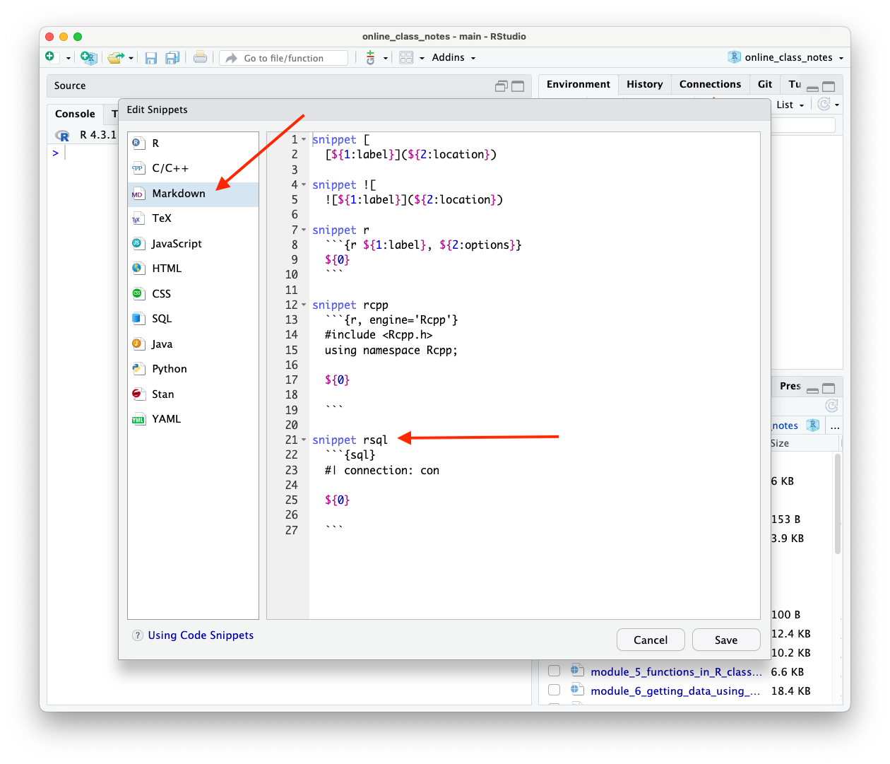
• Figure 8.4 already shows the snippet I saved for creating a custom SSQL code chunk.

You can create your own snippet.

• Enter snippet s_name where you enter your name for the snippet instead of s_name. It does not have to be rsql.
• Enter the following lines and use the tab key not spaces to indent.
• The ${0} is a placeholder for your SQL code. The 0 means it is the first place your cursor will go.
  • You could replace con with ${0} so you can fill in which connection each time. Then edit the next ${0} on the original line to ${1}.
• Select Save to save it and then you can use it.

To use a snippet, enter the name your created, I use “rsql”, and then SHIFT+TAB (on a mac) aTAB on windows, and the code chunk will appear like below (without the other options).

```{sql}

```

8.5 A SQL-R-Python Mental Model

Part of being a “tri-lingual” data scientist is moving fluently between SQL, R, and Python.

Doing so efficiently requires more than translating syntax; it requires mapping the underlying mental models of how each language stores, processes, and returns data.

• A key idea is SQL describes the result; R and Python describe the steps.

Table 8.2 provides a concise comparison to help translate core concepts across these three common data science environments.

Table 8.2: SQL concepts compared to similar concepts in R and Python

Concept	SQL	R	Python (pandas)
Fundamental object	Table (relation)	Data frame / tibble	DataFrame
Storage model	Often disk-based	In-memory	In-memory
Where execution happens	In the database engine	In R session memory	In Python process memory
Evaluation style	Declarative (describe result)	Functional / vectorized	Method chaining / vectorized
Execution model	Set-based (engine optimized)	Vectorized in memory	Vectorized in memory
Optimization responsibility	Database optimizer chooses plan	User controls order of operations	User controls order of operations
Query result	Always returns a new table	Returns object (vector/data frame)	Returns DataFrame/Series
Pipelining model	Nested queries / CTEs	Pipe (|>)	Method chaining (.)
Row order	Not guaranteed unless ORDER BY	Preserved unless changed	Preserved unless changed
Missing values	NULL (three-valued logic)	NA	NaN / None
Test for missing	IS NULL	is.na()	.isna()
Filtering behavior	WHERE keeps only TRUE	Logical vector keeps TRUE	Boolean mask keeps True
Joins	Explicit JOIN syntax	*_join() functions	merge() / .join()
Arithmetic behavior	Depends on type (integer vs numeric)	Numeric by default	Numeric by default

A mental model helps in seeing that the analytical thinking remains the same; only the execution model changes across SQL, R, and Python.

Now we are ready to go through a number of the SQL Building blocks from Table 8.1 to manipulate and retrieve data using the connection to our DuckDB database.

Since there are many flavors of SQL, and almost every flavor (including DuckDB) uses some non-standard statements or functions, the SQL chunks in this section are annotated as follows to indicate what is standard in DuckDB, what is customized in the DuckDB flavor and what is “mostly standard”.

• -- [SQL:Standard] = should run on most DBMS (with minor naming differences)
• -- [SQL:DuckDB] = DuckDB feature or commonly-nonportable syntax
• -- [SQL:Mostly standard; note …] = portable core + one portability caveat

8.6 SHOW and DESCRIBE Provide an Overview of the Tables in the Database

DuckDB’s SHOW TABLES returns a list of all of the tables in the database.

```{sql}
--| connection: con
--| label: lst-show-tables-3
-- [SQL:DuckDB] SHOW TABLES is not part of the SQL standard.
-- List all tables in the database
SHOW TABLES;
```

5 records

name
airlines
airports
flights
planes
weather

DESCRIBE tablename returns metadata about the table tablename.

• column name, data type, whether NULL is allowed, key info (e.g. primary key), default values.

```{sql}
--| connection: con
--| label: lst-describe-table-airlines
-- [SQL:DuckDB] DESCRIBE table is supported in DuckDB; many DBMS use information_schema instead.
-- Structure of a specific table
DESCRIBE airlines;
```

2 records

column_name	column_type	null	key	default	extra
carrier	VARCHAR	YES	NA	NA	NA
name	VARCHAR	YES	NA	NA	NA

• R equivalents for a data frame

str(flights)

tibble [336,776 × 19] (S3: tbl_df/tbl/data.frame)
 $ year          : int [1:336776] 2013 2013 2013 2013 2013 2013 2013 2013 2013 2013 ...
 $ month         : int [1:336776] 1 1 1 1 1 1 1 1 1 1 ...
 $ day           : int [1:336776] 1 1 1 1 1 1 1 1 1 1 ...
 $ dep_time      : int [1:336776] 517 533 542 544 554 554 555 557 557 558 ...
 $ sched_dep_time: int [1:336776] 515 529 540 545 600 558 600 600 600 600 ...
 $ dep_delay     : num [1:336776] 2 4 2 -1 -6 -4 -5 -3 -3 -2 ...
 $ arr_time      : int [1:336776] 830 850 923 1004 812 740 913 709 838 753 ...
 $ sched_arr_time: int [1:336776] 819 830 850 1022 837 728 854 723 846 745 ...
 $ arr_delay     : num [1:336776] 11 20 33 -18 -25 12 19 -14 -8 8 ...
 $ carrier       : chr [1:336776] "UA" "UA" "AA" "B6" ...
 $ flight        : int [1:336776] 1545 1714 1141 725 461 1696 507 5708 79 301 ...
 $ tailnum       : chr [1:336776] "N14228" "N24211" "N619AA" "N804JB" ...
 $ origin        : chr [1:336776] "EWR" "LGA" "JFK" "JFK" ...
 $ dest          : chr [1:336776] "IAH" "IAH" "MIA" "BQN" ...
 $ air_time      : num [1:336776] 227 227 160 183 116 150 158 53 140 138 ...
 $ distance      : num [1:336776] 1400 1416 1089 1576 762 ...
 $ hour          : num [1:336776] 5 5 5 5 6 5 6 6 6 6 ...
 $ minute        : num [1:336776] 15 29 40 45 0 58 0 0 0 0 ...
 $ time_hour     : POSIXct[1:336776], format: "2013-01-01 05:00:00" "2013-01-01 05:00:00" ...

glimpse(flights)

Rows: 336,776
Columns: 19
$ year           <int> 2013, 2013, 2013, 2013, 2013, 2013, 2013, 2013, 2013, 2…
$ month          <int> 1, 1, 1, 1, 1, 1, 1, 1, 1, 1, 1, 1, 1, 1, 1, 1, 1, 1, 1…
$ day            <int> 1, 1, 1, 1, 1, 1, 1, 1, 1, 1, 1, 1, 1, 1, 1, 1, 1, 1, 1…
$ dep_time       <int> 517, 533, 542, 544, 554, 554, 555, 557, 557, 558, 558, …
$ sched_dep_time <int> 515, 529, 540, 545, 600, 558, 600, 600, 600, 600, 600, …
$ dep_delay      <dbl> 2, 4, 2, -1, -6, -4, -5, -3, -3, -2, -2, -2, -2, -2, -1…
$ arr_time       <int> 830, 850, 923, 1004, 812, 740, 913, 709, 838, 753, 849,…
$ sched_arr_time <int> 819, 830, 850, 1022, 837, 728, 854, 723, 846, 745, 851,…
$ arr_delay      <dbl> 11, 20, 33, -18, -25, 12, 19, -14, -8, 8, -2, -3, 7, -1…
$ carrier        <chr> "UA", "UA", "AA", "B6", "DL", "UA", "B6", "EV", "B6", "…
$ flight         <int> 1545, 1714, 1141, 725, 461, 1696, 507, 5708, 79, 301, 4…
$ tailnum        <chr> "N14228", "N24211", "N619AA", "N804JB", "N668DN", "N394…
$ origin         <chr> "EWR", "LGA", "JFK", "JFK", "LGA", "EWR", "EWR", "LGA",…
$ dest           <chr> "IAH", "IAH", "MIA", "BQN", "ATL", "ORD", "FLL", "IAD",…
$ air_time       <dbl> 227, 227, 160, 183, 116, 150, 158, 53, 140, 138, 149, 1…
$ distance       <dbl> 1400, 1416, 1089, 1576, 762, 719, 1065, 229, 944, 733, …
$ hour           <dbl> 5, 5, 5, 5, 6, 5, 6, 6, 6, 6, 6, 6, 6, 6, 6, 5, 6, 6, 6…
$ minute         <dbl> 15, 29, 40, 45, 0, 58, 0, 0, 0, 0, 0, 0, 0, 0, 0, 59, 0…
$ time_hour      <dttm> 2013-01-01 05:00:00, 2013-01-01 05:00:00, 2013-01-01 0…

Note

• DuckDB has a non-standard version of DESCRIBE, without a table name, where it returns the set of tables with columns for the table names, their column names, and column types.

```{sql}
--| connection: con
--| label: lst-describe-table
--| eval: false
-- [SQL:DuckDB] DuckDB-only: DESCRIBE with no table name.
DESCRIBE;
```

8.7 SELECT Can Return Specific Fields (columns) FROM a Table

• In most data retrieval queries, the SELECT statement is followed by a FROM clause which identifies the source of the data.
  • That source is a table, a set of joined tables, or a previously-created table view (a saved query like an intermediate data frame variable).
• The data which is returned as a result of executing a SELECT statement is stored in a result table, which can also be called the result-set.
  • This means you can use the output as a table in a new FROM clause.
• A SELECT statement can have other clauses and modifiers to reduce the amount of data that is returned.
• There is no equivalent for excluding fields (like dplyr::select(-year)). Just select the fields you want.

```{sql}
--| eval: false
--| connection: con
-- [SQL:Standard] Building-block examples are standard SQL constructs (names vary by DBMS)
SELECT <field1>, <field2>, <field3> 
FROM <mytable>;
```

Let’s use this syntax to get all the data in the fields tailnum, year, and model from the planes table.

```{sql}
--| connection: con
--| label: lst-select-planes
-- [SQL:Standard] Quoting identifiers with double-quotes is standard SQL, 
-- but not all DBMS default to it.
SELECT "tailnum", "year", "model" 
FROM planes;
```

Displaying records 1 - 10

tailnum	year	model
N10156	2004	EMB-145XR
N102UW	1998	A320-214
N103US	1999	A320-214
N104UW	1999	A320-214
N10575	2002	EMB-145LR
N105UW	1999	A320-214
N107US	1999	A320-214
N108UW	1999	A320-214
N109UW	1999	A320-214
N110UW	1999	A320-214

• R equivalent

planes |>
  select(tailnum, year, model)

Think of SELECT ... FROM ... as the core skeleton of every SQL query.

• Everything else (WHERE, GROUP BY, ORDER BY, etc.) adds constraints to shape the result-set, typically to be fewer rows that more focused on the data needed for the question at hand.

8.7.1 SELECT without a FROM

SQL SELECT can do more than retrieving columns from tables; it is the mechanism for evaluating expressions and returning result sets.

• Even when no table is referenced (there is no FROM), SELECT returns a one-row result table containing the computed value(s).

This can be useful for:

• Quick calculations
• Testing functions
• Checking database connectivity
• Inspecting system metadata

8.7.1.1 SELECT as a calculator

• This is often used interactively while developing more complex queries.

```{sql}
--| connection: con
-- [SQL:Standard] Simple expression; portable.
SELECT 100 * 0.08;
```

1 records

(100 * 0.08)
8

```{sql}
--| connection: con
-- [SQL:Mostly standard; note POWER()] POWER() exists in many DBMS; 
-- a few use different names (e.g., POW()).
SELECT POWER(2, 10);
```

1 records

power(2, 10)
1024

```{sql}
--| connection: con
-- [SQL:Standard] CAST is portable.
SELECT CAST(5 AS DOUBLE) / 2;
```

1 records

(CAST(5 AS DOUBLE) / 2)
2.5

8.7.1.2 Using SELECT to Check connectivity

• SELECT 1; is commonly used by applications and connection pools to verify the database connection is alive.
  • It requires no tables and executes quickly.

```{sql}
--| connection: con
-- [SQL:Standard] Connectivity ping; portable.
SELECT 1
```

1 records

1
1

8.7.1.3 Using SELECT to Get Current Time or Date

```{sql}
--| connection: con
-- [SQL:Mostly standard; note CURRENT_TIMESTAMP] Portable; 
-- returned type may differ (timestamp vs timestamptz).
SELECT CURRENT_TIMESTAMP;
```

1 records

CURRENT_TIMESTAMP
2026-02-21 23:11:04

• If your system returns type TIMESTAMP WITH TIME ZONE, convert explicitly to DATE:

```{sql}
--| connection: con
-- [SQL:DuckDB/Postgres-style] :: casting is not standard SQL; 
-- use CAST(...) for portability.
-- Also note: time zone handling varies by DBMS 
-- (DuckDB can return TIMESTAMP WITH TIME ZONE depending on settings)
SELECT (CURRENT_TIMESTAMP::TIMESTAMP)::DATE AS current_date;
```

1 records

current_date
2026-02-21

8.7.1.4 Using SELECT to Test DATE Expressions

• Given the different flavors, DBMS can treat Dates and Times differently, with different default types so it’s good to validate function performance.
• Testing expressions independently is useful before embedding them inside larger queries.

```{sql}
--| connection: con
-- [SQL:Mostly standard; note INTERVAL syntax] DATE literal and INTERVAL 
-- are widely supported; exact interval syntax can vary.
SELECT DATE '2025-01-01' + INTERVAL '7 DAY';
```

1 records

(CAST(‘2025-01-01’ AS DATE) + CAST(‘7 DAY’ AS INTERVAL))
2025-01-08

8.7.2 Use SELECT * Rarely and with Caution

You can select every field in a table by using the wildcard *, e.g., SELECT *.

```{sql}
--| connection: con
--| label: lst-select-planes-2
-- [SQL:Standard] SELECT * is portable; LIMIT is not 
-- (some DBMS use TOP / FETCH FIRST).
SELECT * 
FROM planes
LIMIT 5;
```

5 records

tailnum	year	type	manufacturer	model	engines	seats	speed	engine
N10156	2004	Fixed wing multi engine	EMBRAER	EMB-145XR	2	55	NA	Turbo-fan
N102UW	1998	Fixed wing multi engine	AIRBUS INDUSTRIE	A320-214	2	182	NA	Turbo-fan
N103US	1999	Fixed wing multi engine	AIRBUS INDUSTRIE	A320-214	2	182	NA	Turbo-fan
N104UW	1999	Fixed wing multi engine	AIRBUS INDUSTRIE	A320-214	2	182	NA	Turbo-fan
N10575	2002	Fixed wing multi engine	EMBRAER	EMB-145LR	2	55	NA	Turbo-fan

However, this is generally considered a bad practice, especially outside of quick exploration.

1. SELECT * is Fragile Code
   • Tables evolve over time. New columns may appear or existing columns may change.
   • SELECT * may suddenly return unexpected fields and break downstream code.
   • Explicit column selection makes your query stable and intentional.
2. SELECT * can Create Performance Issues
   • On wide tables (hundreds of columns), returning everything is wasteful.
   • Extra data must be:
   • Retrieved from storage
   • Processed by the database
   • Transmitted over the connection
   • Moved into memory
   • Even in columnar systems like DuckDB, selecting fewer columns can significantly reduce I/O.
3. Network overhead matters in production environments and shared systems.
   • Sending unnecessary data across the network increases latency
   • Large result sets consume bandwidth
   • Can make queries slower for you and everyone else.
4. Joins with SELECT * can “Explode” making everything above worse.
   • With joins, SELECT * can:
     • Duplicate columns (e.g., two id columns)
     • Introduce ambiguous column names
     • Make downstream transformations fragile
   • Example: flights and weather share multiple columns

```{sql}
--| connection: con
-- [SQL:Standard] JOIN ... ON ... is portable; 
-- result will be very wide because of duplicate/shared columns.
SELECT *
FROM flights f
JOIN weather w
  ON f.origin = w.origin
 AND f.year   = w.year
 AND f.month  = w.month
 AND f.day    = w.day
 AND f.hour   = w.hour
LIMIT 10;
```

Displaying records 1 - 10

year	month	day	dep_time	sched_dep_time	dep_delay	arr_time	sched_arr_time	arr_delay	carrier	flight	tailnum	origin	dest	air_time	distance	hour	minute	time_hour	origin	year	month	day	hour	temp	dewp	humid	wind_dir	wind_speed	wind_gust	precip	pressure	visib	time_hour
2013	1	1	517	515	2	830	819	11	UA	1545	N14228	EWR	IAH	227	1400	5	15	2013-01-01 10:00:00	EWR	2013	1	1	5	39.02	28.04	64.43	260	12.65858	NA	0	1011.9	10	2013-01-01 10:00:00
2013	1	1	533	529	4	850	830	20	UA	1714	N24211	LGA	IAH	227	1416	5	29	2013-01-01 10:00:00	LGA	2013	1	1	5	39.92	24.98	54.81	250	14.96014	21.86482	0	1011.4	10	2013-01-01 10:00:00
2013	1	1	542	540	2	923	850	33	AA	1141	N619AA	JFK	MIA	160	1089	5	40	2013-01-01 10:00:00	JFK	2013	1	1	5	39.02	26.96	61.63	260	14.96014	NA	0	1012.1	10	2013-01-01 10:00:00
2013	1	1	544	545	-1	1004	1022	-18	B6	725	N804JB	JFK	BQN	183	1576	5	45	2013-01-01 10:00:00	JFK	2013	1	1	5	39.02	26.96	61.63	260	14.96014	NA	0	1012.1	10	2013-01-01 10:00:00
2013	1	1	554	600	-6	812	837	-25	DL	461	N668DN	LGA	ATL	116	762	6	0	2013-01-01 11:00:00	LGA	2013	1	1	6	39.92	24.98	54.81	260	16.11092	23.01560	0	1011.7	10	2013-01-01 11:00:00
2013	1	1	554	558	-4	740	728	12	UA	1696	N39463	EWR	ORD	150	719	5	58	2013-01-01 10:00:00	EWR	2013	1	1	5	39.02	28.04	64.43	260	12.65858	NA	0	1011.9	10	2013-01-01 10:00:00
2013	1	1	555	600	-5	913	854	19	B6	507	N516JB	EWR	FLL	158	1065	6	0	2013-01-01 11:00:00	EWR	2013	1	1	6	37.94	28.04	67.21	240	11.50780	NA	0	1012.4	10	2013-01-01 11:00:00
2013	1	1	557	600	-3	709	723	-14	EV	5708	N829AS	LGA	IAD	53	229	6	0	2013-01-01 11:00:00	LGA	2013	1	1	6	39.92	24.98	54.81	260	16.11092	23.01560	0	1011.7	10	2013-01-01 11:00:00
2013	1	1	557	600	-3	838	846	-8	B6	79	N593JB	JFK	MCO	140	944	6	0	2013-01-01 11:00:00	JFK	2013	1	1	6	37.94	26.96	64.29	260	13.80936	NA	0	1012.6	10	2013-01-01 11:00:00
2013	1	1	558	600	-2	753	745	8	AA	301	N3ALAA	LGA	ORD	138	733	6	0	2013-01-01 11:00:00	LGA	2013	1	1	6	39.92	24.98	54.81	260	16.11092	23.01560	0	1011.7	10	2013-01-01 11:00:00

```{sql}
--| connection: con
-- [SQL:Standard] Best-practice explicit column list; portable.
SELECT f.time_hour,
       f.flight,
       f.origin,
       f.dest,
       w.temp
FROM flights f
JOIN weather w
  ON f.origin = w.origin
 AND f.year   = w.year
 AND f.month  = w.month
 AND f.day    = w.day
 AND f.hour   = w.hour
LIMIT 10;
```

Displaying records 1 - 10

time_hour	flight	origin	dest	temp
2013-02-14 15:00:00	67	EWR	ORD	41.00
2013-02-14 15:00:00	373	LGA	FLL	39.92
2013-02-14 15:00:00	764	EWR	IAH	41.00
2013-02-14 16:00:00	2044	LGA	MIA	42.08
2013-02-14 16:00:00	2171	LGA	DCA	42.08
2013-02-14 16:00:00	1275	JFK	SLC	44.06
2013-02-14 16:00:00	366	LGA	STL	42.08
2013-02-14 15:00:00	1550	EWR	SFO	41.00
2013-02-14 15:00:00	4694	EWR	MKE	41.00
2013-02-14 16:00:00	1647	LGA	ATL	42.08

Tip

The best practice is to select only the specific fields of interest.

Benefits:

1. More Robust Code: Your query won’t silently change behavior if new, irrelevant columns are added to a table..
2. More Efficient Operations:Only the required columns are scanned, processed, and transmitted.
   • In columnar databases (like DuckDB, Snowflake, BigQuery), selecting fewer columns can dramatically improve performance because only the referenced columns are physically read from storage.
   • This substantially reduces I/O and memory pressure.
3. Clearer Intent: The query explicitly documents which variables are required for downstream logic.
   • This improves readability, maintainability, and code review quality.
4. Safer Joins: Selecting only needed columns:
   • Reduces accidental column duplication when using ON
     • Makes unintended many-to-many joins easier to detect
     • Prevents wide result sets that can mask row-explosion problems
5. Reduces Contention for Others: On multi-user systems
   • Wide scans increase CPU and memory usage
     • Larger intermediate results increase the risk of “spill-to-disk” which is much slower.
     • Transmitting unnecessary data increases network load

Modern databases rarely “lock” tables for simple reads, but poorly scoped queries such as SELECT * can still degrade performance for others.

Exceptions

1. Small tables you know won’t change (e.g., a static lookup table).
2. Quick interactive exploration and then switch to explicit fields in production queries.

Let’s examine several keywords that modify SELECT to reduce the number of rows or modify the data.

8.7.3 Select Distinct Records to Remove Duplicate Records

Some tables may allow duplicate records or a query may create a result set with duplicate values if only a few fields are selected.

The statement SELECT DISTINCT field1, field2 modifies the result set so it has no duplicate rows.

Let’s select all the distinct (unique) destinations.

```{sql}
--| connection: con
-- [SQL:Standard] DISTINCT is portable.
SELECT DISTINCT "dest" 
FROM flights;
```

Displaying records 1 - 10

dest
SFO
SJU
GSO
GSP
SAN
EGE
CRW
TYS
STT
MTJ

• R equivalent

distinct(flights |> select(dest))

8.8 WHERE Filters Records (Rows) by Values

To modify the result set based on values in the records, add a WHERE clause after the FROM clause with a condition that returns a logical value.

SELECT column1, column2
FROM table_name
WHERE condition;

• The WHERE clauses uses the condition to filter the returned records to those whose values meet the condition, i.e., only rows for which condition evaluates to TRUE will appear in the result-set.

• The WHERE clause requires an expression that returns a logical value.

```{sql}
--| connection: con
-- [SQL:Standard] WHERE clause; portable.
SELECT "flight", "distance", "origin", "dest" 
FROM flights
WHERE "distance" < 50;
```

1 records

flight	distance	origin	dest
1632	17	EWR	LGA

• R equivalent:

flights |>
  select(flight, distance, origin, dest) |>
  filter(distance < 50)

The allowable operators in WHERE are:

• Comparison: =, !=, <, >, <=, >=
• Logical: AND, OR, NOT
• Membership: IN
• Null check: IS NULL, IS NOT NULL

To test for equality, use a single equal sign, =.

```{sql}
--| connection: con
-- [SQL:Standard] Equality test uses = ; portable.
SELECT "flight", "month" 
FROM flights
WHERE "month" = 12;
```

Displaying records 1 - 10

flight	month
745	12
839	12
1895	12
1487	12
2243	12
939	12
3819	12
1441	12
2167	12
605	12

• R equivalent

flights |>
  select(flight, month) |>
  filter(month == 12)

To use a character string you must use single quotes on the string, not double.

```{sql}
--| connection: con
-- [SQL:Standard] String literal in single quotes; portable.
SELECT "flight", "origin" 
FROM flights
WHERE "origin" = 'JFK';
```

Displaying records 1 - 10

flight	origin
1141	JFK
725	JFK
79	JFK
49	JFK
71	JFK
194	JFK
1806	JFK
1743	JFK
303	JFK
135	JFK

• R equivalent

flights |>
  select(flight, origin) |>
  filter(origin == 'JFK')

8.8.1 Combine Multiple Criteria Using the Logical Operators.

Here is an example of using the AND logical operator.

```{sql}
--| connection: con
-- [SQL:Standard] AND / OR / NOT; portable.
SELECT "flight", "origin", "dest" 
FROM flights
WHERE "origin" = 'JFK' AND "dest" = 'CMH';
```

Displaying records 1 - 10

flight	origin	dest
4146	JFK	CMH
3783	JFK	CMH
4146	JFK	CMH
3783	JFK	CMH
4146	JFK	CMH
3783	JFK	CMH
4146	JFK	CMH
3783	JFK	CMH
4146	JFK	CMH
3650	JFK	CMH

• R equivalent:

flights |>
  select(flight, origin, dest) |>
  filter(origin == "JFK", dest == "CMH")

You can use the OR and NOT logical operators too.

• Put parentheses around the portions of the expression to ensure you get the desired order of operations.

```{sql}
--| connection: con
-- [SQL:Standard] Parentheses + NOT/OR; portable.
SELECT
    DISTINCT "flight",
    "origin",
    "dest"
FROM
    flights
WHERE
    NOT ("origin" = 'JFK'
        OR "origin" = 'LGA')
    AND dest = 'CMH';
```

Displaying records 1 - 10

flight	origin	dest
3813	EWR	CMH
3842	EWR	CMH
5906	EWR	CMH
4230	EWR	CMH
5679	EWR	CMH
4372	EWR	CMH
4316	EWR	CMH
4334	EWR	CMH
5680	EWR	CMH
3851	EWR	CMH

• R equivalent

flights |>
  select(flight, origin, dest) |>
  filter(!(origin == "JFK" | origin == "LGA"), dest == "CMH") |> 
  distinct()

8.8.2 Filter on Membership using IN or NOT IN

You can simplify and generalize a WHERE condition for membership using IN instead of multiple OR comparisons.

• To get flights whose destination is one of several airports (e.g., BWI, IAD, DCA) and exclude certain origins:

```{sql}
--| connection: con
-- [SQL:Standard] IN / NOT IN; portable (NULL semantics differ,
-- NOT IN can behave unexpectedly if subquery returns NULL).
SELECT DISTINCT
    "flight",
    "origin",
    "dest"
FROM flights
WHERE
    "origin" NOT IN ('JFK', 'LGA')
    AND "dest" IN ('BWI', 'IAD', 'DCA');
```

Displaying records 1 - 10

flight	origin	dest
5818	EWR	DCA
4312	EWR	DCA
4509	EWR	BWI
1037	EWR	IAD
3827	EWR	IAD
4103	EWR	BWI
4113	EWR	IAD
4108	EWR	IAD
4316	EWR	BWI
421	EWR	BWI

• R Equivalent

flights |>
  filter(
    !origin %in% c("JFK", "LGA"), # equivalent to NOT IN
    dest %in% c("BWI", "IAD", "DCA") # equivalent to IN
  ) |>
  select(flight, origin, dest) |>
  distinct() 

8.8.3 Remove Records with Missing Data

Missing data is NULL in SQL (instead of NA).

We can explicitly remove records with missing values with the clause WHERE field IS NOT NULL.

```{sql}
--| connection: con
-- [SQL:Standard] NULL tests require IS NULL / IS NOT NULL; portable.
SELECT "flight", "dep_delay" 
FROM flights
WHERE "dep_delay" IS NOT NULL;
```

Displaying records 1 - 10

flight	dep_delay
1545	2
1714	4
1141	2
725	-1
461	-6
1696	-4
507	-5
5708	-3
79	-3
301	-2

• R equivalent

flights |>
  select(flight, dep_delay) |>
  filter(!is.na(dep_delay))

Just use IS if you want only the records that are missing data.

```{sql}
--| connection: con
-- [SQL:Standard] IS NULL; portable.
SELECT "flight", "dep_delay" 
FROM flights
WHERE "dep_delay" IS NULL;
```

Displaying records 1 - 10

flight	dep_delay
4308	NA
791	NA
1925	NA
125	NA
4352	NA
4406	NA
4434	NA
4935	NA
3849	NA
133	NA

8.9 String/Text Functions

SQL provides several functions for working with text.

• These are often used in WHERE clauses to filter data:

Find flights for carriers with “Jet” in their name (case-insensitive).

```{sql}
--| connection: con
-- [SQL:DuckDB/Postgres-style] ILIKE is not standard SQL 
-- (case-insensitive LIKE); portable alternative varies by DBMS.
SELECT f.flight, a.name AS airline_name, f.origin
FROM flights f
JOIN airlines a
  ON f.carrier = a.carrier
WHERE a.name ILIKE '%jet%'   -- ILIKE for case-insensitive matching
LIMIT 10;
```

Displaying records 1 - 10

flight	airline_name	origin
725	JetBlue Airways	JFK
507	JetBlue Airways	EWR
5708	ExpressJet Airlines Inc.	LGA
79	JetBlue Airways	JFK
49	JetBlue Airways	JFK
71	JetBlue Airways	JFK
1806	JetBlue Airways	JFK
371	JetBlue Airways	LGA
343	JetBlue Airways	EWR
135	JetBlue Airways	JFK

• Extract first characters of the carrier code.

```{sql}
--| connection: con
-- [SQL:Mostly standard; note SUBSTR()] SUBSTR exists in many DBMS;
-- some prefer SUBSTRING().
SELECT carrier, SUBSTR(carrier, 1, 2) AS carrier_prefix
FROM airlines
LIMIT 10;
```

Displaying records 1 - 10

carrier	carrier_prefix
9E	9E
AA	AA
AS	AS
B6	B6
DL	DL
EV	EV
F9	F9
FL	FL
HA	HA
MQ	MQ

• Trim whitespace from airport codes (if any).

```{sql}
--| connection: con
-- [SQL:Standard] TRIM is portable.
SELECT TRIM(origin) AS clean_origin, TRIM(dest) AS clean_dest
FROM flights
LIMIT 10;
```

Displaying records 1 - 10

clean_origin	clean_dest
EWR	IAH
LGA	IAH
JFK	MIA
JFK	BQN
LGA	ATL
EWR	ORD
EWR	FLL
LGA	IAD
JFK	MCO
LGA	ORD

8.9.1 CONCAT Concatenates Multiple Strings or Lists.

SQL has the CONCAT function and an operator for combining strings into a single value.

• This includes concatenating column names. Add an alias so it is easier to reference.

```{sql}
--| connection: con
-- [SQL:Mostly standard; note CONCAT + ILIKE] CONCAT is widely supported;
-- ILIKE is not standard.
SELECT DISTINCT CONCAT(f.carrier, '-', a.name) AS airline_name
FROM flights f
JOIN airlines a
  ON f.carrier = a.carrier
WHERE a.name ILIKE '%air%'   -- ILIKE for case-insensitive matching
ORDER BY airline_name
LIMIT 10;
```

Displaying records 1 - 10

airline_name
9E-Endeavor Air Inc.
AA-American Airlines Inc.
AS-Alaska Airlines Inc.
B6-JetBlue Airways
DL-Delta Air Lines Inc.
EV-ExpressJet Airlines Inc.
F9-Frontier Airlines Inc.
FL-AirTran Airways Corporation
HA-Hawaiian Airlines Inc.
MQ-Envoy Air

Concatenation is so common there is an operator for it.

• Use || as a binary operator to concatenate the elements on both sides of it.

```{sql}
--| connection: con
-- [SQL:Mostly standard; note || + ILIKE] || concatenation is standard SQL, 
-- but not supported by all DBMS (e.g., MySQL uses CONCAT()).
SELECT DISTINCT f.carrier || '-' || a.name AS airline_name
FROM flights f
JOIN airlines a
  ON f.carrier = a.carrier
WHERE a.name ILIKE '%air%'   -- ILIKE for case-insensitive matching
ORDER BY airline_name
LIMIT 10;
```

Displaying records 1 - 10

airline_name
9E-Endeavor Air Inc.
AA-American Airlines Inc.
AS-Alaska Airlines Inc.
B6-JetBlue Airways
DL-Delta Air Lines Inc.
EV-ExpressJet Airlines Inc.
F9-Frontier Airlines Inc.
FL-AirTran Airways Corporation
HA-Hawaiian Airlines Inc.
MQ-Envoy Air

8.9.2 Regular Expressions in SQL

SQL supports regex pattern matching to filter strings more precisely.

• In many SQL dialects you can use REGEXP (in DuckDB use REGEXP_MATCHES) to match patterns:

Get Flights whose destination airport code starts with ‘O’ and ends with ‘A’.

```{sql}
--| connection: con
-- [SQL:DuckDB] REGEXP_MATCHES is DuckDB-specific naming; 
-- other DBMS use REGEXP_LIKE / ~ / RLIKE, etc.
SELECT flight, dest
FROM flights
WHERE REGEXP_MATCHES(dest, '^O.*A$')
LIMIT 10;
```

Displaying records 1 - 10

flight	dest
4417	OMA
4085	OMA
4160	OMA
4417	OMA
4085	OMA
4294	OMA
4085	OMA
4294	OMA
4085	OMA
4085	OMA

• Carriers whose name contains ” Air “.

```{sql}
--| connection: con
-- [SQL:DuckDB] REGEXP_MATCHES name varies across DBMS.
SELECT name
FROM airlines
WHERE REGEXP_MATCHES(name, '^.* Air .*')
LIMIT 10;
```

3 records

name
Endeavor Air Inc.
Delta Air Lines Inc.
United Air Lines Inc.

• Replace tail numbers that begin with “N” with only the digits after the “N”.

```{sql}
--| connection: con
-- [SQL:DuckDB] REGEXP_REPLACE exists in many DBMS but differs in 
-- name/flags/backref syntax.
SELECT tailnum,
       REGEXP_REPLACE(tailnum, '^N([0-9]+).*$', '\1') AS numeric_part
FROM flights
LIMIT 10;
```

Displaying records 1 - 10

tailnum	numeric_part
N14228	14228
N24211	24211
N619AA	619
N804JB	804
N668DN	668
N39463	39463
N516JB	516
N829AS	829
N593JB	593
N3ALAA	3

8.10 Date/Time Functions

SQL has operators and functions to work with dates and times.

• These can be useful for filtering or aggregating flights

Operators allow us to add and subtract DATE types

```{sql}
--| connection: con
-- [SQL:Mostly standard; note DATE arithmetic] DATE literal is standard; 
-- adding a numeric day is not universal.
-- Portable alternative is DATE '...' + INTERVAL '1 DAY'.
SELECT flight, carrier, time_hour
FROM flights
WHERE time_hour = DATE '2013-07-04' + 1
LIMIT 10;
```

Displaying records 1 - 10

flight	carrier	time_hour
418	B6	2013-07-05
2391	DL	2013-07-05
415	VX	2013-07-05
1505	B6	2013-07-05
1464	UA	2013-07-05
1244	UA	2013-07-05
686	B6	2013-07-05
485	FL	2013-07-05
1271	WN	2013-07-05
4079	9E	2013-07-05

Functions allow us to manipulate or extract information from DATEs or TIMEs

Note

DuckDB has two versions of some functions, with and without an underscore, to help with compatibility.

• The ones without an underscore, e.g.,datediff, dateadd, etc., were originally added to mimic common SQL dialects like SQL Server or MySQL.
• The ones with an underscore, e.g., date_diff, date_add, follow standard SQL/ISO naming conventions.

The functions provide the same result (although the argument order may differ)

Say we want to select only those flights in that occurred in March at 10 PM.

• We can use the concatenation operator to construct a date and assign an alias
• We could also just use time_hour which is type TIMESTAMP (combines DATE and TIME information.)
• Then select the month from date that is March and the hour is 10PM.

```{sql}
--| connection: con
-- [SQL:Standard] Portable: compute flight_date in a derived table, then filter.
SELECT flight, carrier, flight_date, time_hour
FROM (
  SELECT flight, carrier,
         CAST(year || '-' || month || '-' || day AS DATE) AS flight_date,
         time_hour
  FROM flights
) AS my_temp_table -- derived table must have a name
WHERE EXTRACT(MONTH FROM flight_date) = 3
  AND EXTRACT(HOUR  FROM time_hour) = 22
LIMIT 10;
```

Displaying records 1 - 10

flight	carrier	flight_date	time_hour
575	AA	2013-03-01	2013-03-01 22:00:00
2136	US	2013-03-01	2013-03-01 22:00:00
127	DL	2013-03-01	2013-03-01 22:00:00
1499	DL	2013-03-01	2013-03-01 22:00:00
2183	US	2013-03-01	2013-03-01 22:00:00
257	AA	2013-03-01	2013-03-01 22:00:00
2042	DL	2013-03-01	2013-03-01 22:00:00
4202	EV	2013-03-01	2013-03-01 22:00:00
31	DL	2013-03-01	2013-03-01 22:00:00
689	UA	2013-03-01	2013-03-01 22:00:00

Extract parts of a date

```{sql}
--| connection: con
-- [SQL:Mostly standard; note EXTRACT + DATE literal] EXTRACT is standard; 
-- DATE literal is standard.
SELECT year, month, day, EXTRACT(DAY FROM date '2013-03-15') AS day_of_month
FROM flights
LIMIT 5;
```

5 records

year	month	day	day_of_month
2013	1	1	15
2013	1	1	15
2013	1	1	15
2013	1	1	15
2013	1	1	15

Calculate the difference between the scheduled departure date and a calculated arrival date.

• Use the INTERVAL function to convert a character air_time to a time interval
• Use the DATE_DIFF function to find the difference between two dates.

```{sql}
--| connection: con
-- [SQL:DuckDB] date_diff('day', ...) and INTERVAL multiplication syntax are 
-- DuckDB-specific choices.
-- Portability note: many DBMS use DATEDIFF(day, start, end) 
-- OR DATE_DIFF(end, start) etc.
SELECT flight, origin, dest, time_hour AS dep_datetime,
       time_hour + (air_time * INTERVAL '1 MINUTE') AS arr_datetime,
       date_diff('day',
                time_hour,
                time_hour + (air_time * INTERVAL '1 MINUTE')
               ) as days_different
FROM flights
WHERE date_diff('day',
                time_hour,
                time_hour + (air_time * INTERVAL '1 MINUTE')
               ) <> 0
LIMIT 10;
```

Displaying records 1 - 10

flight	origin	dest	dep_datetime	arr_datetime	days_different
51	JFK	HNL	2013-01-01 14:00:00	2013-01-02 00:59:00	1
117	JFK	LAX	2013-01-01 18:00:00	2013-01-02 00:02:00	1
15	EWR	HNL	2013-01-01 18:00:00	2013-01-02 04:56:00	1
16	EWR	SEA	2013-01-01 19:00:00	2013-01-02 00:48:00	1
257	JFK	SFO	2013-01-01 19:00:00	2013-01-02 01:02:00	1
355	JFK	BUR	2013-01-01 18:00:00	2013-01-02 00:11:00	1
1322	JFK	SFO	2013-01-01 19:00:00	2013-01-02 01:15:00	1
1467	JFK	LAX	2013-01-01 20:00:00	2013-01-02 01:40:00	1
759	LGA	DFW	2013-01-01 20:00:00	2013-01-02 00:08:00	1
1699	EWR	SFO	2013-01-01 20:00:00	2013-01-02 01:48:00	1

For more complex data (or REGEX) functions, we need to install and load the [International Components for Unicode (ICU)].(https://icu.unicode.org/) extension.

• It’s a DuckDB extension library that provides:
  • Unicode support for handling text in almost any language and script.
  • Advanced text functions like regular expressions, case conversions, collation (sorting), normalization, etc.
  • Date/time parsing and formatting, especially when working with strings in different locales.

```{sql}
--| connection: con
-- [SQL:DuckDB] INSTALL/LOAD extension commands are DuckDB-only 
-- (and often blocked in embedded/DBI contexts).
-- may need to run in R
INSTALL icu;
LOAD icu;
```

Compare with the current date.

```{sql}
--| connection: con
-- [SQL:Mostly standard; note CURRENT_DATE + DATE()] CURRENT_DATE is standard.
-- DuckDB's DATE('YYYY-MM-DD') is a convenience; 
-- portable form is DATE '2013-01-01' or CAST('2013-01-01' AS DATE).
SELECT flight, carrier
FROM flights
WHERE DATE('2013-01-01') < CURRENT_DATE  -- example comparison
LIMIT 10;
```

Displaying records 1 - 10

flight	carrier
1545	UA
1714	UA
1141	AA
725	B6
461	DL
1696	UA
507	B6
5708	EV
79	B6
301	AA

ICU and Other Extensions

• You can use {DBO} to configure a DuckDB connection to automatically install any necessary extensions such as ICU.
  • When creating the DBI connection use con <- dbConnect(duckdb(), config = list(allow_unsigned_extensions = "true", autoinstall_known_extensions = "true")).
  • After a connection has been created, use dbExecute(con, "SET autoinstall_known_extensions = true;").

8.11 ORDER BY Arranges Rows

The ORDER BY clause modifies the output to sort the records that are returned.

• The default order is ascending.

Without ORDER BY, row order is undefined or not guaranteed.

Let’s remove missing values so we can see the ordering.

```{sql}
--| connection: con
-- [SQL:Standard] ORDER BY is standard;
-- LIMIT is not universal (TOP/FETCH FIRST elsewhere).
SELECT "flight", "dep_delay" 
FROM flights
WHERE "dep_delay" IS NOT NULL
ORDER BY "dep_delay"
LIMIT 20;
```

Displaying records 1 - 10

flight	dep_delay
97	-43
1715	-33
5713	-32
1435	-30
837	-27
3478	-26
4573	-25
4361	-25
3318	-24
375	-24

• R equivalent

flights |>
  select(flight, dep_delay) |>
  filter(!is.na(dep_delay)) |>
  arrange(dep_delay) |> 
  slice_head(n = 20)

• Use the modifier DESC after the field name to arrange in descending order

```{sql}
--| connection: con
-- [SQL:Standard] DESC is portable;
SELECT "flight", "dep_delay" 
FROM flights
WHERE "dep_delay" IS NOT NULL
ORDER BY "dep_delay" DESC
LIMIT 20;
```

Displaying records 1 - 10

flight	dep_delay
51	1301
3535	1137
3695	1126
177	1014
3075	1005
2391	960
2119	911
2007	899
2047	898
172	896

• R equivalent

flights |>
  select(flight, dep_delay) |>
  filter(!is.na(dep_delay)) |>
  arrange(desc(dep_delay))

• Break ties by adding more variables in the ORDER BY clause.

```{sql}
--| connection: con
-- [SQL:Standard] Multiple sort keys; portable.
SELECT "flight", "origin", "dep_delay" 
FROM flights
WHERE "dep_delay" IS NOT NULL
ORDER BY "origin" DESC, "dep_delay"
LIMIT 20;
```

Displaying records 1 - 10

flight	origin	dep_delay
1715	LGA	-33
5713	LGA	-32
1435	LGA	-30
837	LGA	-27
3478	LGA	-26
4573	LGA	-25
2223	LGA	-24
375	LGA	-24
4065	LGA	-24
1371	LGA	-23

• R equivalent

flights |>
  select(flight, origin, dep_delay) |>
  filter(!is.na(dep_delay)) |>
  arrange(desc(origin), dep_delay) |> 
  slice_head(n = 20)

Performance vs Reproducibility

• Behind the scenes database engines try to optimize query speed:
  • Tables are scanned unless an index (or partition pruning) allows the engine to narrow the search.
  • ORDER BY can be expensive because sorting large result sets requires additional memory and sometimes temporary disk space.
  • SELECT * increases I/O because every column must be read, processed, and transmitted.
  • GROUP BY typically requires sorting or hashing rows in memory before aggregation can occur.
• At the same time, use ORDER BY when reproducibility matters.
  • SQL does not guarantee row order unless you explicitly request it.
  • Use ORDER BY if you are:
    • Using LIMIT or OFFSET
    • Creating reports
    • Exporting results
    • Comparing outputs across runs
    • If you set a random number seed (to get the same rows in a random sample) and you want the order of the returned rows to be the same each time.
  • Include an ORDER BY clause (ideally on a primary key or logically unique column) to ensure deterministic results.

You do not need to optimize every query, but being aware of these mechanics helps you write more efficient, reproducible, and scalable SQL as your datasets grow.

8.12 LIMIT Restricts the Number of Records Returned Starting with the OFFSET Record

When you are building a query, you often want to subset the rows while you are testing it (e.g., you want to reduce the number of rows when troubleshooting a query).

Use the LIMIT output modifier at the end of the query to restrict the number of records that are returned.

• Some flavors of SQL allow SELECT TOP and SELECT TOP PERCENT statements to restrict to the top number/percentage of records.

```{sql}
--| connection: con
-- [SQL:Mostly standard; note LIMIT] LIMIT is common but not standard; 
-- FETCH FIRST / TOP are alternatives.
SELECT "flight", "origin", "dest" 
FROM flights
LIMIT 5;
```

5 records

flight	origin	dest
1545	EWR	IAH
1714	LGA	IAH
1141	JFK	MIA
725	JFK	BQN
461	LGA	ATL

If you want a limited number of records but not just the first records, use the OFFSET clause to identify how many records to skip before starting to collect the records.

• The OFFSET clause indicates how may records to skip, i.e., the first OFFSET values are not included in the result set.
• OFFSET is zero-based.
  • OFFSET 0 skips zero rows (result set starts with the first row).
  • OFFSET 10 skips the first 10 rows and the result set starts with row 11.

Conceptually:

OFFSET N means “skip N rows.”

```{sql}
--| connection: con
-- [SQL:Mostly standard; note LIMIT/OFFSET] OFFSET/
-- LIMIT is common but not standard (SQL:2008 uses OFFSET .. FETCH).
SELECT "flight", "origin", "dest" 
FROM flights
LIMIT 5
  OFFSET 4;
```

5 records

flight	origin	dest
461	LGA	ATL
1696	EWR	ORD
507	EWR	FLL
5708	LGA	IAD
79	JFK	MCO

Important

• Whenever you are using OFFSET and LIMIT, it’s a good practice to also use ORDER BY with a primary key to ensure you results are reproducible.

8.13 USING Returns a Random Sample of Records

You can also randomly sample rows with the clause USING SAMPLE.

```{sql}
--| connection: con
-- [SQL:DuckDB] USING SAMPLE ... is DuckDB-specific 
-- (other DBMS use TABLESAMPLE or vendor features).
SELECT "flight", "origin", "dest" 
FROM flights
USING SAMPLE 5 ROWS;
```

5 records

flight	origin	dest
2267	LGA	MIA
3521	JFK	ORD
250	EWR	LAX
120	EWR	ORD
1875	LGA	TPA

Depending upon your version of SQL there may be an modifier to SAMPLE that allows you to set the random number seed for the sample so it is repeatable.

• DuckDB has multiple sampling methods. The following uses bernoulli sampling to get a small number of rows for a small percentage (just to avoid many rows in the output.)
• Note that repeating the code above changes the selected rows whereas repeating the following does not.

```{sql}
--| connection: con
-- [SQL:DuckDB] DuckDB sampling syntax + (bernoulli, seed) are DuckDB-specific.
SELECT "flight", "origin", "dest" 
FROM flights
USING SAMPLE .0027% (bernoulli, 377);
```

1 records

flight	origin	dest
340	EWR	MIA

Tip

• When working with tables with more than a few hundred records, recommend using LIMIT and one of the WHERE or USING clauses when initially building/testing your query to speed up the return of results, especially if the connection is over a network.

• Remove the restrictions when the query is ready for use on the full table.

8.14 AS creates an Alias for a Field, Table, or Sub-Query/View

It is often helpful to create a new, often shorter, name for a field, table , or sub-query.

• An alias is a temporary name which can make it much easier to read and debug the code., especially with multiple joins and sub-queries at play.
• AS does not change or update the original table; it is creating the alias for a new temporary field/table that will disappear after the query is run.

To create an alias or new name for a field in a result set, use the keyword AS, inside the SELECT statement, after the column name or expression, to specify the alias (new name for the field resulting from the column name or expression).

SELECT <expression> AS <myvariable> 
FROM <mytable>;

Let’s calculate average speed from the flights table. We’ll also keep the flight number, distance, and air time variables.

```{sql}
--| connection: con
-- [SQL:Standard] AS aliasing is standard; 
-- quoting identifiers with "..." is standard but not universal defaults.
SELECT
    "flight",
    "distance" / "air_time" AS "speed", -- "speed" is the alias
    "distance",
    "air_time"
FROM
    flights
LIMIT 5;
```

5 records

flight	speed	distance	air_time
1545	6.167401	1400	227
1714	6.237885	1416	227
1141	6.806250	1089	160
725	8.612022	1576	183
461	6.568966	762	116

• R equivalent:

flights |>
  select(flight, distance, air_time) |>
  mutate(speed = distance / air_time) |> 
  slice_head(n = 5)

8.15 CAST() Changes the Type of a Variable

The CAST() function allows you to explicitly change the data type of a column, expression, or literal. It is commonly used when you need to:

• Run numeric operations on text columns
• Format dates or times
• Ensure compatible types for joins or calculations

-- [SQL:Standard] CAST(...) is portable.
CAST(expression AS target_data_type)

• Expression is what you want to convert and the target is the new type (e.g., INTEGER, FLOAT (single precision 4 bytes), DOUBLE (double precision 8 bytes), VARCHAR, DATE, ).

DuckDB also supports the shorthand use of :: as a binary operator, e.g., expr::TYPENAME, which is also present in PostgreSQL.

-- [SQL:DuckDB/Postgres-style] expr::type is not standard SQL; 
-- prefer CAST(expr AS type).

SELECT expression::target_data_type

Note

Numeric Types in DuckDB and Their Relation to Standard SQL

DuckDB supports a variety of numeric types, which align closely with standard SQL data types. These types can be broadly categorized into integer types, approximate numeric types, and exact numeric types.

1. Integer Types

DuckDB provides several integer types for whole numbers:

Type	Storage	Description
TINYINT	1 byte	Small integer values
SMALLINT	2 bytes	Medium-range integer values
INTEGER / INT	4 bytes	Standard integer values
BIGINT	8 bytes	Large integer values

These are equivalent to standard SQL integer types and are used when exact whole numbers are needed.

2. Floating-Point Types (Approximate)

Type	Storage	Description
FLOAT / REAL	4 bytes	Single-precision floating point (approximate)
DOUBLE / DOUBLE PRECISION	8 bytes	Double-precision floating point (approximate)

• These types store approximate numeric values, meaning they can introduce rounding errors.
  
• They are useful for scientific or large-scale calculations where exact precision is not required.

3. Exact Numeric Types

Type	Description
DECIMAL(p, s) / NUMERIC(p, s)	Exact fixed-point numbers. p = total digits, s = digits after the decimal point.

• Ideal for financial or precise calculations, where exact decimal representation is required.
  
• Arithmetic with DECIMAL preserves exact results, unlike floating-point types.

Summary

• Integers:exact whole numbers.
  
• FLOAT / DOUBLE: approximate numbers, faster, but may have rounding errors.
  
• DECIMAL / NUMERIC: exact numbers with fixed precision, recommended for money or other high-precision use cases.

DuckDB’s numeric types closely follow standard SQL types, making it easy to write portable SQL queries and integrate with other database systems.

8.16 Math Functions Transform Values

SQL has many functions for transforming values. Common ones include:

• ABS(x): Absolute Value
• LN(): Natural log transformation.
• EXP(): Exponentiation.
• SQRT(): Square root.
• POW(): Power transformation.
  • POW(2.0, x) would be \(2^x\)
  • POW(x, 2.0) would be \(x^2\)
• ROUND(x, n): Round x to n decimal places
• CEIL(x) / CEILING(x): Smallest integer ≥ x
• FLOOR(x) Largest integer ≤ x

8.16.1 Integer Division

In SQL, when you divide two integer columns, many database systems perform integer division by default.

DuckDB has two different division operators that operate differently if both numbers are integers.

• The single slash, / ,will convert to floating point numbers for the division.
• The double slash, //, will use integer division.
• See DuckDB Numeric Operators.

```{sql}
--| connection: con
-- [SQL:DuckDB] DuckDB: / returns fractional; // is integer division.
-- Many DBMS: 5/2 may truncate if both operands are INTEGER (depends on type rules).
SELECT 5 / 2;  -- Most SQL DBs return 2, not 2.5. DuckDB returns 2.5
SELECT 5 // 2;  -- returns 2, not 2.5 in DuckDB
```

1 records

(5 // 2)
2

To create more portable code, you can use CAST() to convert prior to division.

• The fields day and “`month” are integer columns in the flights table.
• Without casting, “day” // “month” would give truncated integer results, which would be misleading for the “ratio” calculation.
• Using CAST() ensures “ratio” is a precise decimal number, giving meaningful results.

Without CAST() a standard SQL system with a single / would yield the following.

```{sql}
--| connection: con
-- [SQL:DuckDB] // operator is DuckDB-specific (and a few others); not standard.
SELECT
    DISTINCT "month",
    "day",
    "day" // "month" AS "ratio" -- using // to Force Integer Division
FROM
    flights
WHERE
    "month" >= 5
ORDER BY
    "month",
    "day";
```

Displaying records 1 - 10

month	day	ratio
5	1	0
5	2	0
5	3	0
5	4	0
5	5	1
5	6	1
5	7	1
5	8	1
5	9	1
5	10	2

Now with CAST()for more portable code.

• CAST("day" AS DOUBLE) converts the integer column day into a double-precision floating-point number.
• CAST("month" AS DOUBLE) does the same for month.
• Dividing two DOUBLEs ensures floating-point division across most systems, preserving the decimal part.

```{sql}
--| connection: con
-- [SQL:Standard] CAST to force non-integer division is portable.

SELECT
    DISTINCT "month",
    "day",
    CAST("day" AS DOUBLE) / CAST("month" AS DOUBLE) AS "ratio"
FROM
    flights
WHERE
    "month" >= 5
ORDER BY
    "month",
    "day";
```

Displaying records 1 - 10

month	day	ratio
5	1	0.2
5	2	0.4
5	3	0.6
5	4	0.8
5	5	1.0
5	6	1.2
5	7	1.4
5	8	1.6
5	9	1.8
5	10	2.0

8.17 Aggregate Functions Summarize Fields

SQL has functions for summarizing data (SQL calls these “Aggregates”).

Aggregate functions must be inside a SELECT statement which includes the fields of interest.

• Aggregates are similar to the functions used inside a dplyr::summarize() in R.
• They calculate the results for the selected fields of the Fields and aggregate (collapse) the records to a single record.
• By default, all records with missing data (NULL) are ignored (like setting na.rm = TRUE) and there is no warning or message.

Some of the common aggregates are:

• COUNT(column): does not include NULL rows in the total for the column
  • COUNT(*): Is an exception that counts the number of rows whether they are NULL or not.
• AVG(): Calculate average.
• MEDIAN(): Median (not standard across all DBMS’s).
• SUM(): Summation.
• MIN(): Minimum.
• MAX(): Maximum.
• STDDEV(): Standard deviation.
• VARIANCE(): Variance
• CORR(y, x): Correlation between x and y.

Let’s calculate the average and standard deviation for departure delays across all records in the table.

```{sql}
--| connection: con
-- [SQL:Mostly standard; note STDDEV] AVG and COUNT are standard; 
-- STDDEV name varies (STDDEV_SAMP / STDEV in some DBMS).
SELECT
    AVG("dep_delay"), -- Note the default field name without an alias
    STDDEV("dep_delay") AS "sd_dep_delay",
    COUNT("dep_delay") AS "num_records"
FROM
    flights;
```

1 records

avg(dep_delay)	sd_dep_delay	num_records
12.63907	40.21006	328521

• Note only one record is returned with fields identified by default with the function call.

• You can create aliases using the AS statement.

• Compare to the R results to see that SQL automatically drops records with a NULL value before counting the records.

• R equivalent:

flights |>
  summarize(avg_dep_delay = mean(dep_delay, na.rm = TRUE), 
            sd_dep_delay = sd(dep_delay, na.rm = TRUE),
            num_records = n())

# A tibble: 1 × 3
  avg_dep_delay sd_dep_delay num_records
          <dbl>        <dbl>       <int>
1          12.6         40.2      336776

flights |>
  filter(!is.na(dep_delay)) |> 
  summarize(avg_dep_delay = mean(dep_delay), 
            sd_dep_delay = sd(dep_delay),
            num_records = n())

# A tibble: 1 × 3
  avg_dep_delay sd_dep_delay num_records
          <dbl>        <dbl>       <int>
1          12.6         40.2      328521

• R counts the number of records that went into the summary, before the records were removed by is.na().
• You need to filter the data in R to remove the NAs before sending to the summarize() to get the same count as SQL.

8.18 GROUP BY Aggregates Results across Groups of Records.

GROUP BY identifies one or more fields by which to aggregate the records.

• This is similar (but not exactly the same) as using summarize() inside a group_by() in R.

Let’s summarize the average and standard deviation of the departure delays by each origin and month.

```{sql}
--| connection: con
-- [SQL:Standard] GROUP BY / ORDER BY are standard; LIMIT/OFFSET not universal.
SELECT
    "origin",
    "month",
    AVG("dep_delay") AS "avg_dep_delay",
    STDDEV("dep_delay") AS "sd_dep_delay"
FROM
    flights
GROUP BY
    "origin",
    "month"
ORDER BY
  "origin",
  "month"
LIMIT 5
OFFSET 10
```

5 records

origin	month	avg_dep_delay	sd_dep_delay
EWR	11	6.723769	28.78092
EWR	12	21.026575	45.74062
JFK	1	8.615826	35.99002
JFK	2	11.791355	37.43803
JFK	3	10.721825	35.33440

• Now one record is returned for each of the 36 groups.
• Note the order of the fields origin and month is based on the order of the SELECT, not the GROUP BY.

Change the order of fields in the SELECT.

```{sql}
--| connection: con
-- [SQL:Standard] Changing SELECT column order changes output column order;
-- grouping unaffected.
SELECT
    "month",
    "origin",
    AVG("dep_delay") AS "avg_dep_delay",
    STDDEV("dep_delay") AS "sd_dep_delay"
FROM
    flights
GROUP BY
    "origin",
    "month"
ORDER BY
  "origin",
  "month"
LIMIT 5
OFFSET 10
```

5 records

month	origin	avg_dep_delay	sd_dep_delay
11	EWR	6.723769	28.78092
12	EWR	21.026575	45.74062
1	JFK	8.615826	35.99002
2	JFK	11.791355	37.43803
3	JFK	10.721825	35.33440

Changing the order of the fields in the GROUP BY does not change sequence of the fields or the results.

```{sql}
--| connection: con
-- [SQL:Standard] GROUP BY column order does not change groups; 
-- may affect default output ordering only if ORDER BY omitted.
SELECT
    "origin",
    "month",
    AVG("dep_delay") AS "avg_dep_delay",
    STDDEV("dep_delay") AS "sd_dep_delay"
FROM
    flights
GROUP BY
    "month",
    "origin"
ORDER BY
  "origin",
  "month"
LIMIT 5
OFFSET 10
```

5 records

origin	month	avg_dep_delay	sd_dep_delay
EWR	11	6.723769	28.78092
EWR	12	21.026575	45.74062
JFK	1	8.615826	35.99002
JFK	2	11.791355	37.43803
JFK	3	10.721825	35.33440

• R equivalent

flights |>
  select(origin, month, dep_delay) |>
  group_by(origin, month) |>
  summarize(avg_dep_delay = mean(dep_delay, na.rm = TRUE), 
            sd_dep_delay = sd(dep_delay, na.rm = TRUE),
            .groups = "drop") |> 
slice(11:15)

# A tibble: 5 × 4
  origin month avg_dep_delay sd_dep_delay
  <chr>  <int>         <dbl>        <dbl>
1 EWR       11          6.72         28.8
2 EWR       12         21.0          45.7
3 JFK        1          8.62         36.0
4 JFK        2         11.8          37.4
5 JFK        3         10.7          35.3

• Note the order of the origin and month.
• Changing the order in the select() does not matter in R.

flights |>
  select(month, origin, dep_delay) |>
  group_by(origin, month) |>
  summarize(avg_dep_delay = mean(dep_delay, na.rm = TRUE), 
            sd_dep_delay = sd(dep_delay, na.rm = TRUE),
            .groups = "drop") |> 
slice(11:15)

# A tibble: 5 × 4
  origin month avg_dep_delay sd_dep_delay
  <chr>  <int>         <dbl>        <dbl>
1 EWR       11          6.72         28.8
2 EWR       12         21.0          45.7
3 JFK        1          8.62         36.0
4 JFK        2         11.8          37.4
5 JFK        3         10.7          35.3

• Changing the order in the group_by() does matter in how the fields are arranged by default.

flights |>
  select(month, origin, dep_delay) |>
  group_by(month, origin) |>
  summarize(avg_dep_delay = mean(dep_delay, na.rm = TRUE), 
            sd_dep_delay = sd(dep_delay, na.rm = TRUE),
            .groups = "drop") |> 
slice(11:15)

# A tibble: 5 × 4
  month origin avg_dep_delay sd_dep_delay
  <int> <chr>          <dbl>        <dbl>
1     4 JFK             12.2         41.2
2     4 LGA             11.5         43.4
3     5 EWR             15.4         39.0
4     5 JFK             12.5         38.5
5     5 LGA             10.6         40.6

• While GROUP BY order does not affect grouping logic, it can affect default ordering in some DBMS if no ORDER BY is present.

8.18.1 Use WHERE to Filter Records Before Grouping with GROUP BY

Using WHERE before a GROUP BY allows you to filter the rows that will be grouped.

As an example, we want the departure delay calculations to only include flights that were delayed, not those that arrived early so had a negative departure delay.

```{sql}
--| connection: con
-- [SQL:Standard] WHERE filters rows before GROUP BY.
SELECT
    "origin",
    "month",
    AVG("dep_delay") AS "avg_dep_delay",
    STDDEV("dep_delay") AS "sd_dep_delay"
FROM
    flights
WHERE dep_delay > 0
GROUP BY
    "month",
    "origin"
ORDER BY
  "origin",
  "month"
LIMIT 5
OFFSET 10
```

5 records

origin	month	avg_dep_delay	sd_dep_delay
EWR	11	27.34014	41.06456
EWR	12	38.42523	53.11234
JFK	1	33.11765	53.54925
JFK	2	36.82556	50.55263
JFK	3	35.88225	48.38411

• Note the increases in the avg_dep_delay as the summary is based only on the filtered rows.

• R equivalent

flights %>%
  filter(dep_delay > 0) |>                  # WHERE dep_delay > 0
  group_by(origin, month) |>                # GROUP BY origin, month
  summarise(
    avg_dep_delay = mean(dep_delay),        # AVG(dep_delay)
    sd_dep_delay = sd(dep_delay),           # STDDEV(dep_delay)
    .groups = "drop"
  ) |> 
  arrange(origin, month) |>                  # ORDER BY origin, month
  slice(11:15)                               # LIMIT 5 OFFSET 10

8.18.2 Use HAVING to Filter Records After Grouping with GROUP BY

HAVING allow you to filter groups after aggregation, rather than individual rows going into the group.

• Often, you calculate summary statistics such as averages, totals, or counts, and then only want to keep groups that meet certain criteria. For example, you might only want destinations where the average departure delay exceeds a threshold.
• Using HAVING allows these filtered groups to be used in subsequent calculations or as a subquery for joining with other tables, without having to manually filter the aggregated results outside the query.
• This makes queries more compact, readable, and efficient, especially when working with multiple levels of aggregation.

Important

The key advantage of HAVING is that it allows you to filter based on the results of aggregate functions (like SUM(), AVG(), COUNT()) computed for each group.

• In contrast, WHERE cannot use aggregate functions because it operates before any grouping or aggregation has taken place, it only filters individual rows.

This distinction is important: if you want to keep only groups that meet certain criteria, such as “destinations with more than one carrier” or “airlines with an average delay above 20 minutes,” HAVING lets you do this directly on the aggregated values.

• Without HAVING, you would need an extra subquery or intermediate table to perform the same filtering.

Let’s use both WHERE to filter the rows to positive delays, and HAVING to find those origins and months with average delays greater than 35.

```{sql}
--| connection: con
-- [SQL:Standard] HAVING filters groups after aggregation.
SELECT
    origin,
    month,
    AVG(dep_delay) AS avg_dep_delay,
    STDDEV(dep_delay) AS sd_dep_delay
FROM flights
WHERE dep_delay > 0                     -- row-level filter
GROUP BY origin, month
HAVING AVG(dep_delay) > 35              -- group-level filter
ORDER BY origin, month
LIMIT 5
OFFSET 10;
```

5 records

origin	month	avg_dep_delay	sd_dep_delay
JFK	3	35.88225	48.38411
JFK	4	40.91712	57.72617
JFK	5	39.10808	52.10440
JFK	6	47.98522	62.77220
JFK	7	49.56254	64.39900

-R equivalent

flights %>%
  filter(dep_delay > 0) %>%                    # WHERE dep_delay > 0
  group_by(origin, month) %>%                  # GROUP BY origin, month
  summarise(
    avg_dep_delay = mean(dep_delay),
    sd_dep_delay = sd(dep_delay),
    .groups = "drop"
  ) %>%
  filter(avg_dep_delay > 35) %>%              # HAVING AVG(dep_delay) > 20
  arrange(origin, month) %>%                   # ORDER BY origin, month
  slice(11:15)                                 # LIMIT 5 OFFSET 10

SQL Query Execution Order

We write queries in the following order:

SELECT ...
FROM ...
WHERE ...
GROUP BY ...
HAVING ...
ORDER BY ...
LIMIT ...

However, the database actually considers them in this logical order:

Step	Clause	Purpose
1	FROM	Choose the source tables (and joins).
2	WHERE	Filter individual rows BEFORE grouping.
3	GROUP BY	Group rows into partitions (if requested).
4	HAVING	Filter entire groups AFTER aggregation.
5	SELECT	Choose columns and compute expressions.
6	ORDER BY	Sort the final result set.
7	LIMIT	Restrict the number of rows returned.

The difference between the way we write SQL syntax and the actual query execution logic order means that clauses like WHERE and HAVING operate at different stages than they appear in the code.

Understanding this helps explain why

• WHERE filters rows before aggregation while
• HAVING filters groups after aggregation, and
• why aggregate functions cannot be used in WHERE but can be used in HAVING.

Note: Query optimizers may rewrite execution plans for the physical execution, but results are consistent with this logical order.

8.19 Window Functions use OVER to Create Grouped Summaries without Aggregating the Records

Window Functions are there for when you want to add a grouped summary to the data without collapsing the data into one record for each groups.

• As an example, you want to calculate the total departure delay time for each destination so you can use it to then calculate the percentage of that departure delay time for each airline flying to that destination.
• You could do that with a summarized data frame and then a join.
• In R, this can be done by using group_by() and then using mutate() instead of summarize() to add a new column to the data frame with the result for each group while preserving all of the rows.

In SQL, you use the aggregate function you want in a what that SQL calls a Window Function.

• Window functions include aggregate functions (e.g., SUM OVER) and analytic functions (e.g., ROW_NUMBER, RANK, and LAG).

• A Window function using an aggregate function calculates a result for one or more fields (across a specified set of records) and it adds the results as new fields in the result set (table), but,

  • it does Not collapse the records,
  • so the result set has all the original un-aggregated records with the new aggregated results (for each set of records).

• All the records for the given set of specified records have the same values in the new aggregated fields.

To use an aggregate function as a window function, use the OVER clause with a (PARTITION BY myfield) modifier.

AGG_FUNCTION(column) OVER (PARTITION BY column1, column2 ORDER BY column3)

• AGG_FUNCTION is an aggregate function (e.g., SUM, AVG, COUNT)
• PARTITION BY divides the data into groups (like group_by in R)
• ORDER BY (optional) defines the order of rows inside each partition (important for ROW_NUMBER(), RANK(), LEAD(), LAG(), etc.)

The PARTITION BY clause is a sub-clause of the OVER clause.

• The partition by breaks up (partitions) the table into “separate” tables based one or more chosen fields.
• This is similar to creating a virtual grouped data frame in R with one or more groups.
• Then, the aggregate function is applied to the records in each partition and a new field is added to the records in that partition with the aggregated value.

The comparison in Table Table 8.3 might help connect the concepts for using dplyr::group_by() with using window functions.

Table 8.3: Comparing dplyr::group_by() with the SQL Window function

R (dplyr)	SQL (Window Function)
group_by(dest)	PARTITION BY dest
operate on each group	aggregate over each partition
mutate() preserves rows	window function preserves rows
summarize() collapses rows	normal aggregate without OVER() collapses rows

Note

Window functions are most useful when you need a grouped statistic as part of another calculation, rather than as a final summarized result.

• In R, this is the same situation where you’d use group_by() with mutate() instead of with the usual summarize(), you want to preserve the full dataset, but also attach totals, percentages, or ranks.
• For example, calculating the percentage of total delay per airline requires knowing the total delays for each destination (the group), but keeping the individual flight rows (the detail).

In everyday SQL, people often use simple SELECT and GROUP BY queries, so window functions are less common.

• But when you need running totals, percentages of group totals, rankings, or comparisons within groups without collapsing the rows, window functions are the most natural and powerful tool.

8.19.1 Window Function Example 1

Let’s find the flight numbers for the longest flights (in terms of air time) for each airport (origin).

• This uses the window function as part of the SELECT to create a new field.
• The Aggregate function is MAX.
• The PARTITON_BY is origin
• Let’s use AS to create the alias apt_max for the name of the new field with the airport maximum flight time.

```{sql}
--| connection: con
-- [SQL:Standard] Window functions (OVER/PARTITION BY) are in modern standard SQL; 
-- supported by most analytics DBMS.
SELECT
    "flight",
    "origin",
    "air_time",
    MAX("air_time") -- The AGG_function
    OVER (PARTITION BY "origin") AS "apt_max"
FROM
    flights
LIMIT 10 
OFFSET 120830;
```

Displaying records 1 - 10

flight	origin	air_time	apt_max
1691	JFK	309	691
1447	JFK	75	691
583	JFK	128	691
303	JFK	350	691
1743	JFK	101	691
4411	EWR	160	695
1710	EWR	131	695
587	EWR	293	695
211	EWR	142	695
500	EWR	152	695

• Note the apt_max values are the same for all the records for each origin.

Having this new field (max_air_time) may not be interesting on its own, but by computing it in a derived table, we can use it as an intermediate result for further analysis, like finding the percentage of each flight’s time relative to the maximum or joining with other datasets.

A derived table is a temporary table created on the fly inside a query. It is defined by using a query in the FROM clause and exists only for the duration of that query.

• A derived table allows you to compute intermediate results that you can then filter, join, or aggregate in the outer query.
• It is often used when you need a result that cannot be expressed directly in WHERE (like a window function).
• It does not create a permanent table in the database; it is transient.

Let’s find the destination for the longest flights from each airport.

```{sql}
--| label: lst-derived-table
--| connection: con
-- [SQL:Standard] Derived table in FROM is standard; requires an alias (AS t).

SELECT flight, origin, dest, air_time    --
FROM (
2    SELECT                              --
        flight,
        origin,
        dest,
        air_time,
        MAX(air_time) OVER (PARTITION BY origin) AS max_air_time
    FROM flights
) AS t
WHERE air_time = max_air_time;
```

2

Inner query / derived table (AS t):

3 records

flight	origin	dest	air_time
745	LGA	DEN	331
15	EWR	HNL	695
51	JFK	HNL	691

• Computes the maximum flight time (MAX(air_time) OVER (PARTITION BY origin)) for each origin airport.
• Produces a temporary table with all flights and the maximum flight time for that airport.

1. Outer query:

• Filters the derived table to keep only flights where air_time equals the maximum for that origin.
• Returns the longest flight(s) from each airport.

8.19.2 Window Function Example 2

Here is a slightly more complicated example.

We want the percentage of the total departure delay for a destination for each flight to that destination.

• We first use a window function to SUM all delays for a destination and give it the alias total_delay_dest.
• Then we use total_delay_dest to calculate for each flight, their percentage of that delay.
• Use WHERE to only calculate for flights with a positive delay, i.e., that were actually delayed.

```{sql}
--| connection: con
-- [SQL:Standard] Multiple window expressions; portable. LIMIT is not universal.
SELECT
    dest,
    flight,
    month, 
    day,
    carrier,
    dep_delay,
    SUM(dep_delay) OVER (PARTITION BY dest) AS total_delay_dest,
    dep_delay * 100.0 / SUM(dep_delay) OVER (PARTITION BY dest) AS pct_of_total
FROM flights
WHERE dep_delay > 0
ORDER BY dest, carrier, day, flight
LIMIT 5;
```

5 records

dest	flight	month	day	carrier	dep_delay	total_delay_dest	pct_of_total
ABQ	1505	7	1	B6	9	4076	0.2208047
ABQ	1505	8	1	B6	54	4076	1.3248283
ABQ	65	10	2	B6	9	4076	0.2208047
ABQ	1505	9	2	B6	125	4076	3.0667321
ABQ	1505	7	2	B6	21	4076	0.5152110

• Now we want to also get the percentage of the total delay at each destination caused by each carrier across all their flights.
  • We add another window function to create pct_of_total_by_carrier.

```{sql}
--| connection: con
-- [SQL:Standard] Same as above (window functions). LIMIT not universal; 
-- numeric literal 100.0 used to avoid integer division.
SELECT
    dest,
    flight,
    carrier,
    dep_delay,
    -- total delay at the destination
    SUM(dep_delay) OVER (PARTITION BY dest) AS total_delay_dest,

    -- flight-level % contribution
    dep_delay * 100.0 / SUM(dep_delay) OVER (PARTITION BY dest) AS pct_of_total_flight,

    -- carrier-level total delay
    SUM(dep_delay) OVER (PARTITION BY dest, carrier) AS total_delay_dest_by_carrier,

    -- carrier-level % contribution
    SUM(dep_delay) OVER (PARTITION BY dest, carrier) * 100.0
        / SUM(dep_delay) OVER (PARTITION BY dest) AS pct_of_total_by_carrier
FROM flights
WHERE dep_delay > 0
ORDER BY dest, carrier, flight, dep_delay
LIMIT 10
```

Displaying records 1 - 10

dest	flight	carrier	dep_delay	total_delay_dest	pct_of_total_flight	total_delay_dest_by_carrier	pct_of_total_by_carrier
ABQ	65	B6	1	4076	0.0245339	4076	100
ABQ	65	B6	1	4076	0.0245339	4076	100
ABQ	65	B6	2	4076	0.0490677	4076	100
ABQ	65	B6	3	4076	0.0736016	4076	100
ABQ	65	B6	3	4076	0.0736016	4076	100
ABQ	65	B6	4	4076	0.0981354	4076	100
ABQ	65	B6	4	4076	0.0981354	4076	100
ABQ	65	B6	6	4076	0.1472031	4076	100
ABQ	65	B6	7	4076	0.1717370	4076	100
ABQ	65	B6	9	4076	0.2208047	4076	100

• Let’s limit to those destinations that have more than one carrier.
  • We will use the derived table approach.

```{sql}
--| connection: con
-- [SQL:Standard] Subquery in IN + HAVING COUNT(DISTINCT ...) is portable;
-- OFFSET/LIMIT not universal.
SELECT
    dest,
    flight,
    carrier,
    dep_delay,
    SUM(dep_delay) OVER (PARTITION BY dest) AS total_delay_dest,
    dep_delay * 100.0 / SUM(dep_delay) OVER (PARTITION BY dest) AS pct_of_total_flight,
    SUM(dep_delay) OVER (PARTITION BY dest, carrier) AS total_delay_dest_by_carrier,
    SUM(dep_delay) OVER (PARTITION BY dest, carrier) * 100.0
        / SUM(dep_delay) OVER (PARTITION BY dest) AS pct_of_total_by_carrier
FROM flights
WHERE dep_delay > 0
  AND dest IN (
      SELECT dest
      FROM flights
      GROUP BY dest
      HAVING COUNT(DISTINCT carrier) > 1
  )
ORDER BY dest, flight, carrier, dep_delay
LIMIT 10
OFFSET 3280;
```

Displaying records 1 - 10

dest	flight	carrier	dep_delay	total_delay_dest	pct_of_total_flight	total_delay_dest_by_carrier	pct_of_total_by_carrier
ATL	1547	DL	112	254414	0.0440227	135500	53.2596477
ATL	1547	DL	114	254414	0.0448089	135500	53.2596477
ATL	1547	DL	127	254414	0.0499186	135500	53.2596477
ATL	1547	DL	138	254414	0.0542423	135500	53.2596477
ATL	1547	DL	141	254414	0.0554215	135500	53.2596477
ATL	1547	DL	192	254414	0.0754675	135500	53.2596477
ATL	1554	UA	2	254414	0.0007861	1801	0.7079013
ATL	1554	UA	4	254414	0.0015722	1801	0.7079013
ATL	1554	UA	7	254414	0.0027514	1801	0.7079013
ATL	1554	UA	18	254414	0.0070751	1801	0.7079013

• R equivalent

flights %>%
  filter(dep_delay > 0)  |> 
  # Keep only destinations with more than one carrier
  group_by(dest) %>%
  filter(n_distinct(carrier) > 1)  |> 
  ungroup() |> 
  # Compute window-like summaries
  group_by(dest) %>%
  mutate(
    total_delay_dest = sum(dep_delay),
    pct_of_total_flight = dep_delay * 100 / total_delay_dest
  ) |> 
  group_by(dest, carrier) |> 
  mutate(
    total_delay_dest_by_carrier = sum(dep_delay),
    pct_of_total_by_carrier = total_delay_dest_by_carrier * 100 / total_delay_dest
  ) |> 
  ungroup() |> 
  arrange(dest, flight, carrier, dep_delay) %>%
  select(dest, flight, carrier, dep_delay,
         total_delay_dest, pct_of_total_flight,
         total_delay_dest_by_carrier, pct_of_total_by_carrier) |> 
  slice(3281:3290)

• Now, if we only want the delay at the destination and carrier level, we can simplify without the window for each flight.
  • Let’s ROUND() the totals as well.

```{sql}
--| connection: con
-- [SQL:Mostly standard; note ROUND()] ROUND is widely supported; 
-- nested SUM(SUM()) OVER is supported in DuckDB and many analytics DBMS.
SELECT
    dest,
    carrier,
    SUM(SUM(dep_delay)) OVER (PARTITION BY dest) AS total_delay_dest,
    SUM(dep_delay) AS total_delay_dest_by_carrier,
    ROUND(SUM(dep_delay) * 100.0 / SUM(SUM(dep_delay)) OVER (PARTITION BY dest), 2) AS pct_of_total_by_carrier
FROM flights
WHERE dep_delay > 0
  AND dest IN (
      SELECT dest
      FROM flights
      GROUP BY dest
      HAVING COUNT(DISTINCT carrier) > 1
  )
GROUP BY dest, carrier
ORDER BY dest, pct_of_total_by_carrier DESC
LIMIT 10
OFFSET 0;
```

Displaying records 1 - 10

dest	carrier	total_delay_dest	total_delay_dest_by_carrier	pct_of_total_by_carrier
ATL	DL	254414	135500	53.26
ATL	FL	254414	47001	18.47
ATL	EV	254414	40568	15.95
ATL	MQ	254414	29149	11.46
ATL	UA	254414	1801	0.71
ATL	WN	254414	217	0.09
ATL	9E	254414	178	0.07
AUS	B6	36623	12824	35.02
AUS	UA	36623	11195	30.57
AUS	AA	36623	6146	16.78

• R equivalent

flights %>%
  filter(dep_delay > 0) |>                 # Only positive delays
  group_by(dest) |> 
  filter(n_distinct(carrier) > 1) |>       # Only destinations with >1 carrier
  ungroup() |> 
  group_by(dest, carrier) |> 
  summarise(
    total_delay_carrier = sum(dep_delay),
    .groups = "drop"
  ) |> 
  group_by(dest) |> 
  mutate(
    total_delay_dest = sum(total_delay_carrier),                        # total per destination
    pct_of_total_by_carrier = round(total_delay_carrier * 100 / total_delay_dest, 2)
  ) |> 
  ungroup() |> 
  select(dest, carrier, total_delay_dest, total_delay_carrier, pct_of_total_by_carrier) |> 
  arrange(dest, desc(pct_of_total_by_carrier)) |> 
  slice_head(n = 10)  

8.19.3 Example 3: Ranking Flights by Departure Delay Within Each Origin

Suppose we want to rank flights by departure delay within each origin airport.

• There is a key difference between using ROW_NUMBER() or RANK().
  • ROW_NUMBER() assigns a unique sequential number to each row within the partition, even if there are ties.
  • RANK() assigns the same rank to tied values, and skips subsequent rank numbers.

SELECT
    origin,
    flight,
    dep_delay,
    ROW_NUMBER() OVER (
        PARTITION BY origin
        ORDER BY dep_delay DESC
    ) AS row_number_rank,
    
    RANK() OVER (
        PARTITION BY origin
        ORDER BY dep_delay DESC
    ) AS rank_with_ties
FROM flights
WHERE dep_delay IS NOT NULL
  AND origin = 'JFK'
ORDER BY dep_delay DESC
OFFSET 50
LIMIT 10;

Displaying records 1 - 10

origin	flight	dep_delay	row_number_rank	rank_with_ties
JFK	1734	386	51	51
JFK	87	383	52	52
JFK	418	381	53	53
JFK	918	381	54	53
JFK	3611	376	55	55
JFK	702	375	56	56
JFK	35	374	57	57
JFK	1275	374	58	57
JFK	1119	371	59	59
JFK	35	371	60	59

• R version

flights |>
  filter(!is.na(dep_delay),
         origin == "JFK") |>
  group_by(origin) |>
  arrange(desc(dep_delay), .by_group = TRUE) |>
  mutate(
    row_number_rank = row_number(),
    rank_with_ties  = min_rank(desc(dep_delay))
  ) |>
  ungroup() |>
  select(origin, flight, dep_delay, row_number_rank, rank_with_ties) |> 
  slice(51:60)

# A tibble: 10 × 5
   origin flight dep_delay row_number_rank rank_with_ties
   <chr>   <int>     <dbl>           <int>          <int>
 1 JFK      1734       386              51             51
 2 JFK        87       383              52             52
 3 JFK       418       381              53             53
 4 JFK       918       381              54             53
 5 JFK      3611       376              55             55
 6 JFK       702       375              56             56
 7 JFK        35       374              57             57
 8 JFK      1275       374              58             57
 9 JFK        35       371              59             59
10 JFK      1119       371              60             59

• Note: In SQL, the window ORDER BY is inside the window function. In R, the ordering is established first via arrange(), then ranking functions operate in that grouped order.
• That difference reflects the deeper mental model difference:
  • SQL window functions define ordering inside OVER()
  • {dplyr} relies on grouped data and row order

ROW_NUMBER() v. RANK()

• Use ROW_NUMBER() when:
  • You need exactly one row per group (e.g., top 1 per origin)
  • You want deterministic selection after sorting
• Use RANK() when:
  • Ties matter analytically
  • You want all tied rows treated equally

See SQL Window Functions or SQL PARTITION BY Clause overview for other examples.

8.20 CASE and CASE WHEN Recode or Create New Fields Based on the Values of Existing Fields

CASE WHEN is the SQL expression for introducing conditional logic into queries so you can create new columns or modify existing ones based on conditions.

CASE WHEN evaluates a condition for each row and returns a specified value if the condition is true, otherwise it can return another value or NULL.

• It is similar to dplyr::case_when() in R or IF … ELSE statements in other programming languages.
• CASE cannot stand alone; it always needs at least one WHEN.
• The WHEN may use simple logic or complicated expressions.
• CASE WHEN is particularly useful for categorizing numeric values into buckets, creating flags, or computing conditional summaries directly in the SELECT statement.
• CASE WHEN stops its evaluation at first TRUE so the order of the WHENs can affect the results.

Using CASE keeps the logic inside the SQL query to it is transparent and so you don’t need a separate step in R or Python to mutate the table after retrieval.

The minimally valid syntax for simple CASE WHEN working with a single column is :

CASE column
    WHEN value THEN result
END

The valid syntax for a more general CASE WHEN expression is:

CASE
    WHEN some_condition THEN result
    WHEN some_condition THEN result  -- 0 or more as needed
    ELSE result -- optional
END

Let’s use a simple CASE WHEN expression, covering a single column without using WHEN conditions, to add a variable with names for each value of origin.

```{sql}
--| label: case-when
--| connection: con
-- [SQL:Standard] CASE is standard.

SELECT
    flight,
    origin,
    CASE origin
        WHEN 'JFK' THEN 'John F. Kennedy'
        WHEN 'LGA' THEN 'LaGuardia'
        WHEN 'EWR' THEN 'Newark'
        ELSE 'Other Airport'
    END AS origin_full_name
FROM flights
LIMIT 10;
```

Displaying records 1 - 10

flight	origin	origin_full_name
1545	EWR	Newark
1714	LGA	LaGuardia
1141	JFK	John F. Kennedy
725	JFK	John F. Kennedy
461	LGA	LaGuardia
1696	EWR	Newark
507	EWR	Newark
5708	LGA	LaGuardia
79	JFK	John F. Kennedy
301	LGA	LaGuardia

• R equivalent using either case_when() or case_match().

flights |>
  select(flight, origin) |>
  mutate(orig_long = case_when(
    origin == "JFK" ~ "John F. Kennedy",
    origin == "LGA" ~ "LaGuardia",
    origin == "EWR" ~ "Newark Liberty",
    .default = "other"
  ))

## or for value matching
flights |>
  select(flight, origin) |>
  mutate(orig_long = case_match(
    origin,
    "JFK" ~ "John F. Kennedy",
    "LGA" ~ "LaGuardia",
    "EWR" ~"Newark Liberty",
    .default = "other"
  ))

Use the more general CASE WHEN to incorporate logical comparisons into the WHEN expression to create categories for departure delays.

```{sql}
--| connection: con
-- [SQL:Standard] Searched CASE is standard.
SELECT
    flight,
    dep_delay,
    CASE 
        WHEN dep_delay < 0 THEN 'early'
        WHEN dep_delay = 0 THEN 'on time'
        WHEN dep_delay <= 30 THEN 'slightly delayed'
        ELSE 'very delayed'
    END AS delay_category
FROM flights
LIMIT 10;
```

Displaying records 1 - 10

flight	dep_delay	delay_category
1545	2	slightly delayed
1714	4	slightly delayed
1141	2	slightly delayed
725	-1	early
461	-6	early
1696	-4	early
507	-5	early
5708	-3	early
79	-3	early
301	-2	early

• R equivalent.

flights %>%
  select(flight, dep_delay) |> 
  mutate(
    delay_category = case_when(
      dep_delay < 0 ~ "early",
      dep_delay == 0 ~ "on time",
      dep_delay <= 30 ~ "slightly delayed",
      TRUE ~ "very delayed"
    )
  ) |> 
  slice_head(n = 10)

8.21 JOIN Uses Two Tables to Create a Single Table Using the Fields in ON

The JOIN clause combines rows from two tables into a single result set based on related columns.

Joins can:

• Add columns from another table.
• Remove rows (e.g., INNER JOIN when no match exists)
• Add rows when the relationship is one-to-many or many-to-many
  • If a row in the left table matches multiple rows in the right table, that row will appear multiple times in the result.
• This row multiplication is expected in one-to-many joins but can be surprising if the cardinality is not understood.
• Poorly scoped joins, such as missing or incomplete join conditions, can generate accidental Cartesian products, where every row in one table is matched with every row in another table.
  • This causes explosive growth in the number of rows and can severely degrade performance while also producing incorrect analytical results.
• The default operation for JOIN is an INNER JOIN.

The ON sub-clause specifies the matching condition i.e., how columns from each table are compared to decide which rows pair together.

• While the most common condition is equality (=), you must always specify the condition, e.g., =, <,>, <>, BETWEEN, etc.).
• USING is a simpler cousin of ON when the column name(s) are the same in both tables and you want to join on equality of the values in the column.

The JOIN syntax is as follows where table1 is considered the “left” table and table2 is considered the “right” table.

SELECT ... 
FROM table1
JOIN table2 ON table1.id = table2.id
...

JOIN has several modifiers that affect how the join operates. These include:

• INNER JOIN: Returns only rows with matching keys in both tables.
  • Columns from both tables appear in the result; unmatched rows are excluded (what makes it an “inner” join).
  • This is the default operation for JOIN without a modifier.
• LEFT JOIN (or LEFT OUTER JOIN): Returns all rows from the left table, with columns from the right table included where there’s a match.
• Rows with unmatched right-table columns get NULL values (what makes it an “outer” join).
• RIGHT JOIN (or RIGHT OUTER JOIN): Returns all rows from the right table, with columns from the left table included where there’s a match;.
• Unmatched left-table columns are NULL.
• FULL JOIN (or FULL OUTER JOIN): Returns all rows from both tables; unmatched columns from either table are NULL.

Table 8.4 summarize the results for each type of join.

Table 8.4: Summary of JOIN modifiers and results

Join Type	Rows Returned	Columns Included
INNER JOIN	Only rows with matching keys in both tables	Columns from both tables; unmatched rows excluded
LEFT JOIN/ LEFT OUTER	All rows from left table; matched rows from right	Columns from both tables; unmatched right columns = NULL
RIGHT JOIN / RIGHT OUTER	All rows from right table; matched rows from left	Columns from both tables; unmatched left columns = NULL
FULL JOIN / FULL OUTER	All rows from both tables	Columns from both tables; unmatched columns = NULL

Check Cardinality Before and After Joins

• Before joining tables, ensure you understand the cardinality of the relationship between the join keys:
  • One-to-one -> row count stays the same
  • Many-to-one -> row count stays the same
  • One-to-many -> row count increases
  • Many-to-many -> row count can increase dramatically
• After performing a join, it is good practice to verify the result size:

SELECT COUNT(*) FROM ...

• Unexpected row growth is often the first sign of
  • an incomplete join condition or
  • an accidental Cartesian product.

Join Explosions and Grain

Join explosions occur when a query fails to include all columns that define the grain of the right-hand table in the ON clause.

• If the join condition omits part of a composite key, the database matches each left-hand row to multiple right-hand rows, creating unintended row multiplication.
• Therefore, when debugging joins, always ask:
  • What columns together define one row in this table?
• If your join does not include those columns, you are joining at the wrong level of detail.

8.21.1 JOIN and its Modifiers Examples

Default JOIN with USING.

• USING affects both matching and output structure.
• USING uses implicit equality between the column names (assumes they are the same variable).
• Since USING can take more one or more column names, they must be wrapped in (...).
• USING collapses the join columns into a single column in the result, no duplicates.

```{sql}
--| connection: con
-- Sample tables
-- flights: flight, carrier, dest
-- airlines: carrier, name
-- [SQL:Mostly standard; note USING] USING(...) is standard SQL but not implemented everywhere; ON is the universal fallback.

SELECT flight, origin, dest, name
FROM flights
JOIN airlines
  USING (carrier)
LIMIT 5;
```

5 records

flight	origin	dest	name
1545	EWR	IAH	United Air Lines Inc.
1714	LGA	IAH	United Air Lines Inc.
1141	JFK	MIA	American Airlines Inc.
725	JFK	BQN	JetBlue Airways
461	LGA	ATL	Delta Air Lines Inc.

Default JOIN with ON.

• ON affects matching only and preserves both sides of the join.
• Use AS implicit to create aliases for the tables f for flights and a for airlines.
• Reference each variable with its table alias
• ON defines the join condition explicitly.
  • The join condition can use equality or more complex comparisons.
• The columns referenced in the ON do not have to be in the SELECT.
• ON preserves both copies of the join columns, which can result in duplicate or ambiguous column names.
  • Thus the need to select the columns of interest using the table name or its alias.
  • Another example of why not to use SELECT *.

```{sql}
--| connection: con
-- Sample tables
-- flights: flight, carrier, dest
-- airlines: carrier, name
-- [SQL:Standard] JOIN ... ON ... is portable.
SELECT f.flight, f.origin, f.dest, a.name
FROM flights f
INNER JOIN airlines a
  ON f.carrier = a.carrier
LIMIT 5;
```

5 records

flight	origin	dest	name
1545	EWR	IAH	United Air Lines Inc.
1714	LGA	IAH	United Air Lines Inc.
1141	JFK	MIA	American Airlines Inc.
725	JFK	BQN	JetBlue Airways
461	LGA	ATL	Delta Air Lines Inc.

USING and ON are related but serve different purposes. Table 8.5 compares how they work and why you might want to use one versus the other.

Table 8.5: Summary Comparison of USING versus ON

Feature	USING	ON
Requires identical column names	Yes	No
Supports equality joins only	Yes	No
Supports non-equality conditions	No	Yes
Collapses duplicate join columns	Yes	No
Preserves both join columns	No	Yes
Allows complex join logic (AND/OR)	No	Yes
Works when join keys have different names	No	Yes
Produces cleaner output (no duplication) with SELECT *	Yes	No

• No duplication of carrier

```{sql}
--| connection: con
-- [SQL:Mostly standard; note USING + SELECT *] USING collapses the key column; 
-- helpful when doing SELECT *.
SELECT *
FROM flights
JOIN airlines USING (carrier)
LIMIT 1;
```

1 records

year	month	day	dep_time	sched_dep_time	dep_delay	arr_time	sched_arr_time	arr_delay	carrier	flight	tailnum	origin	dest	air_time	distance	hour	minute	time_hour	name
2013	2	14	1045	1056	-11	1204	1230	-26	UA	67	N16713	EWR	ORD	120	719	10	56	2013-02-14 15:00:00	United Air Lines Inc.

• Duplication of carrier column

```{sql}
--| connection: con
-- [SQL:Standard] ON preserves both join columns; 
-- SELECT * will show both carrier columns.

SELECT *
FROM flights f
JOIN airlines a
  ON f.carrier = a.carrier
LIMIT 1;
```

1 records

year	month	day	dep_time	sched_dep_time	dep_delay	arr_time	sched_arr_time	arr_delay	carrier	flight	tailnum	origin	dest	air_time	distance	hour	minute	time_hour	carrier	name
2013	1	1	517	515	2	830	819	11	UA	1545	N14228	EWR	IAH	227	1400	5	15	2013-01-01 10:00:00	UA	United Air Lines Inc.

The good news is the nycflights database is very robust with aligned column names and few NA which makes it useful for demonstrating USING.

• The bad news is it is too good to be useful for demonstrating different outcomes using other joins as they will usually have the same results.

We will use a new connection to a small demo database for this section.

1. Create a new connection called con_demo and show the tables.

db_path_demo <- "./data/demo_joins.duckdb"
con_demo <- dbConnect(duckdb::duckdb(), dbdir = db_path_demo, read_only = FALSE)

```{sql}
--| connection: con_demo
-- [SQL:DuckDB] SHOW TABLES is DuckDB syntax.
SHOW tables
```

4 records

name
departments
employees
projects
salaries

Since this is a very small database for demo purposes we will use SELECT * for the departments and employee tables for now.

```{sql}
--| connection: con_demo
-- [SQL:Standard] SELECT * + LIMIT (LIMIT not universal).
SELECT * 
FROM departments
LIMIT 10;
```

5 records

department_id	department_name
10	HR
20	IT
30	Finance
40	Marketing
60	Legal

```{sql}
--| connection: con_demo
-- [SQL:Standard] SELECT * + LIMIT (LIMIT not universal).
SELECT * 
FROM employees
LIMIT 10;
```

7 records

emp_id	name	dept_id	age	salary
1	Alice	10	25	40000
2	Bob	20	32	55000
3	Charlie	30	45	70000
4	Diana	20	28	50000
5	Eve	50	35	62000
6	Frank	40	29	38000
7	Grace	NA	41	80000

• Note: the two tables do not have any column names in common so can’t do a join with USING.

Default JOIN with ON

• ON requires fully referencing the variable names with the table name using a . in between.
• Here we create an alias (implicit AS) for each table and use them in the SELECT and ON expressions.
• Again, the columns in the ON do not have to be part of the SELECT.

```{sql}
--| connection: con_demo
--| label: join-example-flights
-- [SQL:Standard] INNER JOIN ... ON ... portable.
-- JOIN: by default an Inner Join so only employees with a matching department
SELECT e.emp_id, e.name, d.department_name
FROM employees e
JOIN departments d
  ON e.dept_id = d.department_id
LIMIT 5;
```

5 records

emp_id	name	department_name
1	Alice	HR
2	Bob	IT
3	Charlie	Finance
4	Diana	IT
6	Frank	Marketing

• Note: Employee Eve and Grace did not show up as there is no match for e.dept_id = 50 in d.department_id.

Adding the modifier INNER does not change the result since the default for JOIN is an inner join.

```{sql}
--| connection: con_demo
--| label: inner-join-example-explicit
-- [SQL:Standard] Explicit INNER is portable.
-- JOIN: by default an Inner Join so only employees with a matching department
SELECT e.emp_id, e.name, d.department_name
FROM employees e
INNER JOIN departments d
  ON e.dept_id = d.department_id
LIMIT 5;
```

5 records

emp_id	name	department_name
1	Alice	HR
2	Bob	IT
3	Charlie	Finance
4	Diana	IT
6	Frank	Marketing

LEFT JOIN: all rows from employees, include department columns when available, otherwise NULL.

```{sql}
--| connection: con_demo
--| label: left-join-example
-- [SQL:Standard] LEFT JOIN is portable.
-- LEFT JOIN: all employees, NULL if no matching department
SELECT e.emp_id, e.name, d.department_name
FROM employees e
LEFT JOIN departments d
  ON e.dept_id = d.department_id;
```

7 records

emp_id	name	department_name
1	Alice	HR
2	Bob	IT
3	Charlie	Finance
4	Diana	IT
6	Frank	Marketing
5	Eve	NA
7	Grace	NA

• Note: Eve and Grace have NULL in the added department_name column as there is no match for e.dept_id = 50 in d.department_id.

RIGHT JOIN: all rows from departments, include employee columns when available, otherwise NULL.

```{sql}
--| connection: con_demo
--| label: right-join-example
-- [SQL:Mostly standard; note RIGHT JOIN] RIGHT JOIN is common but not universal
-- (SQLite historically lacks it).
-- RIGHT JOIN: all departments, NULL if no matching employee
SELECT e.emp_id, e.name, d.department_name
FROM employees e
RIGHT JOIN departments d
  ON e.dept_id = d.department_id;
```

6 records

emp_id	name	department_name
1	Alice	HR
2	Bob	IT
3	Charlie	Finance
4	Diana	IT
6	Frank	Marketing
NA	NA	Legal

Note: the legal department without any employees gets NULL for the employee columns.

FULL JOIN: all rows for all employees and all departments, NULL where unmatched

```{sql}
--| connection: con_demo
--| label: full-join-example
-- [SQL:Mostly standard; note FULL JOIN] FULL OUTER JOIN is common 
-- but not universal (SQLite historically lacks it).
-- FULL JOIN: all employees and all departments, NULL where unmatched
SELECT e.emp_id, e.name, d.department_name
FROM employees e
FULL JOIN departments d
  ON e.dept_id = d.department_id;
```

8 records

emp_id	name	department_name
1	Alice	HR
2	Bob	IT
3	Charlie	Finance
4	Diana	IT
6	Frank	Marketing
5	Eve	NA
7	Grace	NA
NA	NA	Legal

Note: Employees without a matched Department get NULL for the department column and departments without any employees get NULL for the employee columns.

SEMI JOIN returns rows in the left table that have a match in the right table.

```{sql}
--| connection: con_demo
--| label: lst-semi-join
-- [SQL:DuckDB] SEMI JOIN is DuckDB syntax (not standard SQL)
SELECT e.*
FROM employees e
SEMI JOIN departments d
  ON e.dept_id = d.department_id;
```

5 records

emp_id	name	dept_id	age	salary
1	Alice	10	25	40000
2	Bob	20	32	55000
3	Charlie	30	45	70000
4	Diana	20	28	50000
6	Frank	40	29	38000

ANTI-JOIN returns rows in the left table that do not have a match in the right table.

```{sql}
--| connection: con_demo
--| label: lst-anti-join
-- [SQL:DuckDB] ANTI JOIN is DuckDB syntax (not standard SQL).
SELECT e.*
FROM employees e
ANTI JOIN departments d
  ON e.dept_id = d.department_id;
```

2 records

emp_id	name	dept_id	age	salary
5	Eve	50	35	62000
7	Grace	NA	41	80000

Some SQL flavors do not have an explicit ANTI join modifier, but there multiple ways to achieve the same kind of result. Here are two examples.

• Using IS NULL

```{sql}
--| connection: con_demo
--| label: anti-join-example-NULL
-- [SQL:Standard] Portable “anti-join” pattern via LEFT JOIN + IS NULL.
-- ANTI JOIN: employees with no matching department
SELECT e.emp_id, e.name
FROM employees e
LEFT JOIN departments d 
  ON e.dept_id = d.department_id
WHERE d.department_id IS NULL;
```

2 records

emp_id	name
5	Eve
7	Grace

• Using NOT IN and account for potential NULL values.

```{sql}
--| connection: con_demo
--| label: anti-join-example-NOT-in
-- [SQL:Mostly standard; note NOT IN + NULL] NOT IN behaves oddly if subquery 
-- can return NULL; the explicit IS NULL handles it.
-- ANTI JOIN: employees with no matching department
SELECT e.emp_id, e.name
FROM employees e
WHERE e.dept_id NOT IN (SELECT department_id FROM departments)
 OR e.dept_id IS NULL;
```

2 records

emp_id	name
5	Eve
7	Grace

8.21.2 ON with Non-Equality Conditions Examples

Let’s look at the other two tables.

```{sql}
--| connection: con_demo
SELECT * 
FROM salaries
```

3 records

band_id	band_name	min_salary	max_salary
1	Junior	30000	49999
2	Mid-level	50000	69999
3	Senior	70000	99999

```{sql}
--| connection: con_demo
SELECT * 
FROM projects
```

6 records

emp_id	project_name
1	Alpha
2	Beta
2	Gamma
3	Alpha
5	Delta
7	Gamma

1. Inequality Join (<, >, <=, >=, <>)

Example: employees older than department_id × 2.

```{sql}
--| connection: con_demo
--| label: lst-join-inequality
-- [SQL:Standard] Non-equality join conditions are standard SQL.
SELECT e.emp_id, e.name, e.age, d.department_id
FROM employees e
JOIN departments d
  ON e.age > d.department_id * 2
ORDER BY name;
```

9 records

emp_id	name	age	department_id
1	Alice	25	10
2	Bob	32	10
3	Charlie	45	20
3	Charlie	45	10
4	Diana	28	10
5	Eve	35	10
6	Frank	29	10
7	Grace	41	20
7	Grace	41	10

• Note: this gets all combinations that are true.

2. Non-Equi Join with Ranges (using BETWEEN)

• Map employees to salary bands.

```{sql}
--| connection: con_demo
--| label: lst-join-range
-- [SQL:Standard] BETWEEN in join condition is portable.
SELECT e.emp_id, e.name, e.salary, s.band_name
FROM employees e
JOIN salaries s
  ON e.salary BETWEEN s.min_salary AND s.max_salary
ORDER BY name;
```

7 records

emp_id	name	salary	band_name
1	Alice	40000	Junior
2	Bob	55000	Mid-level
3	Charlie	70000	Senior
4	Diana	50000	Mid-level
5	Eve	62000	Mid-level
6	Frank	38000	Junior
7	Grace	80000	Senior

3. Join with IN / NOT IN

```{sql}
--| connection: con_demo
--| label: lst-join-in-not-in
-- [SQL:Standard] IN/NOT IN inside ON is portable; semantics can be surprising but not DBMS-specific.
SELECT e.emp_id, e.name, d.department_name
FROM employees e
JOIN departments d
  ON e.dept_id NOT IN (10, 20) AND e.dept_id = d.department_id
ORDER BY name;
```

2 records

emp_id	name	department_name
3	Charlie	Finance
6	Frank	Marketing

4. Join with Compound Conditions (AND / OR)

```{sql}
--| connection: con_demo
--| label: lst-join-and-or
-- [SQL:Standard] LEFT JOIN with OR in ON is portable (but can broaden matches).
SELECT e.emp_id, e.name, e.salary, d.department_name, d.department_id
FROM employees e
LEFT JOIN departments d
  ON (e.dept_id IN (10, 20) OR e.salary > 70000)
ORDER BY name;
```

Displaying records 1 - 10

emp_id	name	salary	department_name	department_id
1	Alice	40000	HR	10
1	Alice	40000	IT	20
1	Alice	40000	Finance	30
1	Alice	40000	Marketing	40
1	Alice	40000	Legal	60
2	Bob	55000	HR	10
2	Bob	55000	IT	20
2	Bob	55000	Finance	30
2	Bob	55000	Marketing	40
2	Bob	55000	Legal	60

Note: This returns more rows than you might expect due to the combination of LEFT JOIN and OR.

• ON does not just filter rows, it determines which right-table rows match.
• Using OR inside ON with multiple right-table rows can create duplicates of left-table rows.
• To avoid this, either:
  
  1. Filter the right table in a subquery before joining.
  2. Use = or carefully structured conditions in ON.

```{sql}
--| connection: con_demo
--| label: join-cross
-- [SQL:Standard] CROSS JOIN is standard SQL (Cartesian product by design).
SELECT e.emp_id, e.name, p.project_name
FROM employees e
CROSS JOIN projects p
LIMIT 10;
```

Displaying records 1 - 10

emp_id	name	project_name
1	Alice	Alpha
2	Bob	Alpha
3	Charlie	Alpha
4	Diana	Alpha
5	Eve	Alpha
6	Frank	Alpha
7	Grace	Alpha
1	Alice	Beta
2	Bob	Beta
3	Charlie	Beta

5. Text Comparison with LIKE or IN

```{sql}
--| connection: con_demo
-- [SQL:Standard] LIKE is standard; case-sensitivity differs by DBMS/collation.
SELECT e.emp_id, e.name, d.department_name
FROM employees e
INNER JOIN departments d
  ON e.dept_id = d.department_id
     AND d.department_name LIKE '%I%'
ORDER BY e.emp_id;
```

2 records

emp_id	name	department_name
2	Bob	IT
4	Diana	IT

We are done with the demo database so let’s close the connection to the demo database.

dbDisconnect(con_demo, shutdown = TRUE)

8.22 UNION ALL and UNION Combine Result Sets by Row

While JOIN combines tables side-by-side (adding columns), UNION ALL combines result sets vertically (adding rows).

Use UNION ALL or UNION when you want to stack multiple query results into one table.

• UNION ALL stacks result sets and keeps all rows including duplicate rows
• UNION stacks result sets and removes duplicates so can be much slower.
  • Often not used to analysis can choose which rows to eliminate.

UNION ALL is commonly used when:

• Stacking partitions (get six months of data)
• Combining monthly or yearly tables
• Combining current and historical tables
• Appending similar datasets
• Reshaping data manually
• Converting wide to long format
• Combining logically distinct subsets, e.g., canceled flights + diverted flights into one result

Example: Combine JFK and LGA flights into a single result.

• Use UNION ALL.

SELECT flight, dep_delay, arr_delay, 
FROM flights
WHERE dep_delay > 180

UNION ALL

SELECT flight, dep_delay, arr_delay
FROM flights
WHERE arr_delay > 180
ORDER BY flight, dep_delay
LIMIT 10

Displaying records 1 - 10

flight	dep_delay	arr_delay
1	172	227
3	221	276
3	221	276
3	223	235
3	223	235
3	262	278
3	262	278
4	157	256
4	182	181
4	182	181

• This returns all matching rows from both queries with duplicates

• Now with UNION.

SELECT flight, dep_delay, arr_delay
FROM flights
WHERE dep_delay > 180

UNION

SELECT flight, dep_delay, arr_delay
FROM flights
WHERE arr_delay > 180
ORDER BY flight, dep_delay
LIMIT 10

Displaying records 1 - 10

flight	dep_delay	arr_delay
1	172	227
3	221	276
3	223	235
3	262	278
4	157	256
4	182	181
4	188	160
4	189	173
5	239	238
6	159	232

• Note there are no longer any duplicates in this result set.

Union Rules

1. Each query must return the same number of columns.
2. Columns must be in the same order.
3. Data types must be compatible.

Unlike R bind_rows(), SQL matches columns by position, not by name.

8.23 Subqueries

SQL allows you to embed or nest queries within queries. These are referred to as subqueries.

“A subquery is just a query used as a data source in the FROM clause, instead of the usual table.” R for Data Science (2ed)

• As an example, if you need data from a “table” that does not exist, you can use a query to create the new table (virtually) and insert it into the FROM clause of an outer query.

Important

To delineate the query as a subquery you put it inside parentheses (...) to require the subquery to be executed before other parts of the query can be evaluated.

If using the results in other parts of a complicated query, you must also assign an “alias” for the result. This is similar to using a pronoun in R piping. It represents the returned object from the subquery.

Subqueries are allowed in places where SQL expects a value, table, or expression.

• There are several varieties as you can see in How to write subqueries in SQL.

1. Subquery in the FROM clause (as a table)
   • Creates a “virtual table” that the outer query can use.
   • Must assign an alias so the outer query can reference it
   • The subquery is treated like a table.

```{sql}
--| connection: con
-- [SQL:Standard] Subquery in FROM; LIMIT not universal.
SELECT f.carrier, f.dep_delay
FROM (
    SELECT *
    FROM flights
    WHERE dep_delay > 60
) AS f
WHERE f.origin = 'JFK'
LIMIT 10;
```

Displaying records 1 - 10

carrier	dep_delay
AA	71
MQ	853
B6	77
B6	122
EV	119
B6	88
B6	91
9E	88
AA	63
AA	131

2. Subquery in the SELECTclause (as a scalar value)
   • This subquery is an expression: it returns a single value for each row.

```{sql}
--| connection: con
-- [SQL:Standard] Correlated scalar subquery; portable, but may be slower 
-- than a join/CTE.
SELECT carrier,
       (SELECT AVG(dep_delay) 
        FROM flights f2 
        WHERE f2.carrier = f1.carrier) AS avg_delay
FROM flights f1
GROUP BY carrier
LIMIT 10;
```

Displaying records 1 - 10

carrier	avg_delay
EV	19.955390
AA	8.586016
US	3.782418
9E	16.725769
YV	18.996330
FL	18.726075
HA	4.900585
DL	9.264504
B6	13.022522
OO	12.586207

3. Subquery in the WHERE clause (as a condition)
   • Returns values to compare with column values.
   • Subquery returns a list of values; the outer query filters based on that.

```{sql}
--| connection: con
-- [SQL:Standard] IN (subquery) is portable; LIKE case-sensitivity varies.
SELECT flight, carrier
FROM flights
WHERE carrier IN (
    SELECT carrier
    FROM airlines
    WHERE name LIKE '%Jet%'
)
LIMIT 10;
```

Displaying records 1 - 10

flight	carrier
725	B6
507	B6
5708	EV
79	B6
49	B6
71	B6
1806	B6
371	B6
343	B6
135	B6

4. Subquery in the HAVING clause
   • Works like WHERE but after aggregation:

```{sql}
--| connection: con
-- [SQL:Standard] HAVING with scalar subquery; portable.
SELECT carrier, AVG(dep_delay) AS avg_delay
FROM flights
GROUP BY carrier
HAVING AVG(dep_delay) > (
        SELECT AVG(dep_delay)
        FROM flights
        )
LIMIT 10;
```

8 records

carrier	avg_delay
WN	17.71174
F9	20.21554
B6	13.02252
EV	19.95539
9E	16.72577
YV	18.99633
FL	18.72607
VX	12.86942

Important

• The subquery must return exactly the type and number of values expected:
  • Table (one or more columns, any number of rows) with an Alias in FROM
  • Scalar (one value) in SELECT or WHERE =. A scalar subquery must return exactly one row and one column.
    • If it returns multiple rows/columns, SQL throws an error.
      • If it returns zero rows, the behavior varies by DBMS (often NULL).
  • Can return multiple rows, but only one column for INor FROM. If you tried to return multiple columns for IN, SQL would error.
• You cannot just put a subquery anywhere; it must be valid in context.

8.23.1 Subquery Example

Let’s create a query that uses all four types:

• Get flights delayed more than the average delay (WHERE subquery)
• Include airline name (JOINsubquery in FROM)
• Include average delay per carrier (SELECT scalar subquery)
• Only include carriers whose average delay is above the overall average (HAVING subquery)

Listing 8.1: A query using four types of subqueries

```{sql}
--| connection: con
--| lst-label: lst-combined-subquery
--| lst-cap: A query using four types of subqueries
-- [SQL:Standard] Multi-subquery example; GROUP BY required because you mix 
-- non-aggregates with aggregates.
SELECT f.year, f.month, f.day, f.dep_delay, a.name AS airline_name,
       -- scalar subquery in SELECT: average delay per carrier
       (SELECT AVG(dep_delay) 
        FROM flights f2 
        WHERE f2.carrier = f.carrier) AS avg_delay_per_carrier
FROM (
    -- subquery in FROM: only flights delayed more than the overall average
    SELECT *
    FROM flights
    WHERE dep_delay > (SELECT AVG(dep_delay) FROM flights)
) AS f
JOIN airlines a
  ON f.carrier = a.carrier
GROUP BY f.carrier, f.year, f.month, f.day, f.dep_delay, a.name
-- subquery in HAVING: only carriers with avg delay above overall avg
HAVING AVG(f.dep_delay) > (SELECT AVG(dep_delay) FROM flights)
ORDER BY f.dep_delay DESC
LIMIT 10;
```

Displaying records 1 - 10

year	month	day	dep_delay	airline_name	avg_delay_per_carrier
2013	1	9	1301	Hawaiian Airlines Inc.	4.900585
2013	6	15	1137	Envoy Air	10.552041
2013	1	10	1126	Envoy Air	10.552041
2013	9	20	1014	American Airlines Inc.	8.586016
2013	7	22	1005	Envoy Air	10.552041
2013	4	10	960	Delta Air Lines Inc.	9.264504
2013	3	17	911	Delta Air Lines Inc.	9.264504
2013	6	27	899	Delta Air Lines Inc.	9.264504
2013	7	22	898	Delta Air Lines Inc.	9.264504
2013	12	5	896	American Airlines Inc.	8.586016

Table 8.6 shows how each of the uses of a subquery contribute to the overall results while meeting the expectations of their usage.

Table 8.6: Four different uses of subqueries

Feature	Type	Role in Query
(SELECT AVG(dep_delay) FROM flights) in WHERE	Scalar subquery	Filters only flights delayed more than overall average
FROM (SELECT * FROM flights …) AS f	Subquery in FROM	Creates virtual table of delayed flights
(SELECT AVG(dep_delay) FROM flights f2 WHERE f2.carrier = f.carrier) in SELECT	Scalar subquery	Computes average delay per carrier
HAVING AVG(f.dep_delay) > (SELECT AVG(dep_delay) FROM flights)	Subquery in HAVING	Filters groups (carriers) with above-average delays

8.24 WITH Defines Common Table Expressions (CTE)

WITH defines Common Table Expressions (CTEs).

• CTEs are named subqueries that make queries easier to read and reuse.
• Think of a CTE as a temporary view: it exists only for the duration of the statement.

WITH must appear before the main statement (SELECT, INSERT, UPDATE, DELETE).

• You can define multiple CTEs by separating them with commas.
• The final query must follow immediately after the last CTE.

The syntax for a single CTE is:

WITH cte_name AS (
    -- subquery here
)
SELECT ...
FROM cte_name;

In the case of multiple CTEs, use one WITH and separate the CTEs with commas.

• Note: order matters as later CTEs can refer to earlier CTEs.

WITH
cte1 AS (
    -- first CTE
    SELECT ...
),
cte2 AS (
    -- second CTE, can reference cte1
    SELECT *
    FROM cte1
    WHERE ...
),
cte3 AS (
    -- third CTE, can reference cte1 or cte2
    SELECT ...
)
SELECT *
FROM cte3;

Let’s rewrite the query in Listing 8.1 using three CTEs to pull those subqueries out from being nested.

```{sql}
--| connection: con
--| label: lst-cte-subquery
-- [SQL:Standard] WITH CTE is standard (SQL:1999+); 
-- FROM flights, overall_avg is an implicit CROSS JOIN.
WITH overall_avg AS (
    SELECT AVG(dep_delay) AS avg_dep_delay
    FROM flights
),
flights_above_avg AS (
    SELECT *
    FROM flights, overall_avg
    WHERE dep_delay > overall_avg.avg_dep_delay
),
carrier_avg AS (
    SELECT carrier, AVG(dep_delay) AS avg_delay_per_carrier
    FROM flights
    GROUP BY carrier
)
SELECT f.year, f.month, f.day, f.dep_delay,
       a.name AS airline_name,
       ca.avg_delay_per_carrier
FROM flights_above_avg f
JOIN airlines a
  ON f.carrier = a.carrier
JOIN carrier_avg ca
  ON f.carrier = ca.carrier
JOIN overall_avg oa
  ON TRUE
GROUP BY f.carrier, f.year, f.month, f.day, f.dep_delay, a.name, 
         ca.avg_delay_per_carrier, oa.avg_dep_delay
HAVING AVG(f.dep_delay) > oa.avg_dep_delay
ORDER BY f.dep_delay DESC
LIMIT 10;
```

Displaying records 1 - 10

year	month	day	dep_delay	airline_name	avg_delay_per_carrier
2013	1	9	1301	Hawaiian Airlines Inc.	4.900585
2013	6	15	1137	Envoy Air	10.552041
2013	1	10	1126	Envoy Air	10.552041
2013	9	20	1014	American Airlines Inc.	8.586016
2013	7	22	1005	Envoy Air	10.552041
2013	4	10	960	Delta Air Lines Inc.	9.264504
2013	3	17	911	Delta Air Lines Inc.	9.264504
2013	6	27	899	Delta Air Lines Inc.	9.264504
2013	7	22	898	Delta Air Lines Inc.	9.264504
2013	12	5	896	American Airlines Inc.	8.586016

• overall_avg computes the overall average once.
• flights_above_avg uses that to filter flights.
• carrier_avgpre-computes each carrier’s average (so no scalar subquery per row).
• The final query joins them together.

This is considered easier to read as the CTEs are defined at the top so the later clauses are more compact.

8.25 CREATE VIEW Saves a Query in the Database

CREATE VIEW is creates a version of a query and stores it in the database:

• CTEs and subqueries exist only while the query runs.
• A view persists in the database, so you (and others with access) can reuse it in multiple queries and even across different sessions.
• You may also have access to views created by others.

All views must be named, just like tables.

• Use SHOW VIEWS; in many SQL flavors but to see the views in a DuckDB database use the following

```{sql}
--| connection: con
--| eval: false
SELECT table_name
FROM information_schema.tables
WHERE table_type = 'VIEW';
```

• As a minimalist database, flights has no views.

Views must have unique names

• A view is stored in the system catalog (metadata tables) of the database, alongside tables, indexes, functions, etc.
• When you create a view with CREATE VIEW view_name AS …, the database inserts an entry for view_name into its catalog.
• Uniqueness is enforced within a schema/namespace:
• You can’t have two views (or a table and a view) with the same name in the same schema.

Users create a view for these reasons:

• Reusability: If you have a long, complex query (say, joining 5–6 tables, filtering, aggregating), you don’t want to rewrite it every time. Save it once as a view, then just SELECT from the named view just like a table.
• Consistency: Ensures everyone uses the same definition for a derived dataset (e.g., “active customers” or “on-time flights”).
• Security: A view can expose only the columns/rows you want others to see, hiding sensitive fields in the base tables.

Performance Considerations

• Regular Views: These are just stored query definitions. When you query the view, the database re-runs the underlying query. So, by default, they are not faster than repeating the query. The main gain is readability and reusability.
• Materialized Views: Some systems (e.g., PostgreSQL, Oracle) allow you to create materialized views, which store the actual result set and can be indexed. These are precomputed and often faster, but they must be refreshed when the underlying data changes.

Let’s create a view called delayed_flights with AS acting as a keyword (not an alias) assigning the name to the query definition.

```{sql}
--| connection: con
-- [SQL:Standard] CREATE VIEW is standard; definition uses SELECT * 
-- (fine for teaching, but same caveats apply).

CREATE VIEW delayed_flights AS
SELECT *
FROM flights
WHERE dep_delay > 60;
```

Check the view exists.

```{sql}
--| connection: con
-- [SQL:Standard] information_schema exists widely; 
-- table_type values can vary slightly by DBMS.

SELECT table_name, table_type
FROM information_schema.tables
WHERE table_name = 'delayed_flights';
```

1 records

table_name	table_type
delayed_flights	VIEW

Use the view with SELECT as if it were a table.

```{sql}
--| connection: con
-- [SQL:Standard] Querying a view is just SELECT; LIMIT not universal.
SELECT flight, month, day, dep_delay
FROM delayed_flights
LIMIT 10;
```

Displaying records 1 - 10

flight	month	day	dep_delay
4576	1	1	101
443	1	1	71
3944	1	1	853
856	1	1	144
1086	1	1	134
4495	1	1	96
4646	1	1	71
673	1	1	77
4869	1	1	70
4497	1	1	115

Note: all are above 60 minutes.

If you no longer need the view in the database use DROP VIEW.

```{sql}
--| connection: con
-- [SQL:Standard] DROP VIEW is standard; some DBMS prefer DROP VIEW IF EXISTS.
DROP VIEW delayed_flights;
```

8.26 Reshaping/Pivoting Data Using SQL

Recall {tidyr} has several verbs for reshaping rectangular data: pivot_wider, pivot_longer, separate_*, and unite.

SQL doesn’t have these verbs natively, but you can reshape using:
1. CASE WHENstatements 2. GROUP BYwith aggregation 3. Vendor-specific PIVOT / UNPIVOT (e.g., SQL Server)

1. Example of “Pivot-wider”-like reshaping in SQL with CASE WHEN

Suppose we want to see total departure delays per carrier for each origin airport. This is similar to a pivot_wider() in R.

```{sql}
--| connection: con
-- [SQL:Standard] CASE + SUM + GROUP BY is portable; 
-- this is the most DBMS-friendly pivot pattern.
SELECT origin,
       SUM(CASE WHEN carrier = 'AA' THEN dep_delay ELSE 0 END) AS AA_total_delay,
       SUM(CASE WHEN carrier = 'DL' THEN dep_delay ELSE 0 END) AS DL_total_delay,
       SUM(CASE WHEN carrier = 'UA' THEN dep_delay ELSE 0 END) AS UA_total_delay
FROM flights
GROUP BY origin
ORDER BY origin;
```

3 records

origin	AA_total_delay	DL_total_delay	UA_total_delay
EWR	34000	52000	571694
JFK	140542	171672	35471
LGA	101009	218810	94733

• CASE WHEN carrier = 'AA' THEN dep_delay ELSE 0 END: creates a separate column for each carrier (like pivoting)
• SUM(): aggregates the delays for each origin × carrier combination
• GROUP BY origin: ensures aggregation per airport

1. Example of “Pivot-longer”-like reshaping in SQL with UNION ALL

• UNION ALL combines the results of two or more SELECT statements into a single result set.
  • It keeps all rows, including duplicates.
  • It stacks the columns into rows, producing a long format table.
  • Each SELECT must have the same number of columns and compatible data types.
• WITH flights_wide AS (...) creates a temporary wide table with one column per carrier’s total departure delay since we don’t have one in the flights database.

```{sql}
--| connection: con
-- [SQL:Standard] UNION ALL + CTE is portable (column counts/types must match).
-- Step 1: Aggregate delays per origin per carrier (wide pivot)
WITH flights_wide AS (
    SELECT origin,
           SUM(CASE WHEN carrier = 'AA' THEN dep_delay ELSE 0 END) AS AA_total_delay,
           SUM(CASE WHEN carrier = 'DL' THEN dep_delay ELSE 0 END) AS DL_total_delay,
           SUM(CASE WHEN carrier = 'UA' THEN dep_delay ELSE 0 END) AS UA_total_delay
    FROM flights
    GROUP BY origin
)
-- Step 2: Convert wide format to long format using UNION ALL
SELECT origin, 'AA' AS carrier, AA_total_delay AS total_delay
FROM flights_wide
UNION ALL
SELECT origin, 'DL' AS carrier, DL_total_delay
FROM flights_wide
UNION ALL
SELECT origin, 'UA' AS carrier, UA_total_delay
FROM flights_wide
ORDER BY origin, carrier;
```

9 records

origin	carrier	total_delay
EWR	AA	34000
EWR	DL	52000
EWR	UA	571694
JFK	AA	140542
JFK	DL	171672
JFK	UA	35471
LGA	AA	101009
LGA	DL	218810
LGA	UA	94733

If you are interested in reshaping, especially with an intent to aggregate the data, the various flavors have different approaches.

As an example, SQL Server has the statements PIVOT and UNPIVOT. See FROM - Using PIVOT and UNPIVOT.

8.27 CREATE TABLE Declares new Tables

You can create new tables using SQL.

Let’s create a new, temporary, connection we can use to create tables in a new back-end database that will be just in-memory.

tmpcon <- dbConnect(duckdb())

Use CREATE TABLE to declare new tables and INSERT INTO to insert new records into that table.

• Note the semicolon ; after each SQL statement in the same code chunk.

```{sql}
--| connection: tmpcon
-- [SQL:Standard] CREATE TABLE / INSERT INTO ... VALUES are standard; 
-- quoted column names like "1999" are allowed in standard SQL.

CREATE TABLE table4a (
  "country" VARCHAR,
  "1999"   INTEGER,
  "2000"   INTEGER
);

INSERT INTO table4a ("country", "1999", "2000") 
VALUES
  ('Afghanistan',745,   2666),
  ('Brazil' ,  37737,  80488),
  ('China'  , 212258, 213766);
```

Transactions and Data Modification

• SQL has statements for modifying/maintaining the tables and their data.
  • These include CREATE TABLE, INSERT, UPDATE, DELETE, and DROP TABLE.
  • These statements are “transactional” as any changes are not necessarily permanent until they are committed.
• A COMMIT permanently saves changes made in the current transaction.
  • ROLLBACK undoes changes made in the current transaction.
• Most databases automatically wrap statements in transactions, but explicit control is important in production systems.
  • Transactions ensure the database maintains ACID properties (Atomicity, Consistency, Isolation, Durability), which protect data integrity when multiple users are accessing or modifying tables simultaneously.
• Modifying data is fundamentally different from querying data as changes can be committed or rolled back.

DBI::dbWriteTable() will add a table to a connection from R.

Let’s write multiple data frames from {tidyr} into new tables in our tmpcon database.

data("table1", package = "tidyr")
dbWriteTable(conn = tmpcon, name = "table1", value = table1)

data("table2", package = "tidyr")
dbWriteTable(conn = tmpcon, name = "table2", value = table2)

data("table3", package = "tidyr")
dbWriteTable(conn = tmpcon, name = "table3", value = table3)

data("table4b", package = "tidyr")
dbWriteTable(conn = tmpcon, name = "table4b", value = table4b)

data("table5", package = "tidyr")
dbWriteTable(conn = tmpcon, name = "table5", value = table5)

Here they are.

```{sql}
--| connection: tmpcon
DESCRIBE;
```

6 records

database	schema	name	column_names	column_types	temporary
memory	main	table1	country , year , cases , population	VARCHAR, DOUBLE , DOUBLE , DOUBLE	FALSE
memory	main	table2	country, year , type , count	VARCHAR, DOUBLE , VARCHAR, DOUBLE	FALSE
memory	main	table3	country, year , rate	VARCHAR, DOUBLE , VARCHAR	FALSE
memory	main	table4a	country, 1999 , 2000	VARCHAR, INTEGER, INTEGER	FALSE
memory	main	table4b	country, 1999 , 2000	VARCHAR, DOUBLE , DOUBLE	FALSE
memory	main	table5	country, century, year , rate	VARCHAR, VARCHAR, VARCHAR, VARCHAR	FALSE

Close the connection tempcon.

DBI::dbDisconnect(tmpcon, shutdown = TRUE)

8.28 COPY FROM / TO Imports/Exports Data from/to other Formats and Files

Use COPY TO to write the outputs of a SQL query to a CSV file (using a relative path).

COPY
(
  Your SQL query goes here
)
TO 'myfile.csv' (HEADER, DELIMITER ',');

Let’s write some group summaries to a CSV file.

```{sql}
--| connection: con
--| eval: false
-- [SQL:DuckDB] COPY (SELECT ...) TO 'file.csv' is DuckDB-style export (not standard SQL).

COPY
(
  SELECT "origin", AVG ("dep_delay")
  FROM flights
  GROUP BY "origin"
)
TO './output/summaries.csv' (HEADER, DELIMITER ',');
```

This is what the resulting file looks like:

origin,avg(dep_delay)
LGA,10.3468756464944
EWR,15.10795435218885
JFK,12.112159099217665

8.29 Calling SQL from R

Use DBI::dbGetQuery() to run SQL code in R and obtain the result as a data frame.

con <- dbConnect(duckdb(dbdir = "./data/flights.duckdb", read_only = TRUE))
planes2 <- DBI::dbGetQuery(conn = con, 
                           statement = "SELECT DISTINCT tailnum, year FROM planes")
glimpse(planes2)

Rows: 3,322
Columns: 2
$ tailnum <chr> "N11121", "N11137", "N11140", "N11189", "N11191", "N11193", "N…
$ year    <int> 2003, 2003, 2003, 2005, 2005, 2005, 2001, 2002, 2000, 2003, 20…

Often, folks have SQL written in a separate file (that ends in .sql).

• Here is what is in “query.sql”.

-- Just gets some planes
SELECT DISTINCT tailnum, year
FROM planes;

If you want to load the results of a SQL query in R (saved in query.sql), use readr::read_file() inside DBI::dbGetQuery().

mydf <- DBI::dbGetQuery(conn = con, statement = read_file("./sql/query.sql"))
glimpse(mydf)

Rows: 3,322
Columns: 2
$ tailnum <chr> "N109UW", "N11176", "N11184", "N11199", "N112US", "N113UW", "N…
$ year    <int> 1999, 2004, 2005, 2006, 1999, 1999, 1999, 1998, 2003, 2004, 20…

8.30 Closing the Connection

After you are finished working with a database, you should close down your connection:

• The shutdown = TRUE is a DuckDB option to close the connection and shut down the entire DuckDB engine.

DBI::dbDisconnect(con, shutdown = TRUE)

8.31 Basic SQL Exercises

Download the file starwars.duckdb and save to a data directory.

• It’s the data from the {starwarsdb} as a DuckDB database.
• Or use the following once you are sure there is a data directory:

# GitHub raw link for the starwars database file
url <- "https://github.com/AU-datascience/data/raw/main/413-613/starwars.duckdb"

# Local path to save the file
dest <- here("data", "starwars.duckdb")

# Download the file
download.file(url, dest, mode = "wb")

Use only SQL to answer the following questions.

1. Open a connection to the database.

library(DBI)
library(duckdb)
starcon <- dbConnect(duckdb(dbdir = "./data/starwars.duckdb"))

2. Print out a summary of the tables in this database.

```{sql}
--| connection: starcon
--| eval: false
--| code-fold: true
-- [SQL:DuckDB] COPY (SELECT ...) TO 'file.csv' is DuckDB-style export (not standard SQL).
DESCRIBE;
```

3. Select just the name, height, mass, and species variables from the people table.

```{sql}
--| connection: starcon
--| eval: false
--| code-fold: true
-- [SQL:Standard] Basic projection; portable.

SELECT
    "name",
    "height",
    "mass",
    "species"
FROM
    people;
```

4. Add to the above query by selecting only the humans and droids.

```{sql}
--| connection: starcon
--| eval: false
--| code-fold: true
-- [SQL:Standard] WHERE with OR; portable.
SELECT "name", "height", "mass", "species"
FROM people
WHERE "species" = 'Human' OR "species" = 'Droid';
```

5. Remove the individuals with missing mass data from the above query.

```{sql}
--| connection: starcon
--| eval: false
--| code-fold: true
-- [SQL:Standard] IS NOT NULL; portable.
SELECT
    "name",
    "height",
    "mass",
    "species"
FROM
    people
WHERE
    ("species" = 'Human'
        OR "species" = 'Droid')
    AND "mass" IS NOT NULL;
```

6. Modify the above query to calculate the average height and mass for humans and droids.

```{sql}
--| connection: starcon
--| eval: false
--| code-fold: true
-- [SQL:Standard] AVG + GROUP BY; portable.
SELECT "species", AVG("height") AS "height", AVG("mass") AS "mass"
  FROM people
  WHERE ("species" = 'Human' OR "species" = 'Droid') AND "mass" IS NOT NULL
  GROUP BY "species";
```

7. Make sure Droids are in the first row and Humans are in the second row in the above summary output.

```{sql}
--| connection: starcon
--| eval: false
--| code-fold: true
-- [SQL:Standard] ORDER BY ensures deterministic row order; portable.
-- (But ordering by "species" will put Droid/Human depending on collation; 
-- use CASE i
SELECT
    "species",
    AVG("height") AS "height",
    AVG("mass") AS "mass"
FROM
    people
WHERE
    ("species" = 'Human'
        OR "species" = 'Droid')
    AND "mass" IS NOT NULL
GROUP BY
    "species"
ORDER BY
    "species";
```

9. Here is the summary of the keys for the database from the {starwarsdb} GitHub page.

E-R diagram for the {starwarsdb} Database.

Select all films with characters whose homeworld is Kamino.

```{sql}
--| connection: starcon
--| eval: false
--| code-fold: true
-- [SQL:Standard] Derived table + join; portable.
SELECT f.*
FROM (
  SELECT DISTINCT fp.film AS title
  FROM films_people fp
  JOIN people p
    ON p.name = fp.character
  WHERE p.homeworld = 'Kamino'
) AS lhs
JOIN films f
  ON f.title = lhs.title;
```

10. Filter the people table to only contain humans from Tatooine and export the result to a CSV file called “folks.csv”.

```{sql}
--| connection: starcon
--| eval: false
--| code-fold: true
-- [SQL:DuckDB] COPY ... TO is DuckDB export syntax (non-standard).

COPY
(
  SELECT *
  FROM people
  WHERE "homeworld" = 'Tatooine' AND "species" = 'Human'
)
TO './output/folks.csv' (HEADER, DELIMITER ',');
```

11. Close the SQL connection.

dbDisconnect(conn = starcon, shutdown = TRUE)

8.32 Common SQL Mistakes and Debugging Strategies

Writing SQL is rarely the hardest part — developing skill in diagnosing why a query returns the wrong result (or no result) and figuring out how to fix the issue is where you gain the most efficiency in using SQL.

library(DBI)
library(duckdb)
con <- dbConnect(duckdb(dbdir = "./data/flights.duckdb"))

8.32.1 Missing or Incorrect Join Conditions

When you have one or more joins with ON you could see the following symptoms:

• Row counts explode unexpectedly
  
• Duplicate rows appear
  
• Query runs much slower than expected (or even freeze RStudio due to memory issues)

Possible Root Causes include:

• Joining on the wrong key
  
• Incomplete join conditions (e.g., missing part of a composite key)

The first check is to look if you have the correct cardinality for the join and have captured the correct relationship in the ON statement.

If you want to check how the joins is being executed, make a small test case and use EXPLAIN ANALYZE to see the query plan

1. Create a small test case.

SELECT COUNT(*) as total_rows
FROM (SELECT * FROM flights LIMIT 10) as f; 

1 records

total_rows
10

2. Try your join with the test case.

SELECT COUNT(*)
FROM (SELECT * FROM flights LIMIT 10) f
JOIN weather w
  ON f.origin = w.origin;

1 records

count_star()
87051

• 87K rows is NOT what we expected with just 10 flights.

3. Use R to run the query starting with EXPLAIN ANALYZE at the top, save the result, then look at the result.

• EXPLAIN ANALYZE executes the query and returns the execution plan plus actual runtime stats (row counts, time) per operator, so you can see where rows multiply and which operator is responsible.

plan <- DBI::dbGetQuery(con, "
EXPLAIN ANALYZE
SELECT COUNT(*)
FROM (SELECT * FROM flights LIMIT 10) f
JOIN weather w
  ON f.origin = w.origin;
")
cat(plan$analyzed_plan, sep="\n")

8.32.1.1 How to Use EXPLAIN ANALYZE

When debugging joins:

1. Run the query with EXPLAIN ANALYZE
2. Locate the JOIN node
3. Inspect the join condition
4. Compare input vs output row counts
   • If output >> input that suggests you have a one-to-many or many-to-many join.
5. Ask: What key is missing based on the grain of teach table?
   • To find missing keys:
     1. Determine the grain of each table.
     2. Verify uniqueness with COUNT(*) vs COUNT(DISTINCT …).
     3. Ensure the right table is unique on the join key.
     4. If not, either: add missing columns to the join condition, or, aggregate/de-duplicate the right table first.
6. Tighten the join condition

In this example:

2. Find the JOIN operator: Here we see HASH_JOIN with join condition: origin = origin

   • That means every origin in flights is being matched with every weather observation for that origin in weather to create a new row.

3. Compare input row counts to output row counts using the Table Scans: Here we see flights side: 10 rows (after Streaming Limit), Weather side: ~26,000 rows, and the Hash_Join output: 87,051 rows.

4. Interpret the multiplication: Each flight row matched many weather rows because the join key (origin) is too broad

   • This is a classic one-to-many explosion

5. When debugging missing keys for these tables:

   • Weather is time-series data, so time is usually part of the key. Look for time variables, e.g., year, month, day, hour or timestamp columns like time_hour
   • Look for location identifiers: airport code, station id, region
   • Look for ID columns, surrogate keys, primary keys
   • Assume: If a table stores time-series data, time is almost always part of the key.

6. There are multiple potential join keys we could use for time (year, month, day, hour) for the time but it appears both tables have a time_hour field which combines year, month, day, and hour the same way.

   • Start by summarizing the weather table by origin:
   • If total_rows == distinct_time_hour for each origin, that implies (origin, time_hour) is unique in weather (i.e., that pair identifies one row).

SELECT
    origin,
    COUNT(*) AS total_rows,
    COUNT(DISTINCT time_hour) AS distinct_time_hour
FROM weather
GROUP BY origin
ORDER BY origin;

3 records

origin	total_rows	distinct_time_hour
EWR	8703	8703
JFK	8706	8706
LGA	8706	8706

• The total rows and distinct values are the same so we can now try the new field in the test case.

SELECT COUNT(*) as total_rows
FROM (SELECT * FROM flights LIMIT 10) f
JOIN weather w
  ON f.origin = w.origin
  AND f.time_hour = w.time_hour;

1 records

total_rows
10

• If this returns 10, the explosion is fixed: you are now joining at the correct level of detail.

Tip

If you are experiencing join explosion, check the grain and keys for each table and consider using EXPLAIN ANALYZE to see what is happening.

8.32.2 Misunderstanding NULL

One of the most common SQL mistakes is assuming NULL behaves like a normal value. It does not.

In SQL, NULL represents unknown or missing data, and comparisons involving NULL do not behave as expected.

1. Create a Small Diagnostic Check
   • First, confirm that dep_delay actually contains missing values.

SELECT COUNT(*) AS total_rows,
       COUNT(dep_delay) AS non_null_dep_delay
FROM flights;

1 records

total_rows	non_null_dep_delay
336776	328521

• If total_rows is greater than non_null_dep_delay, then dep_delay contains NULL values.

2. The Wrong Query

SELECT COUNT(*) AS n
FROM flights
WHERE dep_delay = NULL;

1 records

n
0

3. Why this happens

• We get 0 even though we know there are missing values.
• In SQL NULL means “unknown” so any comparison with NULL results in UNKNOWN and the WHERE clause keeps only rows that evaluate to TRUE

So the expression dep_delay = NULL evaluates to UNKNOWN not TRUE and WHERE removes both TRUE and UNKOWN so no rows are returned.

4. Debugging Pattern for NULL Issues

When debugging potential NULL problems:

1. Check whether missing values exist using COUNT(column)
2. Never use = NULL
3. Use IS NULL or IS NOT NULL
4. Remember: SQL uses three-valued logic: TRUE, FALSE, UNKNOWN and WHERE keeps only TRUE

Tip

• If your query unexpectedly returns zero rows, check whether NULL is involved.**

8.32.3 The NOT IN + NULL Trap

Another common source of confusion involves NOT IN when the subquery contains NULL.

1. A Reasonable-Looking Query

Suppose we want flights whose dep_delay does not appear in some set of values.

SELECT COUNT(*) AS n
FROM flights
WHERE dep_delay NOT IN (
  SELECT dep_delay
  FROM flights
);

1 records

n
0

We get 0 rows and that seems impossible; surely not every flight has a delay value that appears in the table.

2. Why This Happens

If the subquery returns even one NULL, then the logic becomes:

value NOT IN ( ... , NULL , ... )

Internally, SQL evaluates this as: value != NULL

• But we know value != NULL –> UNKNOWN which is filtered out by WHERE.

Therefore, if a NOT IN list contains NULL, the entire predicate evaluates to UNKNOWN for every row and WHERE keeps only TRUE so the result is zero rows.

3. Confirm the Presence of NULL

SELECT COUNT(*) AS null_count
FROM flights
WHERE dep_delay IS NULL;

1 records

null_count
8255

If this is greater than zero, the NOT IN query is logically compromised.

4. The Safe Alternative: NOT EXISTS

Instead of NOT IN, use NOT EXISTS, which handles NULL safely.

• NOT EXISTS evaluates row-by-row and does not fail when NULL is present.

SELECT COUNT(*) AS n
FROM flights f
WHERE NOT EXISTS (
  SELECT 1
  FROM flights x
  WHERE x.dep_delay = f.dep_delay
);

1 records

n
8255

5. Debugging Pattern for NOT IN

If a NOT IN query unexpectedly returns zero rows:

1. Check whether the subquery can return NULL
2. If so, either:
   • Filter NULL out of the subquery, or
   • Replace NOT IN with NOT EXISTS.

SELECT COUNT(*) AS n
FROM flights
WHERE dep_delay NOT IN (
  SELECT dep_delay
  FROM flights
  WHERE dep_delay IS NOT NULL
);

1 records

n
0

Tip

-NOT IN fails silently if the subquery contains NULL so prefer NOT EXISTS for logically robust anti-joins.**

##3. Forgetting ORDER BY with LIMIT

SELECT *
FROM flights
LIMIT 10;

Displaying records 1 - 10

year	month	day	dep_time	sched_dep_time	dep_delay	arr_time	sched_arr_time	arr_delay	carrier	flight	tailnum	origin	dest	air_time	distance	hour	minute	time_hour
2013	1	1	517	515	2	830	819	11	UA	1545	N14228	EWR	IAH	227	1400	5	15	2013-01-01 10:00:00
2013	1	1	533	529	4	850	830	20	UA	1714	N24211	LGA	IAH	227	1416	5	29	2013-01-01 10:00:00
2013	1	1	542	540	2	923	850	33	AA	1141	N619AA	JFK	MIA	160	1089	5	40	2013-01-01 10:00:00
2013	1	1	544	545	-1	1004	1022	-18	B6	725	N804JB	JFK	BQN	183	1576	5	45	2013-01-01 10:00:00
2013	1	1	554	600	-6	812	837	-25	DL	461	N668DN	LGA	ATL	116	762	6	0	2013-01-01 11:00:00
2013	1	1	554	558	-4	740	728	12	UA	1696	N39463	EWR	ORD	150	719	5	58	2013-01-01 10:00:00
2013	1	1	555	600	-5	913	854	19	B6	507	N516JB	EWR	FLL	158	1065	6	0	2013-01-01 11:00:00
2013	1	1	557	600	-3	709	723	-14	EV	5708	N829AS	LGA	IAD	53	229	6	0	2013-01-01 11:00:00
2013	1	1	557	600	-3	838	846	-8	B6	79	N593JB	JFK	MCO	140	944	6	0	2013-01-01 11:00:00
2013	1	1	558	600	-2	753	745	8	AA	301	N3ALAA	LGA	ORD	138	733	6	0	2013-01-01 11:00:00

Correct:

SELECT *
FROM flights
ORDER BY flight
LIMIT 10;

Displaying records 1 - 10

year	month	day	dep_time	sched_dep_time	dep_delay	arr_time	sched_arr_time	arr_delay	carrier	flight	tailnum	origin	dest	air_time	distance	hour	minute	time_hour
2013	6	26	948	915	33	1240	1210	30	AA	1	N338AA	JFK	LAX	317	2475	9	15	2013-06-26 13:00:00
2013	6	26	1026	1029	-3	1327	1320	7	B6	1	N509JB	JFK	FLL	150	1069	10	29	2013-06-26 14:00:00
2013	6	27	911	915	-4	1142	1210	-28	AA	1	N329AA	JFK	LAX	301	2475	9	15	2013-06-27 13:00:00
2013	6	27	1023	1029	-6	1316	1320	-4	B6	1	N503JB	JFK	FLL	146	1069	10	29	2013-06-27 14:00:00
2013	6	28	906	915	-9	1152	1210	-18	AA	1	N329AA	JFK	LAX	316	2475	9	15	2013-06-28 13:00:00
2013	6	28	1052	1029	23	1339	1320	19	B6	1	N608JB	JFK	FLL	143	1069	10	29	2013-06-28 14:00:00
2013	6	29	911	915	-4	1201	1210	-9	AA	1	N327AA	JFK	LAX	309	2475	9	15	2013-06-29 13:00:00
2013	6	29	1024	1029	-5	1333	1320	13	B6	1	N526JB	JFK	FLL	152	1069	10	29	2013-06-29 14:00:00
2013	6	30	911	915	-4	1134	1210	-36	AA	1	N329AA	JFK	LAX	305	2475	9	15	2013-06-30 13:00:00
2013	6	30	1044	1029	15	1352	1320	32	B6	1	N585JB	JFK	FLL	162	1069	10	29	2013-06-30 14:00:00

4. Integer Division or Type Assumptions

SELECT 5 / 2;

1 records

(5 / 2)
2.5

Portable:

SELECT CAST(5 AS DOUBLE) / 2;

1 records

(CAST(5 AS DOUBLE) / 2)
2.5

5. Filtering Rows vs Filtering Groups

Row filtering:

SELECT carrier, AVG(dep_delay)
FROM flights
WHERE dep_delay > 0
GROUP BY carrier;

Displaying records 1 - 10

carrier	avg(dep_delay)
OO	58.00000
B6	39.79422
DL	37.40024
FL	40.82588
HA	44.84058
WN	34.85743
F9	45.13783
AS	31.34071
AA	37.16926
EV	50.32979

Group filtering:

SELECT carrier, AVG(dep_delay)
FROM flights
GROUP BY carrier
HAVING AVG(dep_delay) > 10;

Displaying records 1 - 10

carrier	avg(dep_delay)
WN	17.71174
F9	20.21554
FL	18.72607
EV	19.95539
9E	16.72577
YV	18.99633
B6	13.02252
OO	12.58621
UA	12.10607
MQ	10.55204

6. Referencing Aliases in WHERE

Not portable:

SELECT flight,
       dep_delay * 1.0 AS delay_ratio
FROM flights
WHERE delay_ratio > 10;

Displaying records 1 - 10

flight	delay_ratio
303	11
1837	13
4144	24
1111	47
33	13
495	13
3737	39
4576	101
443	71
3944	853

Correct (derived table):

SELECT *
FROM (
  SELECT flight,
         dep_delay * 1.0 AS delay_ratio
  FROM flights
) my_derived_table
WHERE delay_ratio > 10;

Displaying records 1 - 10

flight	delay_ratio
303	11
1837	13
4144	24
1111	47
33	13
495	13
3737	39
4576	101
443	71
3944	853

8.33 Systematic Debugging Strategies

1. Build Queries Incrementally

Start simple:

SELECT *
FROM flights
LIMIT 10;

Displaying records 1 - 10

year	month	day	dep_time	sched_dep_time	dep_delay	arr_time	sched_arr_time	arr_delay	carrier	flight	tailnum	origin	dest	air_time	distance	hour	minute	time_hour
2013	1	1	517	515	2	830	819	11	UA	1545	N14228	EWR	IAH	227	1400	5	15	2013-01-01 10:00:00
2013	1	1	533	529	4	850	830	20	UA	1714	N24211	LGA	IAH	227	1416	5	29	2013-01-01 10:00:00
2013	1	1	542	540	2	923	850	33	AA	1141	N619AA	JFK	MIA	160	1089	5	40	2013-01-01 10:00:00
2013	1	1	544	545	-1	1004	1022	-18	B6	725	N804JB	JFK	BQN	183	1576	5	45	2013-01-01 10:00:00
2013	1	1	554	600	-6	812	837	-25	DL	461	N668DN	LGA	ATL	116	762	6	0	2013-01-01 11:00:00
2013	1	1	554	558	-4	740	728	12	UA	1696	N39463	EWR	ORD	150	719	5	58	2013-01-01 10:00:00
2013	1	1	555	600	-5	913	854	19	B6	507	N516JB	EWR	FLL	158	1065	6	0	2013-01-01 11:00:00
2013	1	1	557	600	-3	709	723	-14	EV	5708	N829AS	LGA	IAD	53	229	6	0	2013-01-01 11:00:00
2013	1	1	557	600	-3	838	846	-8	B6	79	N593JB	JFK	MCO	140	944	6	0	2013-01-01 11:00:00
2013	1	1	558	600	-2	753	745	8	AA	301	N3ALAA	LGA	ORD	138	733	6	0	2013-01-01 11:00:00

Add clauses one at a time.

2. Check Row Counts Frequently

SELECT COUNT(*) FROM flights;

1 records

count_star()
336776

After joins:

SELECT COUNT(*)
FROM flights f
JOIN weather w
  ON f.origin = w.origin;

1 records

count_star()
2931609351

3. Inspect Keys and Schema

Use:

DESCRIBE flights;

Displaying records 1 - 10

column_name	column_type	null	key	default	extra
year	INTEGER	YES	NA	NA	NA
month	INTEGER	YES	NA	NA	NA
day	INTEGER	YES	NA	NA	NA
dep_time	INTEGER	YES	NA	NA	NA
sched_dep_time	INTEGER	YES	NA	NA	NA
dep_delay	DOUBLE	YES	NA	NA	NA
arr_time	INTEGER	YES	NA	NA	NA
sched_arr_time	INTEGER	YES	NA	NA	NA
arr_delay	DOUBLE	YES	NA	NA	NA
carrier	VARCHAR	YES	NA	NA	NA

4. Test Predicates in Isolation

SELECT dep_delay,
       dep_delay IS NULL AS is_missing
FROM flights
LIMIT 20;

Displaying records 1 - 10

dep_delay	is_missing
2	FALSE
4	FALSE
2	FALSE
-1	FALSE
-6	FALSE
-4	FALSE
-5	FALSE
-3	FALSE
-3	FALSE
-2	FALSE

5. Validate Intermediate Results

SELECT carrier, AVG(dep_delay)
FROM flights
GROUP BY carrier;

Displaying records 1 - 10

carrier	avg(dep_delay)
EV	19.955390
AA	8.586016
US	3.782418
9E	16.725769
YV	18.996330
OO	12.586207
FL	18.726075
HA	4.900585
WN	17.711744
AS	5.804775

8.33.1 SQL Debugging Checklist

• Did the row count change as expected after each join?
• Are join keys correct and complete?
• Are you handling NULL explicitly?
• Are you using ORDER BY when using LIMIT?
• Are numeric calculations cast correctly?
• Are you filtering rows (WHERE) vs groups (HAVING) appropriately?
• Did you test subqueries independently?
• Does the result size make logical sense?

If the result surprises you, check the row count and the join keys first.

dbDisconnect(conn = con, shutdown = TRUE)

8.34 Integrating SQL with R

Section 8.4 demonstrated using SQL inside an R environment using the {DBI} and {duckdb} packages.

All of the SQL was run in a SQL code chunk in a Quarto document.

• We manually converted R code chunks to SQL and inserted the connection name.

• All of the SQL code chunks were interactive and they did not affect the R environment.

Section 8.29 showed how one could run SQL scripts (.sql files) in R and use the DBI::dbGetQuery() function and assign an R name to the result-set of a SQL query.

This section will demonstrate some shortcuts to both creating SQL code chunks and then getting access to the result-sets as R objects.

Let’s create a connection to the flights.duckdb database.

library(tidyverse)
library(DBI)
library(duckdb)

con <- dbConnect(duckdb(dbdir = "./data/flights.duckdb", read_only = TRUE))

8.34.1 Other SQL Code Chunk Options

See Section 8.4.6 for using RStudio to create SQL code chunks quickly.

The R Markdown Definitive Guide section on SQL discusses several SQL chunk options you can use to adjust how SQL is interpreted by {knitr} in RStudio documents.

• max.print = XX will adjust to print XX lines of SQL output to print in the rendered document from the default of XX = 10.
• tab.cap = "My Caption" will change the default for a caption of how many records are displayed to whatever you want in the rendered document.

These options will work as either R Markdown style options or Quarto style options.

```{sql, connection=con, max.print=5, tab.cap= "R Markdown Options"}
SELECT
    DISTINCT "flight",
    "origin",
    "dest"
FROM
    flights
WHERE
    NOT ("origin" = 'JFK'
        OR "origin" = 'LGA')
    AND dest = 'CMH';
```

R Markdown Options

flight	origin	dest
4701	EWR	CMH
4581	EWR	CMH
3825	EWR	CMH
5675	EWR	CMH
3843	EWR	CMH

```{sql}
--| connection: con
--| max.print: 5
--| tab.cap: "Quarto Options"
SELECT
    DISTINCT "flight",
    "origin",
    "dest"
FROM
    flights
WHERE
    NOT ("origin" = 'JFK'
        OR "origin" = 'LGA')
    AND dest = 'CMH';
```

Quarto Options

flight	origin	dest
3813	EWR	CMH
3842	EWR	CMH
5906	EWR	CMH
4230	EWR	CMH
5679	EWR	CMH

8.34.2 Creating R Variables from SQL Code

You can use a SQL code chunk option output.var to create an R data frame variable from a SQL result-set.

Let’s create R variables for the tables in the database and the SQL description of the tables in the data base.

• Again, either style chunk option will work.

Notice that just like assignment in R, the results are implicit and not seen in the output.

• You do see the new variables in the Global Environment.

```{sql, connection=con, output.var="flights_tables_rm"}
SHOW TABLES
```

```{sql}
--| connection: con
--| output.var: "flights_tables_qo"
SHOW TABLES
```

```{sql connection=con, output.var="flights_desc_rm"}
DESCRIBE
```

```{sql}
--| connection: con
--| output.var: "flights_desc_qo"
DESCRIBE
```

```{r}
flights_desc_rm
class(flights_desc_rm)
```

  database schema     name
1  flights   main airlines
2  flights   main airports
3  flights   main  flights
4  flights   main   planes
5  flights   main  weather
                                                                                                                                                                     column_names
1                                                                                                                                                                   carrier, name
2                                                                                                                                        faa, name, lat, lon, alt, tz, dst, tzone
3 year, month, day, dep_time, sched_dep_time, dep_delay, arr_time, sched_arr_time, arr_delay, carrier, flight, tailnum, origin, dest, air_time, distance, hour, minute, time_hour
4                                                                                                         tailnum, year, type, manufacturer, model, engines, seats, speed, engine
5                                                          origin, year, month, day, hour, temp, dewp, humid, wind_dir, wind_speed, wind_gust, precip, pressure, visib, time_hour
                                                                                                                                                           column_types
1                                                                                                                                                      VARCHAR, VARCHAR
2                                                                                                    VARCHAR, VARCHAR, DOUBLE, DOUBLE, DOUBLE, DOUBLE, VARCHAR, VARCHAR
3 INTEGER, INTEGER, INTEGER, INTEGER, INTEGER, DOUBLE, INTEGER, INTEGER, DOUBLE, VARCHAR, INTEGER, VARCHAR, VARCHAR, VARCHAR, DOUBLE, DOUBLE, DOUBLE, DOUBLE, TIMESTAMP
4                                                                                       VARCHAR, INTEGER, VARCHAR, VARCHAR, VARCHAR, INTEGER, INTEGER, INTEGER, VARCHAR
5                                        VARCHAR, INTEGER, INTEGER, INTEGER, INTEGER, DOUBLE, DOUBLE, DOUBLE, DOUBLE, DOUBLE, DOUBLE, DOUBLE, DOUBLE, DOUBLE, TIMESTAMP
  temporary
1     FALSE
2     FALSE
3     FALSE
4     FALSE
5     FALSE
[1] "data.frame"

```{r}
glimpse(flights_desc_qo)
class(flights_desc_qo)
```

Rows: 5
Columns: 6
$ database     <chr> "flights", "flights", "flights", "flights", "flights"
$ schema       <chr> "main", "main", "main", "main", "main"
$ name         <chr> "airlines", "airports", "flights", "planes", "weather"
$ column_names <list> <"carrier", "name">, <"faa", "name", "lat", "lon", "alt",…
$ column_types <list> <"VARCHAR", "VARCHAR">, <"VARCHAR", "VARCHAR", "DOUBLE", …
$ temporary    <lgl> FALSE, FALSE, FALSE, FALSE, FALSE
[1] "data.frame"

Let’s use SQL to get the departure delay for all flights from JFK and LaGuardia to Chicago and then use {ggplot2} to plot.

```{sql}
--| connection: con
--| output.var: "select_flights_df"
SELECT
    DISTINCT "flight",
    "origin",
    "dest",
    "dep_delay"
FROM
    flights
WHERE
     ("origin" = 'JFK'
        OR "origin" = 'LGA')
    AND dest = 'ORD';
```

Check our data.

glimpse(select_flights_df)

Rows: 3,862
Columns: 4
$ flight    <int> 337, 695, 3521, 1477, 255, 1498, 341, 693, 3523, 905, 343, 3…
$ origin    <chr> "LGA", "LGA", "JFK", "LGA", "LGA", "LGA", "LGA", "LGA", "JFK…
$ dest      <chr> "ORD", "ORD", "ORD", "ORD", "ORD", "ORD", "ORD", "ORD", "ORD…
$ dep_delay <dbl> -2, NA, NA, 0, -11, 14, -6, NA, NA, 112, 2, 25, 159, NA, 69,…

Plot.

```{r}
#| warning: false
select_flights_df |> 
  ggplot(aes(x = origin, y = dep_delay)) +
  geom_boxplot(notch = TRUE) +
  scale_y_log10() +
  labs(title = "Departure Delays for Flights to ORD",
       subtitle = "Log Scale",
       caption = "Data from {nycflights13}.")
```

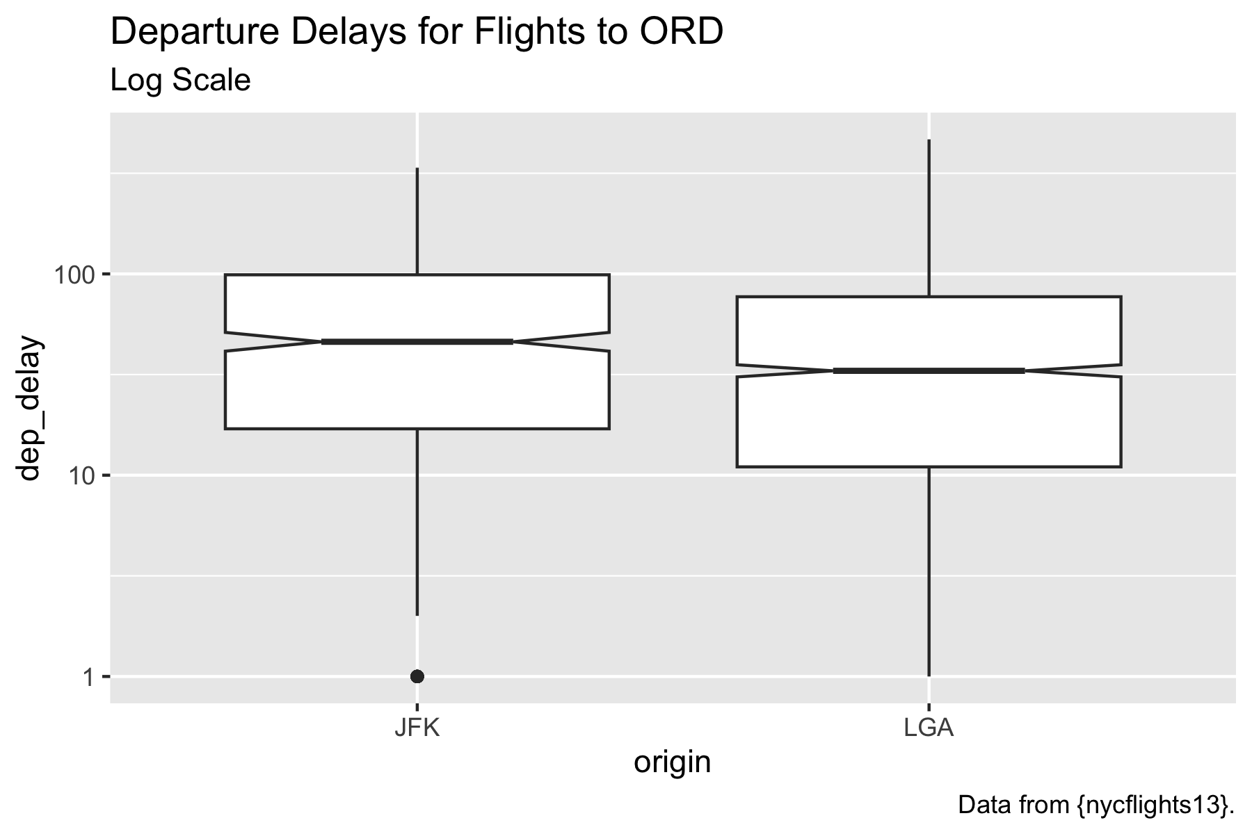
8.34.3 Using R Variables in SQL Code

You can also use an existing R variable as a value in a SQL query clause.

Create the R Variable and use the name preceded by a ?.

```{r}
my_dest <- 'MCO'
```

```{sql}
--| connection: con
--| output.var: "select_flights_df2"
SELECT
    DISTINCT "flight",
    "origin",
    "dest",
    "dep_delay"
FROM
    flights
WHERE
     ("origin" = 'JFK'
        OR "origin" = 'LGA')
    AND dest = ?my_dest;
```

glimpse(select_flights_df2)

Rows: 2,638
Columns: 4
$ flight    <int> 2159, 199, 1083, 1099, 2285, 83, 1815, 1443, 1685, 1815, 158…
$ origin    <chr> "JFK", "LGA", "JFK", "LGA", "LGA", "JFK", "JFK", "LGA", "LGA…
$ dest      <chr> "MCO", "MCO", "MCO", "MCO", "MCO", "MCO", "MCO", "MCO", "MCO…
$ dep_delay <dbl> -1, -5, 46, 0, 29, -1, -6, -3, -7, -7, 18, 1, -5, 0, -8, -4,…

Warning

Using parameters in SQL queries is common practice.

Use R to manipulate text to create queries as character strings is also common.

However, if you are building something, e.g., a Shiny app, where you are allowing others to input text that will feed into a query, you have to protect what you are doing.

You are liable to be victim of a SQL Injection Attack which can have bad consequences.

For R-specific approaches to mitigate the risk, see Run Queries Safely Posit (2023c) from the Posit Best Practices in working with Databases. Posit (2023b)

8.34.4 Setting the Connection Once in a Document

If you are going to use the same connection for all (or most chunks) in a document, you can set the connection as an option in a setup chunk.

Let’s close the current con.

DBI::dbDisconnect(con, shutdown = TRUE)

Now create a new connection.

```{r}
#| label: lst-setup
#| message: false
library(DBI)
library(duckdb)
con2 <- dbConnect(duckdb(dbdir = "./data/flights.duckdb", read_only = TRUE))
knitr::opts_chunk$set(connection = 'con2')
```

Now run a SQL code chunk without stating the connection.

```{sql}
--| label: lst-test-setup
--| eval: false
SHOW TABLES
```

8.34.5 Close the Connection.

To avoid a warning when rendering the document, close the connection at the end.

DBI::dbDisconnect(con2, shutdown = TRUE)

8.35 Using the {dbplyr} Package to Translate {dplyr} into SQL

The {dbplyr} package allows you to use {dplyr} code and it will translate it into SQL to interact (through an established connection) with a Back-end server.

• Consider R as a higher-level language you use to access code written in C.
• The {shiny} package can be considered as providing a higher-level language to generate HTML from {shiny} code.
• You can consider {dbplyr} as a higher-level package that generates SQL from {dplyr} code.

Important

{dbplyr} works for many flavors of SQL and can generate many SQL expressions.

However it cannot always do everything. For more details see the {dbplyr} vignette on Function Translation.

Even if you can’t use {dbplyr} in your situation, you can still use it to generate SQL code you can see and use. That makes it a good tool for learning SQL since you know {dplyr}.

Let’s load {dbplyr} and {tidyverse} along with {DBI} and {duckdb}.

library(tidyverse)
library(dbplyr)
library(DBI)
library(duckdb)

Create the connection to the database.

con <- dbConnect(duckdb(dbdir = "./data/flights.duckdb", read_only = TRUE))

Retrieve a table from a SQL database using dplyr::tbl().

• Note you have to specify the source of the data, here the database connection, and the table name.

flights2 <- tbl(src = con, "flights")

class(flights2)

[1] "tbl_duckdb_connection" "tbl_dbi"               "tbl_sql"              
[4] "tbl_lazy"              "tbl"                  

names(flights2)

[1] "src"        "lazy_query"

• Note that flights2 is not a data frame. It’s a list with class tbl_duckdb_connection.

Now you can use your tidyverse code on the flights table to generate a query.

flights2 |>
  select(flight, origin, dest, dep_delay) |>
  filter(origin == "JFK", dest == "CMH") |>
  summarize(dep_delay = mean(dep_delay, na.rm = TRUE)) ->
  my_query

my_query

# Source:   SQL [?? x 1]
# Database: DuckDB 1.4.4 [root@Darwin 25.3.0:R 4.5.2//Users/rressler/Courses/DATA-413-613/lectures_book/data/flights.duckdb]
  dep_delay
      <dbl>
1      22.0

class(my_query)

[1] "tbl_duckdb_connection" "tbl_dbi"               "tbl_sql"              
[4] "tbl_lazy"              "tbl"                  

Execute the query by using collect() at the end.

flights2 |>
  select(flight, origin, dest, dep_delay) |>
  filter(origin == "JFK", dest == "CMH") |>
  summarize(dep_delay = mean(dep_delay, na.rm = TRUE)) |>
  collect() ->
  my_result

my_result

# A tibble: 1 × 1
  dep_delay
      <dbl>
1      22.0

class(my_result)

[1] "tbl_df"     "tbl"        "data.frame"

To see the SQL code that was generated, use show_query() at the end (this is a good way to learn SQL).

flights2 |>
  select(flight, origin, dest, dep_delay) |>
  filter(origin == "JFK", dest == "CMH") |>
  summarize(dep_delay = mean(dep_delay, na.rm = TRUE)) |>
  show_query()

<SQL>
SELECT AVG(dep_delay) AS dep_delay
FROM (
  SELECT flight, origin, dest, dep_delay
  FROM flights
  WHERE (origin = 'JFK') AND (dest = 'CMH')
) q01

After you are done with the database, close the connection.

DBI::dbDisconnect(con, shutdown = TRUE)

8.36 The DBeaver Integrated Development Environment (IDE)

• This section based on work by Professor David Gerard.

There is a free, separate Front-end for the DuckDB database called “DBeaver Community”.

Per DBeaver community:

DBeaver Community is a free cross-platform database tool for developers, database administrators, analysts, and everyone working with data. It supports all popular SQL databases like MySQL, MariaDB, PostgreSQL, SQLite, Apache Family, and more.

8.36.1 Setup DBeaver Community

The instructions here are only for DuckDB. But DBeaver works with other DBMS’s pretty easily.

Download and install DBeaver Community here: https://dbeaver.io/download/.

When you open it up, select Database Navigator and under All or SQL, select “DuckDB”.

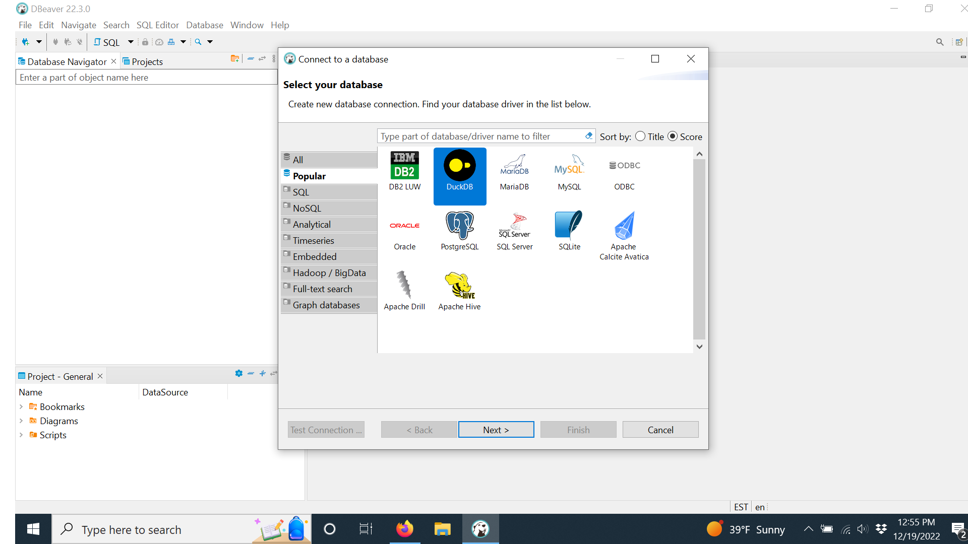
Then select Next.

Select “Host”, and Open to navigate to your flights.duckdb database.

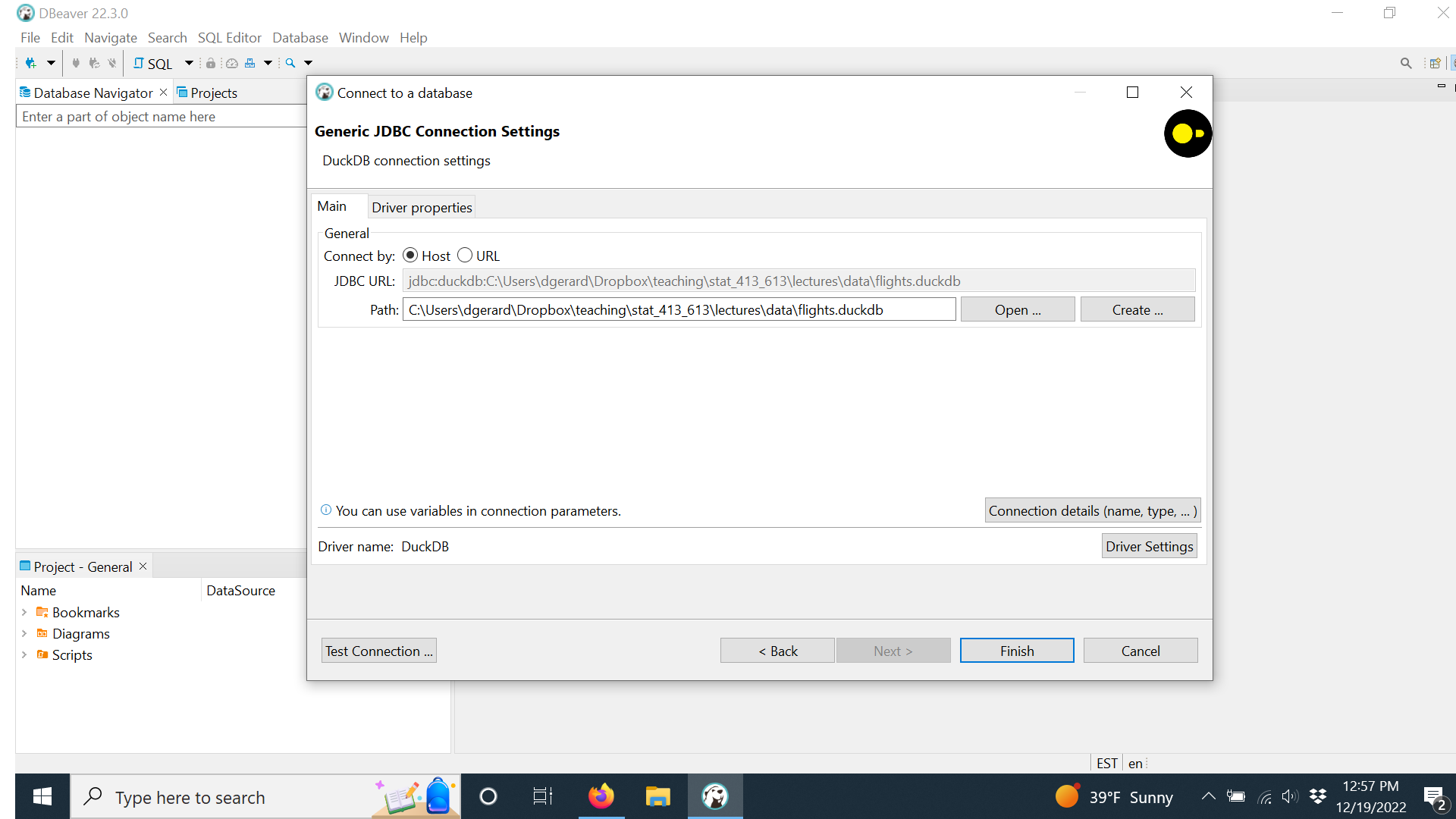
Click on Test Connection.

If Successful, you will get a pop-up window with the results of the test and which will allow you to see the details of the connection.

If not successful, and you haven’t used it before, it may ask you to install a JDBC-compliant driver to use to connect to a DuckDB database.

• Click Download Driver.
• After the download, it will run the test and you should get a positive result.

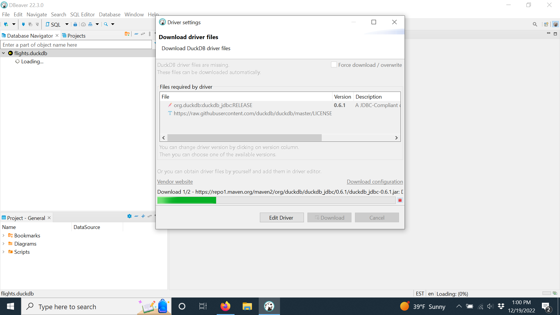
• Click “Finish”.

• You should now see the database under the Database Navigator.

• Right click on the connection and create a new SQL script file.

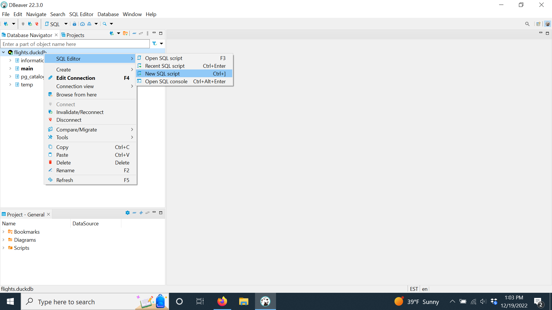
• Type some SQL and hit the execute button or just hit Control + Enter.

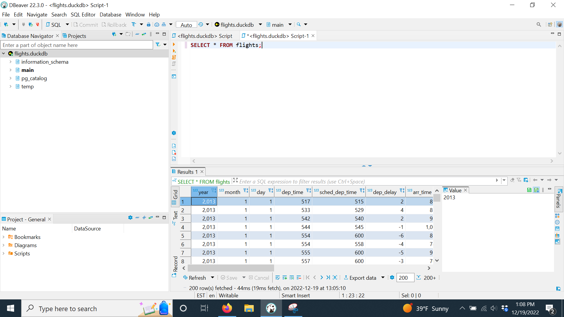
You can now play around with SQL.

When you want to save the data to a CSV file, just hit “Export data”.

There are a lot of features in DBeaver, but we won’t cover them. They are pretty intuitive. Just play with it for awhile.

• See the DBeaver General User Guide for detailed documentation.

8.36.2 Exercises

Use DBeaver for all of these exercises.

1. What is the mean temperature for flights from each airport?

SELECT "origin", AVG("temp") AS "temp"
FROM weather 
GROUP BY "origin";

2. What is the average number of flights from each airport per day in January?

SELECT "origin", COUNT() / 31.0 AS "ave"
FROM flights 
WHERE "month" = 1
GROUP BY "origin";

3. What are the top destinations for each airport?

SELECT "origin", "dest", "n"
FROM
(
SELECT "origin", "dest", "n", MAX("n") OVER (PARTITION BY "origin") AS "nmax"
FROM
(
SELECT "origin", "dest", COUNT() AS "n",
FROM flights
GROUP BY "origin", "dest"
)
)
WHERE "n" = "nmax"

8.37 Considerations for Working with SQL and Databases

8.37.1 Review Documentation about the database

When working with a new database, or one that is evolves over time, start by reviewing the available documentation.

Data dictionaries, schema descriptions, and E-R diagrams help you understand:

• Table structure and purpose
• Field definitions and data types
• Primary and foreign keys
• Indexes and constraints

This documentation gives you a holistic picture of the data so you can:

• Identify the correct tables and fields
• Understand the grain of each table
• Join tables correctly and efficiently

Many databases also follow naming conventions for tables and fields.

• Learning those conventions can dramatically reduce your search time.

8.37.2 Review Documentation about the DBMS and its SQL Dialect

Every DBMS implements its own “flavor” of SQL.

• Even though SQL is standardized, vendors optimize their systems differently and add extensions.

Review the documentation for:

• Supported syntax and functions
• Performance characteristics
• Indexing behavior
• Query planner behavior

Many dialects include features that simplify code or improve performance.

8.37.3 Choose a Front-End IDE That Supports Your Workflow

SQL is plain text, so it can be written anywhere. However, productivity improves significantly with the right tools.

If you are doing substantial SQL work, consider a SQL-focused IDE with features such as:

• Auto-complete
• Query formatting
• Execution plan visualization
• Schema browsing

For example, DBeaver provides SQL formatting and execution plan tools that RStudio does not.

Choose a front-end that works well with the DBMS in your organization and supports multiple connections if needed.

8.37.4 Follow a Style Guide

Readable SQL is easier to debug, review, and maintain. At minimum:

• Put major clauses on separate lines
• Align keywords vertically
• Indent logically
• Use consistent capitalization

Both of the following code chunks are valid SQL.

Streaming SQL example.

```{sql}
--| eval: false
--| connection: con
SELECT "flight", "origin", CASE WHEN ("origin" = 'JFK') THEN 'John F. Kennedy' WHEN ("origin" = 'LGA') THEN 'LaGaurdia' WHEN ("origin" = 'EWR') THEN 'Newark Liberty' ELSE 'WHO KNOWS' END AS "orig_long" FROM flights LIMIT 10;
```

Stylized tidy SQL.

```{sql}
--| label: tidy-sql
--| eval: false
--| connection: con
SELECT
    "flight",
    "origin",
    CASE
        WHEN "origin" = 'JFK' THEN 'John F. Kennedy'
        WHEN "origin" = 'LGA' THEN 'LaGuardia'
        WHEN "origin" = 'EWR' THEN 'Newark Liberty'
        ELSE 'WHO KNOWS'
    END AS "orig_long"
FROM flights
LIMIT 10;
```

Which do you think is easier to read, debug, and maintain?

• The second chunk was generated by the DBeaver Format SQL command under the Edit menu.

There is no single authoritative style guide so check if your organization has its own.

If it does not, consider the following.

• SQL Style Guide
• GitLab SQL Style Guide
• Basic SQL Debugging

Readable SQL reduces debugging time.

8.37.5 Build-a-little-test-a-little

Writing and debugging SQL queries should proceed in steps just like building and debugging R code and functions.

Don’t write a 30 line query and then start to debug it. Instead:

1. Start with a small SELECT
2. Add one clause at a time
3. Use LIMIT
4. Verify row counts after each join
5. Use EXPLAIN ANALYZE when behavior is surprising

Complex queries are easier to build incrementally using:

• Subqueries
• Common Table Expressions (CTEs)

8.37.6 Follow Best Practices for Query Design

Common performance and clarity principles include:

1. Return only the columns you need.
2. Avoid SELECT * in production queries.
3. Shape queries so indexes can be used efficiently.
4. Avoid leading wildcards in LIKE '%value' searches.
5. Prefer explicit joins over implicit comma joins. Use aliases (AS) for clarity.
6. Avoid unnecessary sorting on large tables.
7. Use comments -- to explain why you are doing something.

Modern databases rarely “lock” tables for simple reads, but poorly scoped queries still consume CPU, memory, and I/O resources.

For additional recommendations and rationale, consider the following as a starting point.

• 7 Bad Practices to Avoid When Writing SQL Queries for Better Performance Allam (2023) is a good place to start.
• Best Practices for Writing SQL Queries Metabase (2023) has an extensive list of suggestions.

8.37.7 Understand the Query Execution Lifecycle

Queries go through three stages when being executed.

• Syntax Check: The DBMS parser checks each query is syntactically correct.
• Optimization: The DBMS optimizer examines the query and builds a plan for execution to minimize resource demand and time.
• Execution: The DBMS runs the optimized plan to return any results.

Thus every query gets optimized but that does not mean the query could not be tuned to be faster.

If you have a query that is run many times, on large tables, and appears slow, then consider tuning it.

The first step is detecting a slow query.

• Most DBMS have a way to monitor query performance.
• For DBeaver, see 3 Ways to Detect Slow Queries in PostgreSQL. Schönig (2018)

The second step to is to assess how the query is actually being run.

• DBMS also have a way get to the results of the Query Planner so you can review them to see what is actually happening.
• Look at the help for EXPLAIN.
• For DBeaver, review the PostgreSQL Documentation on Using EXPLAIN Group (2023)

Once you understand the execution, then consider if any of the best practices for writing queries will help improve performance.

For more explanation and ideas see SQL Performance Tuning. khushboogoyal499 (2022)

8.37.8 Integrate Your SQL Into Your Version Control Workflow

SQL files are text and should be version controlled..

• Version control provides change tracking, facilitates collaboration, and enhances reproducibility

Store .sql files in Git repositories just like R or Python scripts.

• If you are using DBeaver, use the search tool (magnifying glass) and look for “Install new software.”
• Use the drop down arrow to select the Git option as in Figure 8.5.

Figure 8.5: Installing the DBeaver Extension for Git

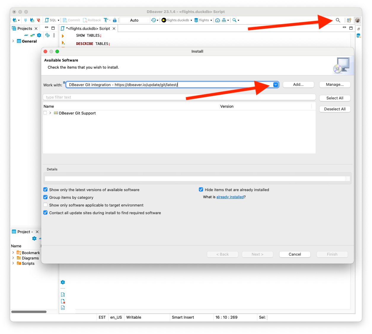
For more details see How to Version Control Your SQL.

8.37.9 Expand Your SQL Knowledge Over Time

These notes cover core concepts, but learning more about advanced features can help your effectiveness:

• Views
• Window functions
• Advanced joins
• CTEs and recursive queries
• Stored procedures
• Dynamic SQL

There are many free references on SQL to expand your knowledge.

R for Data Science suggests two non-free books:

• SQL for Data Scientists
• Practical SQL: A Beginner’s Guide to Storytelling with Data.

8.37.10 Strategize How to Use SQL in Your Analysis Workflow

From a data science perspective SQL is usually a means for getting data out of databases.

• Data scientists are usually less involved in designing, building, and managing databases or maintaining the data.

Your working environment will often dictate which databases have the data of interest and the associated versions of SQL you must use.

There are SQL wizards who can make SQL dance by building and optimizing queries to the n^th degree.

• You do not have to be one!
• As long as you can get the data you need, you can use the other tools in R and Python to make your analysis sing and dance.

Use SQL to Filter, Aggregate, Join, and Subset to get the data you need in a useful form.

SQL is an important tool in your Data Science tool box for sure. But it works best when you use it with other tools in it as well.

Tip

If your primary analysis tools are R and RStudio/Positron, but you need to get subsets of data from a large database using SQL, consider using a SQL-focused IDE, such as DBeaver, to build your queries and then copying them into a .sql file or an SQL code chunk.

This way you get the advantage of using a SQL-focused IDE while using RStudio/Positron for the rest of the analysis workflow.

8.38 SQL Interview Prep with DuckDB”

8.38.1 SQL Syntax Cheat Sheet (DuckDB)

Task	DuckDB Syntax
Limit rows	SELECT * FROM table LIMIT 5;
String concat	first_name || ' ' || last_name
Current date/time	NOW()
Date difference (days)	julianday(date1) - julianday(date2)
Pagination	LIMIT 10 OFFSET 20
Conditional logic	CASE WHEN score > 90 THEN 'A' ELSE 'B' END
Random row	ORDER BY RANDOM()
String search	WHERE name LIKE '%abc%'
Joins	JOIN ... ON ...
Aggregation	GROUP BY + HAVING

8.38.2 Concept Questions

1. Grain and Keys
   • What is the grain of a table?
   • How do you determine if a column (or combination) uniquely identifies rows?
   • What happens if you join at the wrong grain?
   • Difference between:
     • Natural key
     • Composite key
     • Surrogate key
   • How would you verify whether a column is truly unique in a production table?

1. Grain and Keys

-   What is the grain of a table?
  - The grain defines what one row represents — the level of detail at which the data is stored.
  
-   How do you determine if a column (or combination) uniquely identifies rows?
  - Verify that the number of rows equals the number of distinct values in that column (or combination).

-   What happens if you join at the wrong grain?
  - You create unintended row multiplication because multiple rows match per key, leading to incorrect aggregates and inflated results.

-   Difference between natural key, composite key, surrogate key?
    - A natural key has business meaning, a composite key uses multiple columns together for uniqueness, and a surrogate key is an artificial identifier with no business meaning.

-   How would you verify whether a column is truly unique in production?
    -Compare total row count to distinct count and investigate any duplicates before trusting it as a join key.

2. Join Cardinality and Row Explosion.
   • Explain the following:
     • One-to-one vs one-to-many vs many-to-many
     • How to detect unintended row multiplication
     • How to debug joins using COUNT(*)
     • How to use EXPLAIN ANALYZE
   • A join increased your row count by 10x. What are the first three things you check?

2. Join Cardinality and Row Explosion

- One-to-one vs one-to-many vs many-to-many?
    - One-to-one preserves row count, one-to-many increases rows on one side, and many-to-many can multiply rows dramatically.

- How to detect unintended row multiplication?
    - Compare row counts before and after the join and look for unexpected growth.

- How to debug joins using `COUNT(*)`?
    - Count rows from each table independently, then count the joined result to see if multiplication occurred.

- How to use `EXPLAIN ANALYZE`?
    - It shows the execution plan and actual row counts at each step, helping identify where row growth occurs.

- A join increased row count by 10x — first three checks?
    - Confirm the grain of both tables, verify the join keys are complete, and check whether the right table is unique on the join key.

3. NULL Logic
   • Explain
     • Why my_field = NULL doesn’t work
       • Three-valued logic
       • The NOT IN + NULL trap
       • The difference between COUNT(*) and COUNT(column)

• Why can NOT IN (subquery) unexpectedly return zero rows?

3. NULL Logic

- Why `my_field = NULL` doesn’t work?
  - Because `NULL` represents unknown, and comparisons to unknown evaluate to `UNKNOWN`, not `TRUE`.

- Three-valued logic?
    - SQL evaluates conditions as `TRUE`, `FALSE`, or `UNKNOWN`, and only `TRUE` rows are kept by `WHERE`.

-   The `NOT IN` + `NUL`L trap?
    - If a subquery contains even one `NULL`, the entire `NOT IN` comparison becomes `UNKNOWN` for all rows.

- Difference between `COUNT(*)` and `COUNT(column)`?
    - `COUNT(*)` counts all rows; `COUNT(column)` ignores `NULL` values.

- Why can NOT IN (subquery) return zero rows?
    - Because if the subquery includes `NULL`, every comparison becomes `UNKNOWN` and no rows qualify.

4. Execution Order of SQL
   • What is the logical execution order of a SELECT statement?

4. Execution Order of SQL

Logical execution order is: 

FROM -> WHERE -> GROUP BY -> HAVING -> SELECT -> ORDER BY -> LIMIT.

5. Window Functions
   • Difference between GROUP BY and window functions
     • When to use ROW_NUMBER() vs RANK()
     • How to compute percent of total using window functions

5. Window Functions

- Difference between `GROUP BY` and window functions?
    - `GROUP BY` collapses rows into summaries; window functions compute group-based values while preserving all original rows.

- When to use `ROW_NUMBER()` vs `RANK()`?
    - Use `ROW_NUMBER()` when ties must be broken uniquely;
    - Use `RANK()` when tied values should share the same rank.

- How to compute percent of total using window functions?
    - Divide the row value by a windowed SUM over the appropriate partition.

6. Explain the differences between the following:
   • WHERE vs HAVING
   • JOIN vs UNION
   • INNER JOIN vs LEFT JOIN
   • DISTINCT vs GROUP BY
   • CTE vs subquery
   • Window function vs GROUP BY

6. Concept Comparisons

- `WHERE` vs `HAVING`?
    - `WHERE` filters rows before aggregation; 
    - `HAVING` filters groups after aggregation.

-   `JOIN` vs `UNION`?
    - `JOIN` combines columns from tables side-by-side; 
    - `UNION` stacks rows vertically.

- `INNER JOIN` vs `LEFT JOIN`?
    - `INNER` returns only matching rows; 
    - `LEFT returns all left rows and `NULL` for unmatched right rows.

- `DISTINCT` vs `GROUP BY`?
    - `DISTINCT` removes duplicate rows; 
    - `GROUP BY` groups rows for aggregation.

- CTE vs subquery?
    - A CTE is a named temporary result used within a query; 
    - A subquery is an inline nested query.

- Window function vs `GROUP BY`?
    - Window functions add grouped calculations without collapsing rows; 
    - `GROUP BY` collapses rows into summary output.

8.38.3 Coding Questions

• Create Example Schema

library(DBI)
library(duckdb)
con <- dbConnect(duckdb::duckdb(), dbdir = ":memory:")

dbExecute(con, "
CREATE TABLE departments (
  department_id INTEGER PRIMARY KEY,
  department_name VARCHAR
);
")

[1] 0

dbExecute(con, "
CREATE TABLE employees (
  employee_id INTEGER PRIMARY KEY,
  name VARCHAR,
  department_id INTEGER,
  salary DOUBLE,
  hire_date DATE,
  manager_id INTEGER,
  birthdate DATE,
  FOREIGN KEY (department_id) REFERENCES departments(department_id)
);
")

[1] 0

dbExecute(con, "
INSERT INTO departments VALUES
(1, 'Engineering'),
(2, 'HR'),
(3, 'Finance'),
(4, 'Operations');
")

[1] 4

dbExecute(con, "
INSERT INTO employees VALUES
(1, 'Alice', 1, 90000, '2020-01-15', NULL, '1990-06-05'),
(2, 'Bob', 1, 80000, '2021-03-22', 1, '1985-09-12'),
(3, 'Charlie', 2, 70000, '2019-07-10', 1, '1992-01-25'),
(4, 'Diana', 3, 95000, '2022-02-18', 1, '1988-12-11'),
(5, 'Eve', 3, 87000, '2021-10-05', 4, '1995-04-17'),
(6, 'Frank', 4, 65000, '2020-06-30', 1, '1993-07-09'),
(7, 'Grace', 4, 64000, '2022-05-15', 6, '1991-08-19');
")

[1] 7

1. Top 3 Salaries

SELECT * FROM employees
ORDER BY salary DESC
LIMIT 3;

3 records

employee_id	name	department_id	salary	hire_date	manager_id	birthdate
4	Diana	3	95000	2022-02-18	1	1988-12-11
1	Alice	1	90000	2020-01-15	NA	1990-06-05
5	Eve	3	87000	2021-10-05	4	1995-04-17

1. Average Salary by Department

SELECT department_id, AVG(salary) AS avg_salary
FROM employees
GROUP BY department_id;

4 records

department_id	avg_salary
1	85000
2	70000
3	91000
4	64500

3. Rank Employees by Salary (Window Function)

SELECT name, salary,
       RANK() OVER (ORDER BY salary DESC) AS salary_rank
FROM employees;

7 records

name	salary	salary_rank
Diana	95000	1
Alice	90000	2
Eve	87000	3
Bob	80000	4
Charlie	70000	5
Frank	65000	6
Grace	64000	7

4. Salary vs Department Average (Window Function)

SELECT name, salary,
       AVG(salary) OVER (PARTITION BY department_id) AS dept_avg_salary,
       salary - AVG(salary) OVER (PARTITION BY department_id) AS salary_diff
FROM employees;

7 records

name	salary	dept_avg_salary	salary_diff
Alice	90000	85000	5000
Bob	80000	85000	-5000
Diana	95000	91000	4000
Eve	87000	91000	-4000
Frank	65000	64500	500
Grace	64000	64500	-500
Charlie	70000	70000	0

5. Employees Above Department Average (Subquery)

SELECT name, salary, department_id
FROM employees e
WHERE salary > (
    SELECT AVG(salary)
    FROM employees
    WHERE department_id = e.department_id
);

3 records

name	salary	department_id
Alice	90000	1
Diana	95000	3
Frank	65000	4

6. Managers and Their Direct Reports

SELECT m.name AS manager_name,
       e.name AS employee_name
FROM employees e
JOIN employees m
  ON e.manager_id = m.employee_id
ORDER BY manager_name;

6 records

manager_name	employee_name
Alice	Bob
Alice	Charlie
Alice	Diana
Alice	Frank
Diana	Eve
Frank	Grace

7. Department Headcount

SELECT d.department_name,
       COUNT(e.employee_id) AS headcount
FROM departments d
LEFT JOIN employees e
  ON d.department_id = e.department_id
GROUP BY d.department_name;

4 records

department_name	headcount
Finance	2
HR	1
Operations	2
Engineering	2

8. Youngest Employee in Each Department (Window Function)

SELECT name, department_id, birthdate
FROM (
  SELECT name, department_id, birthdate,
         ROW_NUMBER() OVER (PARTITION BY department_id ORDER BY birthdate DESC) AS rn
  FROM employees
) t
WHERE rn = 1;

4 records

name	department_id	birthdate
Eve	3	1995-04-17
Charlie	2	1992-01-25
Frank	4	1993-07-09
Alice	1	1990-06-05

9. Employees Hired in the Last 2 Years

SELECT name, hire_date
FROM employees
WHERE hire_date >= DATE '2023-01-01';

0 records

name	hire_date

10. Employees Who Are Not Managers - Hint - Consider NOT EXIST

SELECT e.employee_id, e.name
FROM employees e
WHERE NOT EXISTS (
  SELECT 1
  FROM employees r
  WHERE r.manager_id = e.employee_id
)
ORDER BY e.employee_id;

4 records

employee_id	name
2	Bob
3	Charlie
5	Eve
7	Grace

11. Close the connection.

dbDisconnect(conn = con, shutdown = TRUE)

Aden-Buie, Garrick. 2020. “Starwarsdb: Relational Data from the ’Star Wars’ API for Learning and Teaching.” https://cran.r-project.org/web/packages/starwarsdb/index.html.

Allaire, J. J. 2023. “RStudio: Code Snippets in the RStudio IDE.” Posit Support. https://support.posit.co/hc/en-us/articles/204463668-Code-Snippets-in-the-RStudio-IDE.

Allam, Abdelrahman Mohamed. 2023. “SQL: 7 Bad Practices to Avoid When Writing SQL Queries for Better Performance 🚀.” DEV Community. https://dev.to/abdelrahmanallam/7-bad-practices-to-avoid-when-writing-sql-queries-for-better-performance-c87.

Codd, E. F. 1970. “A Relational Model of Data for Large Shared Data Banks.” Communications of the ACM 13 (6): 377–87. https://doi.org/10.1145/362384.362685.

David-Engel. 2023. “ODBC: Microsoft Open Database Connectivity (ODBC) - Open Database Connectivity (ODBC).” https://learn.microsoft.com/en-us/sql/odbc/microsoft-open-database-connectivity-odbc?view=sql-server-ver16.

DuckDB. 2023a. “DBeaver SQL IDE.” DuckDB. https://duckdb.org/docs/guides/sql_editors/dbeaver.html.

———. 2023b. “DuckDB Installation.” DuckDB. https://duckdb.org/docs/installation/.

———. 2023c. “DuckDB: An in-Process SQL OLAP Database Management System.” DuckDB. https://duckdb.org/.

Explorer, Internet. 2023. “The Trade-offs Between Database Normalization and Denormalization.” DEV Community. https://dev.to/er_dward/the-trade-offs-between-database-normalization-and-denormalization-4kdo.

Foundation, MariaDB. 2023a. “Basic SQL Debugging.” MariaDB KnowledgeBase. https://mariadb.com/kb/en/basic-sql-debugging/.

———. 2023b. “Database Theory.” MariaDB KnowledgeBase. https://mariadb.com/kb/en/database-theory/.

Group, PostgreSQL Global Development. 2023. “SQL: PostgreSQL Using EXPLAIN.” PostgreSQL Documentation. https://www.postgresql.org/docs/15/using-explain.html.

Hester, Jim, Hadley Wickham, and Oliver Gjoneski. 2023. “Odbc: Connect to ODBC Compatible Databases (Using the DBI Interface).” https://r-dbi.github.io/odbc/.

Holywell, Simon. 2023. “SQL Style Guide by Simon Holywell.” https://www.sqlstyle.guide.

khushboogoyal499. 2022. “SQL Performance Tuning.” GeeksforGeeks. https://www.geeksforgeeks.org/sql-performance-tuning/.

kingthorin, and OWASP Foundation. 2023. “SQL Injection.” https://owasp.org/www-community/attacks/SQL_Injection.

mermaid.js. 2023. “Mermaid Diagramming and Charting Tool.” http://mermaid.js.org/.

Mestel, Craig, and Amie Bright. 2023. “SQL Style Guide - GitLab.” GitLab. https://about.gitlab.com/handbook/business-technology/data-team/platform/sql-style-guide/.

Metabase. 2023. “SQL: Best Practices for Writing SQL Queries.” Metabase Business Intelligence, Dashboards, and Data Visualization. https://www.metabase.com/learn/sql-questions/sql-best-practices.

Mühleisen, Hannes, Mark Raasveldt, Stichting DuckDB Foundation, Apache Software Foundation, PostgreSQL Global Development Group, The Regents of the University of California, Cameron Desrochers, et al. 2023. “Duckdb: DBI Package for the DuckDB Database Management System.” https://cran.r-project.org/web/packages/duckdb/index.html.

Posit. 2023a. “Dbplyr: Writing SQL with Dbplyr.” https://dbplyr.tidyverse.org/articles/sql.html.

———. 2023b. “Posit Solutions - Best Practices in Working with Databases.” https://solutions.posit.co/connections/db/.

———. 2023c. “Posit Solutions - Run Queries Safely.” https://solutions.posit.co/connections/db/best-practices/run-queries-safely/.

Pullum (Swartz), Erika. 2020. “SQL: How to Version Control Your SQL.” Substack Newsletter. Better with Data. https://betterwithdata.substack.com/p/how-to-version-control-your-sql.

R Special Interest Group on Databases (R-SIG-DB), Hadley Wickham, and Kirill Muller. 2022. “DBI: R Database Interface.” https://dbi.r-dbi.org/.

Schönig, Hans-Jürgen. 2018. “3 Ways to Detect Slow Queries in PostgreSQL.” CYBERTEC. https://www.cybertec-postgresql.com/en/3-ways-to-detect-slow-queries-in-postgresql/.

Schools, W3. 2023. “SQL Tutorial.” https://www.w3schools.com/sql/.

Team, DBeaver. 2003. “DBeaver User Guide.” GitHub. https://github.com/dbeaver/dbeaver/wiki/Home.

Ushey, Kevin. 2023. “RStudio: Customizing Keyboard Shortcuts in the RStudio IDE.” Posit Support. https://support.posit.co/hc/en-us/articles/206382178-Customizing-Keyboard-Shortcuts-in-the-RStudio-IDE.

w3resource. 2023. “SQL: Physicians Who Is the Head of Each Department.” W3resource. https://www.w3resource.com/sql-exercises/hospital-database-exercise/sql-exercise-hospital-database-3.php.

Wickham, Hadley, Mine Cetinkaya-Rundel, and Garrett Grolemund. 2023. R for Data Science (2e). O’Reilly Media, Inc. https://r4ds.hadley.nz/.

Wickham, Hadley, Maximilian Girlich, and Edgar Ruiz. 2023. “Dbplyr: A Dplyr Backend for Databases.” https://dbplyr.tidyverse.org/.

Xie, Yihui, J. J. Alllaire, and Garrett Grolemund. 2023. R Markdown: The Definitive Guide. https://bookdown.org/yihui/rmarkdown/.