16 Text Analysis 2

Published

March 31, 2026

Keywords

text analysis, tidytext, tf-idf, topic modeling, ngrams, dtm, corpus, quanteda

16.1 Introduction

16.1.1 Learning Outcomes

Expand strategies for analyzing text.
Manipulate and analyze text data from a variety of sources using the {tidytext} package for …
- Topic Modeling with TF-IDF Analysis.
- Analysis of ngrams.
- Converting to and from tidytext formats.

16.1.2 References:

{ggraph} package Pedersen (2022)
{igraph} package Csardi et al. (2023)
{janeaustenr} package Silge (2023)
{quanteda} package Benoit et al. (2018)
{sentimentr} package Rinker (2018)
Text Mining with R by Julia Silge and David Robinson Silge and Robinson (2025)
{tidytext} package Silge and Robinson (2016)
{tm} Text Mining Infrastructure package Feinerer and Hornik (2023)
{topicmodels} package Grün and Hornik (2023)

16.1.2.1 Other References

{matrix} package Bates, Maechler, and Jagan (2023)
{tidytext} website Silge and Robinson (2023a)
{tidytext} GitHub Silge and Robinson (2023b)
{widyr} package Robinson and Silge (2022)
{text2vec} package Selivanov (2023)
{word2vec} package “Word2vec Package” (2023)

16.2 Identifying Important Terms in a Corpus

We have done frequency analysis to study word usage and sentiment analysis to study emotional tone.

We now turn to methods for identifying terms and phrases that are important to one document relative to other documents in a corpus.

These methods can help us ask questions such as:

What words or phrases are most characteristic of a text?
How is one text similar to or different from other texts in the collection?
What terms help distinguish one document from another?

One way to compare a document with other documents is to examine the relative rates of word usage across them.

The other documents may be from a curated corpus, a general collection or group, or just a set of potentially similar works.

16.2.1 Term Frequency - Inverse Document Frequency (tf-idf)

Term Frequency is just how often a word (or term of multiple words) appears in a document (as we did before).

Higher is more important - as long as it is meaningful, i.e., not a stop word.

Inverse Document Frequency is a function that scores the frequency of word usage across multiple documents.

A word’s score (importance) decreases if it is used across multiple documents - it’s more common.
A word’s score (importance) increases if it is not used across multiple documents - it’s more specific to a document.

We multiply \(tf\) by \(idf\) to calculate the \(tf-idf\) for a term in a single document as part of a collection of documents, as shown in Table 16.1.

Table 16.1: Elements in \(tf-idf\)

Term Frequency (for a term in one document)	\(tf\)	\(\frac{n_{\text{term}}}{n_{\text{total words in the document}}}\)
Inverse Document Frequency (for a term across documents):	\(idf\)	\(\text{ln}\left(\frac{n_{\text{documents}}}{n_{\text{documents containing term}}}\right)\)
\(tf-idf\) (for a term in one document within a collection of documents)	\(tf-idf\)	\(tf \times idf\)

Important

The \(tf-idf\) is a heuristic measure of the relative importance of a term to a single document out of a collection of documents

These are the base formulas and they (or some extensions) are used in multiple NLP processes.
In practice, tf can be defined in slightly different ways. Here we use relative term frequency within each document.

16.2.1.1 TF in Jane Austen’s Novels

Load the {tidyverse}, {tidytext}, and {janeaustenr} packages.

library(tidyverse)
library(tidytext)
library(janeaustenr)

Count the total words and most commonly used words across the books.

Do not eliminate the stop words!
We want all the words to get the correct relative frequencies.

austen_books() |>
  unnest_tokens(word, text) |>
  mutate(word = str_extract(word, "[a-z']+")) |>
  count(book, word, sort = TRUE) ->
book_words

book_words |>
  group_by(book) |>
  summarize(total = sum(n), .groups = "drop") ->
total_words

book_words |>
  left_join(total_words, by = "book") ->
book_words

book_words

# A tibble: 39,708 × 4
   book              word      n  total
   <fct>             <chr> <int>  <int>
 1 Mansfield Park    the    6209 160460
 2 Mansfield Park    to     5477 160460
 3 Mansfield Park    and    5439 160460
 4 Emma              to     5242 160996
 5 Emma              the    5204 160996
 6 Emma              and    4897 160996
 7 Mansfield Park    of     4778 160460
 8 Pride & Prejudice the    4331 122204
 9 Emma              of     4293 160996
10 Pride & Prejudice to     4163 122204
# ℹ 39,698 more rows

Plot the tf for each book (should look familiar).

book_words |>
  ggplot(aes(n / total, fill = book)) +
  geom_histogram(show.legend = FALSE) +
  xlim(NA, 0.0009) +
  facet_wrap(~book, ncol = 2, scales = "free_y") +
  scale_fill_viridis_d(end = .8)

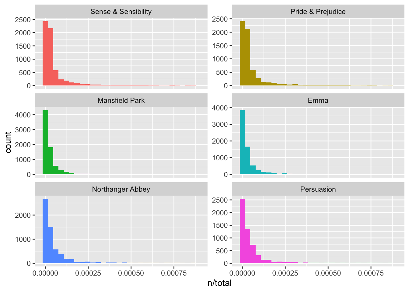
There are numerous words that only occur once in each book.

book_words |>
  filter(n == 1) |>
  nrow()

[1] 15929

Before moving to \(tf-idf\), it is useful to examine a broader pattern in word frequencies known as Zipf’s law.

16.2.1.2 Background on Zipf’s Law

The long-tailed distributions we just saw are common in language and are well-studied.

Zipf’s law, named after George Zipf, a 20^th century American linguist states:

The frequency of word is inversely proportional to its rank.
- Frequency is how often a word is used, and,
- Rank is the position of the word from the top of a list of the words sorted in descending order by their frequencies.
Example: the most frequently used word (rank = 1) might have frequency .05% and the rank 5 word might have frequency=.01% and so on.
Note, we are NOT removing stop words in these analyses as that would affect the distributions.

16.2.1.3 Zipf’s law for Jane Austen

Let’s look at how this applies in Jane Austen’s works.

book_words |>
  group_by(book) |>
  mutate(
    rank = row_number(),
    term_frequency = n / total
  ) ->
freq_by_rank

head(freq_by_rank, 10)

# A tibble: 10 × 6
# Groups:   book [3]
   book              word      n  total  rank term_frequency
   <fct>             <chr> <int>  <int> <int>          <dbl>
 1 Mansfield Park    the    6209 160460     1         0.0387
 2 Mansfield Park    to     5477 160460     2         0.0341
 3 Mansfield Park    and    5439 160460     3         0.0339
 4 Emma              to     5242 160996     1         0.0326
 5 Emma              the    5204 160996     2         0.0323
 6 Emma              and    4897 160996     3         0.0304
 7 Mansfield Park    of     4778 160460     4         0.0298
 8 Pride & Prejudice the    4331 122204     1         0.0354
 9 Emma              of     4293 160996     4         0.0267
10 Pride & Prejudice to     4163 122204     2         0.0341

Zipf’s law is often visualized by plotting rank on the x-axis and term frequency on the y-axis, on logarithmic scales.

Plotting this way, an inversely proportional relationship will have a constant, negative slope.

freq_by_rank |>
  ggplot(aes(rank, term_frequency, color = book)) +
  geom_line(size = 1.1, alpha = 0.8, show.legend = FALSE) +
  scale_x_log10() +
  scale_y_log10() +
  scale_color_viridis_d(end = .9)

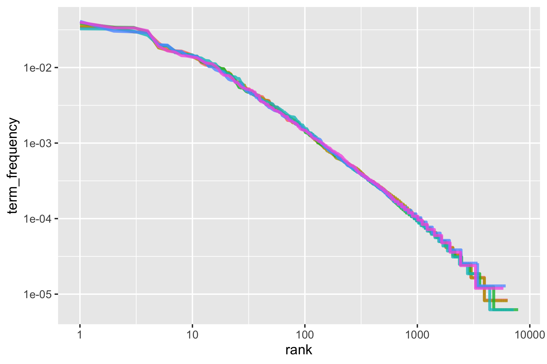
We can see the pattern is quite similar for all six novels - a negative slope.

It’s not quite linear though.

Let’s try to model the middle segment, between ranks 10 and 500, as linear.

freq_by_rank |>
  filter(rank < 500, rank > 10) ->
rank_subset

lmout <- lm(log10(term_frequency) ~ log10(rank), data = rank_subset)
broom::tidy(lmout)[c(1, 2, 5)]

# A tibble: 2 × 3
  term        estimate p.value
  <chr>          <dbl>   <dbl>
1 (Intercept)   -0.621       0
2 log10(rank)   -1.11        0

Classic versions of Zipf’s law have \(\text{frequency} \propto \frac{1}{\text{rank}}\).

Our model has a slope close to -1.
Let’s plot this fitted line.

coefs <- coef(lmout)
freq_by_rank |>
  ggplot(aes(rank, term_frequency, color = book)) +
  geom_abline(
    intercept = coefs[1], slope = coefs[2],
    color = "red", linetype = 2
  ) +
  geom_line(size = 1.1, alpha = 0.8, show.legend = FALSE) +
  scale_x_log10() +
  scale_y_log10() +
  scale_color_viridis_d(end = .9)

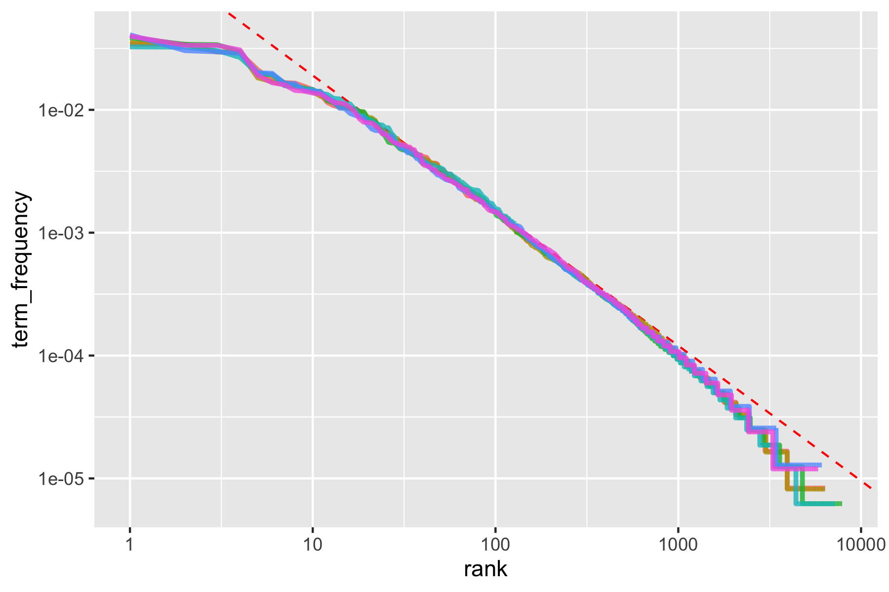
The result is close to the classic version of Zipf’s law for the corpus of Jane Austen’s novels.
- The deviations at high rank (> 1000) are not uncommon for many kinds of language; a corpus of language often contains fewer rare words than predicted by a single power law.
- The deviations at low rank (<10) are more unusual. Jane Austen uses a lower percentage of the most common words than many collections of language.

This kind of analysis could be extended to compare authors, or to compare any other collections of text; it can be implemented simply using tidy data principles.

There is a whole field to determining authorship through analysis of an author’s style called Stylometry. See Introduction to stylometry with Python for a nice introduction in Python.

16.2.2 Applying \(tf-idf\) to a Corpus

The bind_tf_idf() function calculates the tf-idf for us.

The idea of \(tf-idf\) is to identify words that are important to a specific document by

decreasing the weight (value) for words commonly used in a collection of other documents, and,
increasing the weight for words that are used less often across the other documents in the collection, (e.g., Jane Austen’s novels).

Calculating tf-idf attempts to find the words that are important (i.e., common) in a document, but not too common across documents.

Let’s use bind_tf_idf() on a tidytext-formatted tibble (one row per term (token), per document).

It returns a tibble with new columns tf, idf, and tf-idf.

book_words |>
  bind_tf_idf(word, book, n) ->
book_words

arrange(book_words, tf_idf, word) |> head(10)

# A tibble: 10 × 7
   book                word          n  total        tf   idf tf_idf
   <fct>               <chr>     <int>  <int>     <dbl> <dbl>  <dbl>
 1 Emma                a          3130 160996 0.0194        0      0
 2 Mansfield Park      a          3100 160460 0.0193        0      0
 3 Sense & Sensibility a          2092 119957 0.0174        0      0
 4 Pride & Prejudice   a          1954 122204 0.0160        0      0
 5 Persuasion          a          1594  83658 0.0191        0      0
 6 Northanger Abbey    a          1540  77780 0.0198        0      0
 7 Sense & Sensibility abilities     9 119957 0.0000750     0      0
 8 Pride & Prejudice   abilities     6 122204 0.0000491     0      0
 9 Mansfield Park      abilities     5 160460 0.0000312     0      0
10 Emma                abilities     3 160996 0.0000186     0      0

The \(idf\), and thus \(tf-idf\), are zero for extremely common words.

If they appear in all six novels, the \(idf\) term is \(log(1) = 0\).

In general, the \(idf\) (and thus \(tf-idf\)) is very low (near zero) for words that occur in many of the documents in a collection; this is how this approach decreases the weight for common words.

The \(idf\) will be higher for words that occur in fewer documents.

Let’s look at terms with high \(tf-idf\) in Jane Austen’s works.

book_words |>
  select(-total) |>
  arrange(desc(tf_idf)) |>
  head(10)

# A tibble: 10 × 6
   book                word          n      tf   idf  tf_idf
   <fct>               <chr>     <int>   <dbl> <dbl>   <dbl>
 1 Sense & Sensibility elinor      623 0.00519  1.79 0.00931
 2 Sense & Sensibility marianne    492 0.00410  1.79 0.00735
 3 Mansfield Park      crawford    493 0.00307  1.79 0.00551
 4 Pride & Prejudice   darcy       374 0.00306  1.79 0.00548
 5 Persuasion          elliot      254 0.00304  1.79 0.00544
 6 Emma                emma        786 0.00488  1.10 0.00536
 7 Northanger Abbey    tilney      196 0.00252  1.79 0.00452
 8 Emma                weston      389 0.00242  1.79 0.00433
 9 Pride & Prejudice   bennet      294 0.00241  1.79 0.00431
10 Persuasion          wentworth   191 0.00228  1.79 0.00409

As we saw before, the names of people and places tend to be important in each novel.

None of these occur in all of the novels and are primarily in one or two of them.

We can plot these.

book_words |>
  arrange(desc(tf_idf)) |>
  mutate(word = fct_rev(parse_factor(word))) |> ## ordering for ggplot
  group_by(book) |>
  slice_max(order_by = tf_idf, n = 10) |>
  ungroup() |>
  ggplot(aes(word, tf_idf, fill = book)) +
  geom_col(show.legend = FALSE) +
  labs(x = NULL, y = "tf-idf") +
  facet_wrap(~book, ncol = 2, scales = "free") +
  coord_flip() +
  scale_fill_viridis_d(end = .9)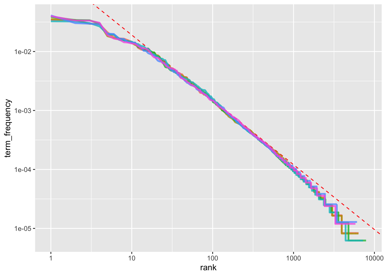

In this corpus, \(tf-idf\) highlights many proper nouns, suggesting that names of people and places are among the most distinctive terms for separating the novels.

This is the point of \(tf-idf\); it identifies words important to one document within a collection of documents.

16.2.2.1 Example: Using tf-idf to Analyze a Corpus of Physics Texts

Let’s download the following (translated) documents dealing with different ideas in science:

Discourse on Floating Bodies by Galileo Galilei, born 1564,
Treatise on Light by Christiaan Huygens, born 1629,
Experiments with Alternate Currents of High Potential and High Frequency by Nikola Tesla born 1856, and
Relativity: The Special and General Theory by Albert Einstein, born 1879.
The gutenberg ids are: 37729, 14725, 13476, and 30155.

Let’s include the authors as part of the meta-data we can select when we download them so we can download all at once.

Before we can use bind_tf_idf(), we have to unnest the terms, get rid of the formatting, and get the counts as before.

library(gutenbergr)
physics <- gutenberg_download(c(37729, 14725, 13476, 30155),
  meta_fields = "author"
)
physics |>
  unnest_tokens(word, text) |>
  mutate(word = str_extract(word, "[a-z']+")) |>
  count(author, word, sort = TRUE) ->
physics_words

physics_words |>
  head(10)

# A tibble: 10 × 3
   author              word      n
   <chr>               <chr> <int>
 1 Galilei, Galileo    the    3770
 2 Tesla, Nikola       the    3606
 3 Huygens, Christiaan the    3553
 4 Einstein, Albert    the    2995
 5 Galilei, Galileo    of     2051
 6 Einstein, Albert    of     2029
 7 Tesla, Nikola       of     1737
 8 Huygens, Christiaan of     1708
 9 Huygens, Christiaan to     1207
10 Tesla, Nikola       a      1176

We can now use bind_tf_idf() (which helps normalize across the documents of different lengths).

physics_words |>
  bind_tf_idf(word, author, n) |>
  mutate(word = fct_reorder(word, tf_idf)) |>
  mutate(author = factor(author, levels = c(
    "Galilei, Galileo",
    "Huygens, Christiaan",
    "Tesla, Nikola",
    "Einstein, Albert"
  ))) ->
physics_plot

Let’s plot the words by \(tf-idf\).

physics_plot |>
  group_by(author) |>
  slice_max(order_by = tf_idf, n = 15) |>
  ungroup() |>
  mutate(word = fct_reorder(word, tf_idf)) |>
  ggplot(aes(word, tf_idf, fill = author)) +
  geom_col(show.legend = FALSE) +
  labs(x = NULL, y = "tf-idf") +
  facet_wrap(~author, ncol = 2, scales = "free") +
  coord_flip() +
  scale_fill_viridis_d(end = .9)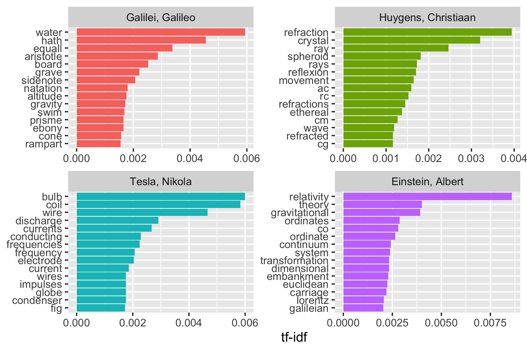

Note we have some unusual words due to how tidytext separates words by hyphens

We could get rid of them early in the process
We also have what appear to be abbreviations: RC, AC, CM, fig, cg, …

physics |>
  filter(str_detect(text, "RC")) |>
  select(text)

# A tibble: 44 × 1
   text                                                                  
   <chr>                                                                 
 1 line RC, parallel and equal to AB, to be a portion of a wave of light,
 2 represents the partial wave coming from the point A, after the wave RC
 3 be the propagation of the wave RC which fell on AB, and would be the  
 4 transparent body; seeing that the wave RC, having come to the aperture
 5 incident rays. Let there be such a ray RC falling upon the surface    
 6 CK. Make CO perpendicular to RC, and across the angle KCO adjust OK,  
 7 the required refraction of the ray RC. The demonstration of this is,  
 8 explaining ordinary refraction. For the refraction of the ray RC is   
 9 29. Now as we have found CI the refraction of the ray RC, similarly   
10 the ray _r_C is inclined equally with RC, the line C_d_ will          
# ℹ 34 more rows

We can remove these by creating our own custom stop words tibble and doing an anti-join.

mystopwords <- tibble(word = c(
  "eq", "co", "rc", "ac", "ak", "bn",
  "fig", "file", "cg", "cb", "cm",
  "ab"
))

physics_words <- anti_join(physics_words, mystopwords,
  by = "word"
)

plot_physics <- physics_words |>
  bind_tf_idf(word, author, n) |>
  mutate(word = str_remove_all(word, "_")) |>
  group_by(author) |>
  slice_max(order_by = tf_idf, n = 15) |>
  ungroup() |>
  mutate(word = reorder_within(word, tf_idf, author)) |>
  mutate(author = factor(author, levels = c(
    "Galilei, Galileo",
    "Huygens, Christiaan",
    "Tesla, Nikola",
    "Einstein, Albert"
  )))

ggplot(plot_physics, aes(word, tf_idf, fill = author)) +
  geom_col(show.legend = FALSE) +
  labs(x = NULL, y = "tf-idf") +
  facet_wrap(~author, ncol = 2, scales = "free") +
  coord_flip() +
  scale_x_reordered()+
  scale_fill_viridis_d(end = .9)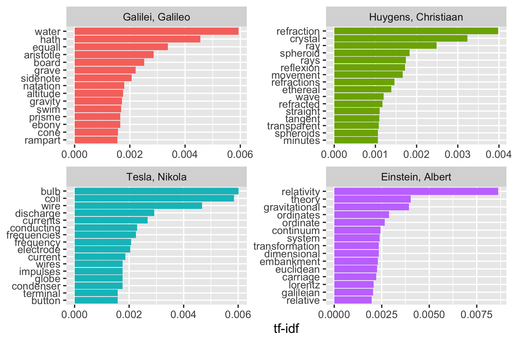

You could do more cleaning using regex and repeat the analysis.

Even at this level, it’s pretty clear the four books have something to do with water, light, electricity and gravity (yes, we could also read the titles).

16.2.3 TF-IDF Summary

The tf-idf approach allows us to find words that are characteristic of one document within a corpus or collection of documents, whether that document is a novel, a physics text, or a webpage.

16.3 Relationships Between Words: Analyzing n-Grams

We’ve analyzed words as individual units (within blocks of text of various sizes), and considered their relationships to sentiments or to documents.

We will now look at text analyses based on the relationships between groups of words, examining which words tend to follow others immediately, or, that tend to co-occur within the same documents.

16.3.1 Tokenizing by n-gram

We can use the function unnest_tokens() to create consecutive sequences of words, called n-grams.

By seeing how often word X is followed by word Y, we can build a model of the relationship between the two words.
We add the argument token = "ngrams" to unnest_tokens(), with the argument n = the number of words we wish to capture in each n-gram.
- n = 2 creates pairs of two consecutive words, often called a “bigram”.

Austen Books example.

austen_books() |>
  unnest_tokens(bigram, text, token = "ngrams", n = 2) ->
austen_bigrams
austen_bigrams

# A tibble: 675,025 × 2
   book                bigram         
   <fct>               <chr>          
 1 Sense & Sensibility sense and      
 2 Sense & Sensibility and sensibility
 3 Sense & Sensibility <NA>           
 4 Sense & Sensibility by jane        
 5 Sense & Sensibility jane austen    
 6 Sense & Sensibility <NA>           
 7 Sense & Sensibility <NA>           
 8 Sense & Sensibility <NA>           
 9 Sense & Sensibility <NA>           
10 Sense & Sensibility <NA>           
# ℹ 675,015 more rows

These bigrams overlap: “sense and” is one token, while “and sensibility” is another.

16.3.2 Counting and filtering n-Grams

Our usual tidy tools apply equally well to n-gram analysis.

austen_bigrams |>
  count(bigram, sort = TRUE)

# A tibble: 193,210 × 2
   bigram      n
   <chr>   <int>
 1 <NA>    12242
 2 of the   2853
 3 to be    2670
 4 in the   2221
 5 it was   1691
 6 i am     1485
 7 she had  1405
 8 of her   1363
 9 to the   1315
10 she was  1309
# ℹ 193,200 more rows

As you might expect, a lot of the most common bigrams are pairs of common (uninteresting) words.

We can get rid of these by using separate_wider_delim() and then removing rows where either word is a stop word.

austen_bigrams |>
  separate_wider_delim(bigram, names = c("word1", "word2"), delim = " ") ->
bigrams_separated

bigrams_separated |>
  filter(!word1 %in% stop_words$word) |>
  filter(!word2 %in% stop_words$word) ->
bigrams_filtered

## new bigram counts:
bigrams_filtered |>
  count(word1, word2, sort = TRUE) ->
bigram_counts

bigram_counts

# A tibble: 28,975 × 3
   word1   word2         n
   <chr>   <chr>     <int>
 1 <NA>    <NA>      12242
 2 sir     thomas      266
 3 miss    crawford    196
 4 captain wentworth   143
 5 miss    woodhouse   143
 6 frank   churchill   114
 7 lady    russell     110
 8 sir     walter      108
 9 lady    bertram     101
10 miss    fairfax      98
# ℹ 28,965 more rows

We can now unite() them back together.

bigrams_filtered |>
  unite(bigram, word1, word2, sep = " ") ->
bigrams_united

bigrams_united |>
  count(bigram, sort = TRUE)

# A tibble: 28,975 × 2
   bigram                n
   <chr>             <int>
 1 NA NA             12242
 2 sir thomas          266
 3 miss crawford       196
 4 captain wentworth   143
 5 miss woodhouse      143
 6 frank churchill     114
 7 lady russell        110
 8 sir walter          108
 9 lady bertram        101
10 miss fairfax         98
# ℹ 28,965 more rows

16.3.3 Analyzing bigrams

This one-bigram-per-row format is helpful for exploratory analyses of the text.

As a simple example, what are the most common “streets” mentioned in each book?

bigrams_filtered |>
  filter(word2 == "street") |>
  count(book, word1, sort = TRUE)

# A tibble: 33 × 3
   book                word1           n
   <fct>               <chr>       <int>
 1 Sense & Sensibility harley         16
 2 Sense & Sensibility berkeley       15
 3 Northanger Abbey    milsom         10
 4 Northanger Abbey    pulteney       10
 5 Mansfield Park      wimpole         9
 6 Pride & Prejudice   gracechurch     8
 7 Persuasion          milsom          5
 8 Sense & Sensibility bond            4
 9 Sense & Sensibility conduit         4
10 Persuasion          rivers          4
# ℹ 23 more rows

# or
bigrams_united |>
  filter(str_detect(bigram, "street")) |>
  count(book, bigram, sort = TRUE)

# A tibble: 51 × 3
   book                bigram                 n
   <fct>               <chr>              <int>
 1 Sense & Sensibility harley street         16
 2 Sense & Sensibility berkeley street       15
 3 Northanger Abbey    milsom street         10
 4 Northanger Abbey    pulteney street       10
 5 Mansfield Park      wimpole street         9
 6 Pride & Prejudice   gracechurch street     8
 7 Persuasion          milsom street          5
 8 Sense & Sensibility bond street            4
 9 Sense & Sensibility conduit street         4
10 Persuasion          rivers street          4
# ℹ 41 more rows

A bigram can also be treated as a “term” in a document in the same way we treated individual words.

We can calculate the \(tf-idf\) of bigrams.

bigrams_united |>
  count(book, bigram) |>
  bind_tf_idf(bigram, book, n) |>
  arrange(desc(tf_idf)) ->
bigram_tf_idf

bigram_tf_idf

# A tibble: 31,397 × 6
   book                bigram                n     tf   idf tf_idf
   <fct>               <chr>             <int>  <dbl> <dbl>  <dbl>
 1 Mansfield Park      sir thomas          266 0.0244  1.79 0.0438
 2 Persuasion          captain wentworth   143 0.0232  1.79 0.0416
 3 Mansfield Park      miss crawford       196 0.0180  1.79 0.0322
 4 Persuasion          lady russell        110 0.0179  1.79 0.0320
 5 Persuasion          sir walter          108 0.0175  1.79 0.0314
 6 Emma                miss woodhouse      143 0.0129  1.79 0.0231
 7 Northanger Abbey    miss tilney          74 0.0128  1.79 0.0229
 8 Sense & Sensibility colonel brandon      96 0.0115  1.79 0.0205
 9 Sense & Sensibility sir john             94 0.0112  1.79 0.0201
10 Emma                frank churchill     114 0.0103  1.79 0.0184
# ℹ 31,387 more rows

And plot as well.

bigram_tf_idf |>
  group_by(book) |>
  slice_max(order_by = tf_idf, n = 10) |>
  ungroup() |>
  mutate(bigram = reorder_within(bigram, tf_idf, book)) |>
  ggplot(aes(bigram, tf_idf, fill = book)) +
  geom_col(show.legend = FALSE) +
  labs(x = NULL, y = "tf-idf") +
  facet_wrap(~book, ncol = 2, scales = "free") +
  coord_flip() +
  scale_x_reordered() +
  scale_fill_viridis_d(end = .9)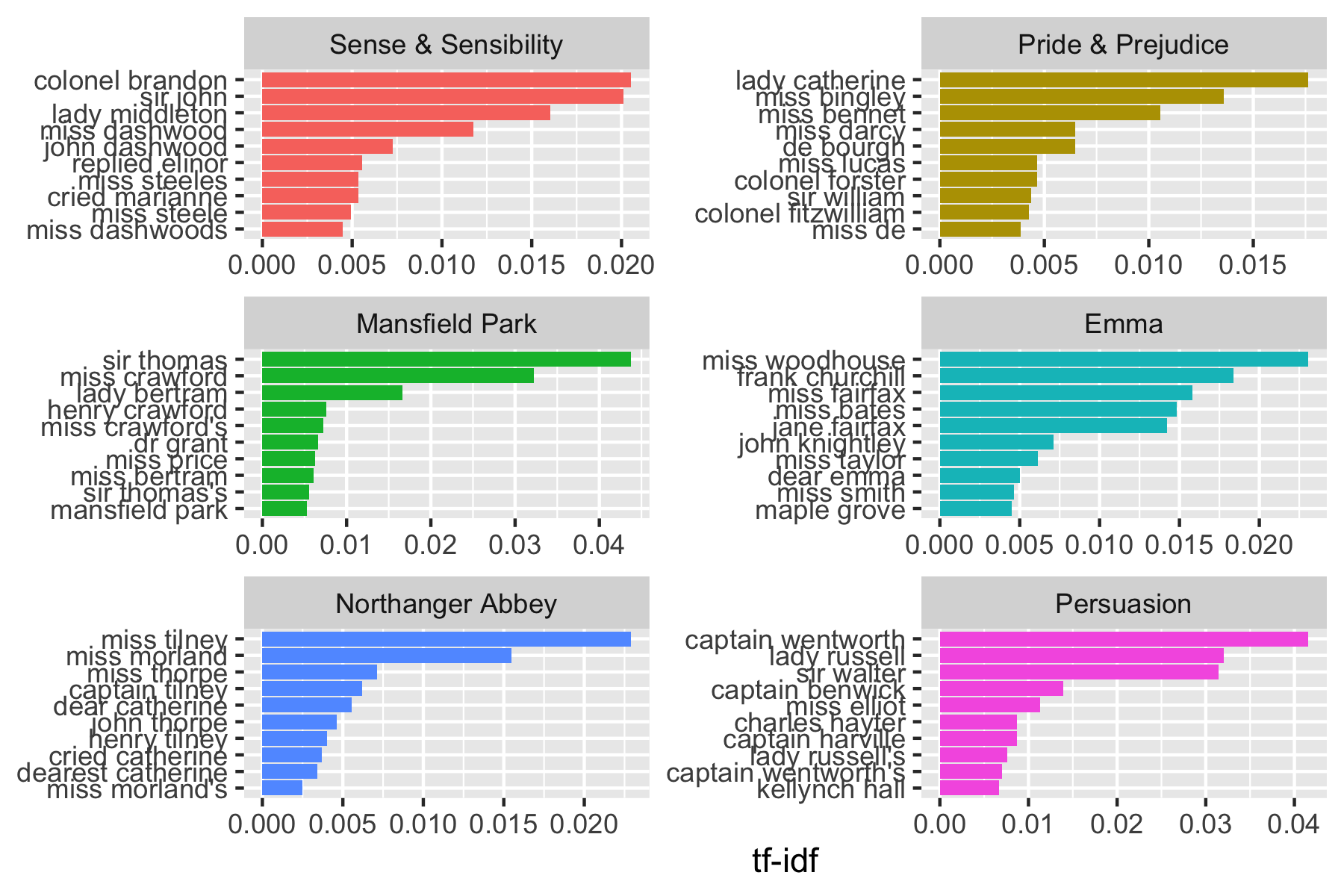

The faceted bar chart above highlights the most distinctive bigrams in each book based on tf-idf.

A heatmap provides a complementary view by placing books and bigrams in a single grid and using color to represent the tf-idf value.

This makes it easier to compare patterns across all books at once and to see which phrases stand out most strongly in particular texts.
We can apply the same idea to both individual words and bigrams, treating each as a term in a document-term matrix.

top_bigrams_heatmap <- bigram_tf_idf |>
  group_by(book) |>
  slice_max(order_by = tf_idf, n = 8) |>
  ungroup()

top_bigrams_heatmap |>
  ggplot(aes(x = book, y = fct_reorder(bigram, tf_idf), fill = tf_idf)) +
  geom_tile(color = "white") +
  scale_fill_viridis_c(end = 0.9) +
  labs(
    title = "Top tf-idf Bigrams Across Jane Austen Books",
    subtitle = "Higher values indicate bigrams that are more distinctive to a given book",
    x = NULL,
    y = NULL,
    fill = "tf-idf"
  ) +
  theme_minimal() +
  theme(axis.text.x = element_text(angle = 45, hjust = 1))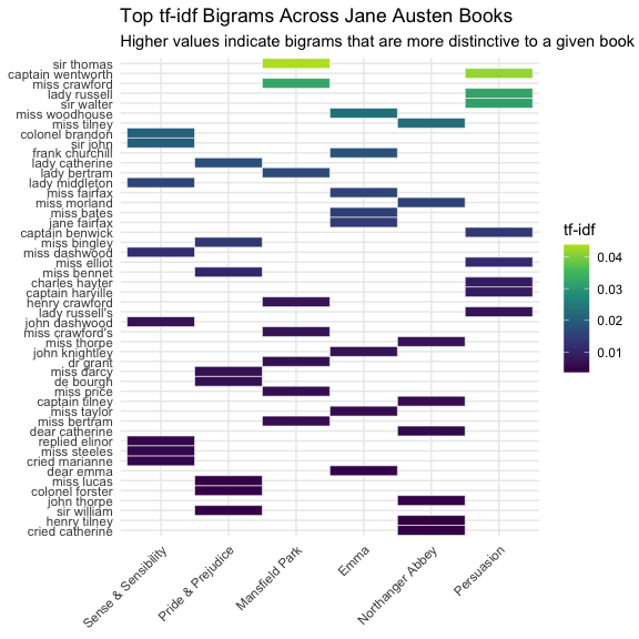

Unlike the faceted bar chart, the heatmap allows us to compare all books and bigrams in one display.

Darker cells indicate bigrams with higher tf-idf values, meaning those phrases are relatively more distinctive to that book than to the others in the collection.

So far, we have used bigrams to identify distinctive phrases. We can also use bigrams to recover local context that is lost in single-word sentiment analysis.

16.3.4 Bigrams in Sentiment Analysis

Per the Readme to the {Sentimentr} package:

English (and other languages) uses Valence Shifters: words that modify the sentiment of other words. Examples include:
- A negator: flips the sign of a polarized word (e.g., “I do not like it.”).
- An amplifier or intensifier increases the impact of a polarized word (e.g., “I really like it.”).
- A de-amplifier or diminisher (downtoner) reduces the impact of a polarized word (e.g., “I hardly like it.”).
- An adversative conjunction overrules the previous clause containing a polarized word (e.g., “I like it but it’s not worth it.”).

These are fairly common in normal usage:

Negators can appear in 20% of sentences with a polarized word.
Adversative conjunctions can appear 10% of the time.
Also see Sentiment Classification of Movie Reviews Using Contextual Valence Shifters

When analyzing at the word level or even sentences, the analysis tends to miss the action of valence shifters.

At a minimum, a negation cancels out a sentiment word so the sentence (or text block) is neutral as opposed to its true, shifted sentiment.

A small step towards improving analysis of sentiment is looking at how often words are preceded by the word “not” on the bigrams.

bigrams_separated |>
  filter(word1 == "not") |>
  count(word1, word2, sort = TRUE)

# A tibble: 1,178 × 3
   word1 word2     n
   <chr> <chr> <int>
 1 not   be      580
 2 not   to      335
 3 not   have    307
 4 not   know    237
 5 not   a       184
 6 not   think   162
 7 not   been    151
 8 not   the     135
 9 not   at      126
10 not   in      110
# ℹ 1,168 more rows

Performing sentiment analysis on the bigram data examines how often sentiment-associated words are preceded by “not” or other negating words.

We could use this to ignore or even reverse their contribution to the sentiment score.

Example: Let’s use the AFINN lexicon (has numeric sentiment values, positive or negative).

library(textdata)
AFINN <- get_sentiments("afinn")
AFINN

# A tibble: 2,477 × 2
   word       value
   <chr>      <dbl>
 1 abandon       -2
 2 abandoned     -2
 3 abandons      -2
 4 abducted      -2
 5 abduction     -2
 6 abductions    -2
 7 abhor         -3
 8 abhorred      -3
 9 abhorrent     -3
10 abhors        -3
# ℹ 2,467 more rows

Find the most frequent words preceded by “not” and associated with a sentiment.

bigrams_separated |>
  filter(word1 == "not") |>
  inner_join(AFINN, by = c(word2 = "word")) |>
  count(word2, value, sort = TRUE) ->
not_words

not_words

# A tibble: 229 × 3
   word2   value     n
   <chr>   <dbl> <int>
 1 like        2    95
 2 help        2    77
 3 want        1    41
 4 wish        1    39
 5 allow       1    30
 6 care        2    21
 7 sorry      -1    20
 8 leave      -1    17
 9 pretend    -1    17
10 worth       2    17
# ℹ 219 more rows

Which words contributed the most in the “wrong” direction?

Let’s multiply their value by the number of times they appear (so a word with a value of +3 occurring 10 times has as much impact as a word with a value of +1 occurring 30 times).

Visualize the result with a bar plot.

not_words |>
  mutate(contribution = n * value) |>
  arrange(desc(abs(contribution))) |>
  head(20) |>
  mutate(word2 = reorder(word2, contribution)) |>
  ggplot(aes(word2, n * value, fill = n * value > 0)) +
  geom_col(show.legend = FALSE) +
  xlab("Words preceded by \"not\"") +
  ylab("Sentiment value * number of occurrences") +
  coord_flip() +
  scale_fill_viridis_d(end = .9)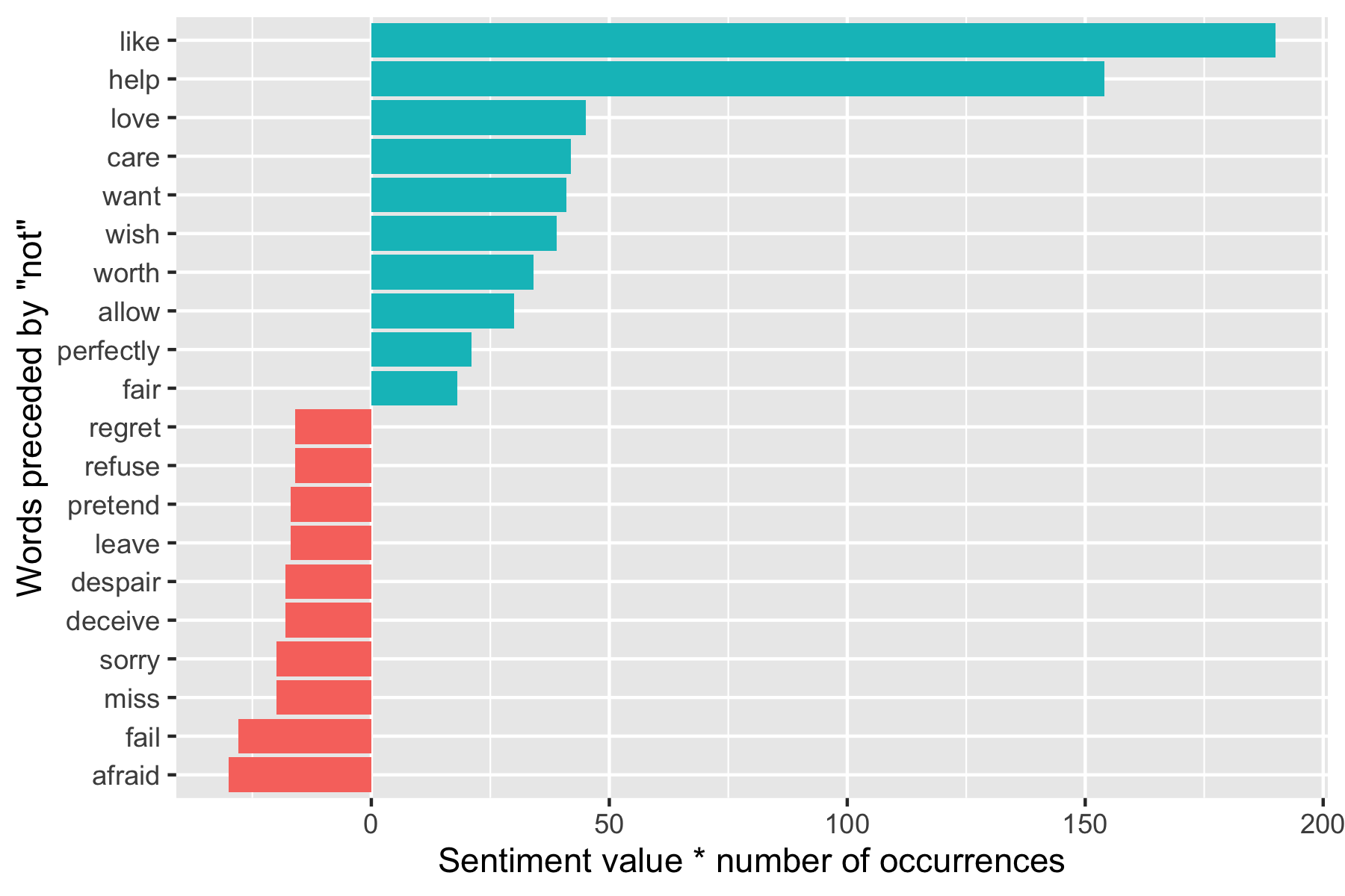

The bigrams “not like” and “not help” make the text seem much more positive than it is.
Phrases like “not afraid” and “not fail” sometimes suggest the text is more negative than it is.
“Not” is not the only word that provides context for the following term.

Let’s pick four common words that negate the subsequent term and use the same joining and counting approach to examine all of them at once.

Note: getting the sort right requires some workarounds.

negation_words <- c("not", "no", "never", "without")

bigrams_separated |>
  filter(word1 %in% negation_words) |>
  inner_join(AFINN, by = c(word2 = "word")) |>
  count(word1, word2, value, sort = TRUE) ->
negated_words

negated_words |>
  mutate(contribution = n * value) |>
  group_by(word1) |>
  slice_max(order_by = abs(contribution), n = 12) |>
  ungroup() |>
  ggplot(aes(reorder_within(word2, contribution, word1), n * value,
    fill = n * value > 0
  )) +
  geom_col(show.legend = FALSE) +
  xlab("Words preceded by negation term") +
  ylab("Sentiment value * Number of Occurrences") +
  coord_flip() +
  facet_wrap(~word1, scales = "free") +
  scale_x_discrete(labels = function(x) str_replace(x, "__.+$", "")) +
  scale_fill_viridis_d(end = .9)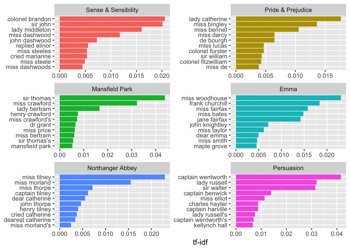

If you want to get more in depth with text analysis, suggest looking at the Readme for the Sentimentr Package.

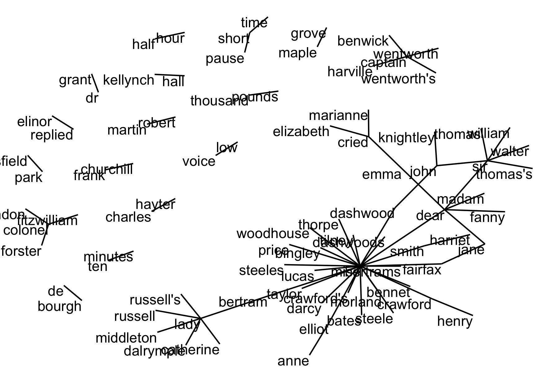
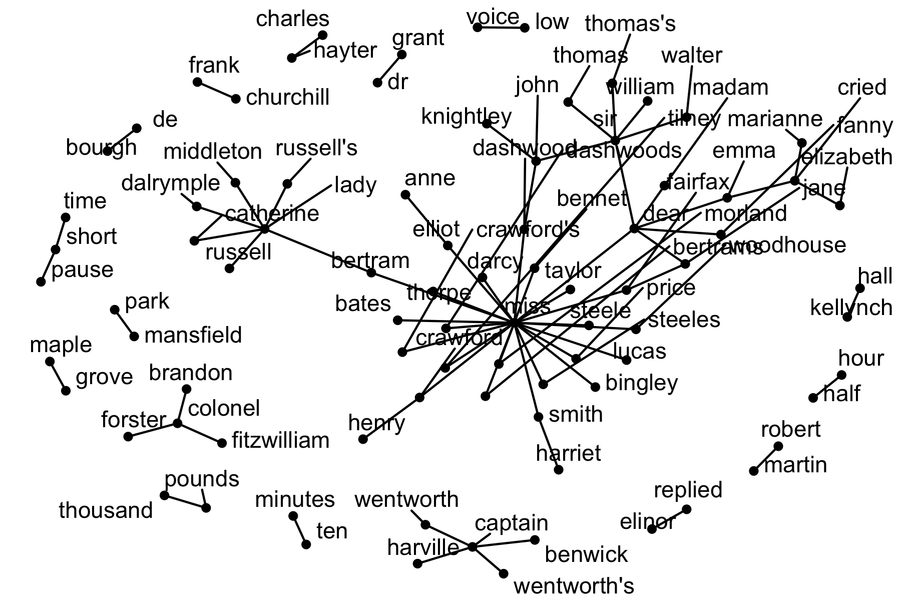
16.3.5 Visualizing a Network of Bigrams with the {igraph} and {ggraph} Packages

If you want to look at more than the top words, you can use a network-node graph to see all of the relationships among words simultaneously.

We can construct a network-node graph from a tidy object since it has three variables with the correct conceptual relationships:

from: the node an edge is coming from,
to: the node an edge is going towards, and
weight: a numeric value associated with each edge.

The {igraph} package is an R package for network analysis.

The main goal of the {igraph} package is to provide a set of data types and functions for

pain-free implementation of graph algorithms,
fast handling of large graphs, with millions of vertices and edges, and
allowing rapid prototyping via high-level languages like R.

One way to create an igraph object from tidy data is to use the graph_from_data_frame() function.

It takes a data frame of edges, with columns for “from”, “to”, and edge attributes (in this case n from our original counts):

Use the console to install {igraph} and then load into the environment.

Take a look at our previously created bigram_counts.

library(igraph)
bigram_counts

# A tibble: 28,975 × 3
   word1   word2         n
   <chr>   <chr>     <int>
 1 <NA>    <NA>      12242
 2 sir     thomas      266
 3 miss    crawford    196
 4 captain wentworth   143
 5 miss    woodhouse   143
 6 frank   churchill   114
 7 lady    russell     110
 8 sir     walter      108
 9 lady    bertram     101
10 miss    fairfax      98
# ℹ 28,965 more rows

Let’s filter out NAs, get the top 20 combinations, and graph.

bigram_counts |>
  filter(n > 20, !is.na(word1), !is.na(word2)) |>
  graph_from_data_frame() ->
bigram_graph

bigram_graph

IGRAPH c9f10b5 DN-- 85 70 -- 
+ attr: name (v/c), n (e/n)
+ edges from c9f10b5 (vertex names):
 [1] sir     ->thomas     miss    ->crawford   captain ->wentworth 
 [4] miss    ->woodhouse  frank   ->churchill  lady    ->russell   
 [7] sir     ->walter     lady    ->bertram    miss    ->fairfax   
[10] colonel ->brandon    sir     ->john       miss    ->bates     
[13] jane    ->fairfax    lady    ->catherine  lady    ->middleton 
[16] miss    ->tilney     miss    ->bingley    thousand->pounds    
[19] miss    ->dashwood   dear    ->miss       miss    ->bennet    
[22] miss    ->morland    captain ->benwick    miss    ->smith     
+ ... omitted several edges

The {ggraph} package is an extension of {ggplot2} tailored to graph visualizations.

It provides the same flexible approach to building up plots layer by layer.

Install with the console and load in this document.

To plot, we need to convert the igraph R object into a ggraph object with the ggraph() function

We then add layers to it (as in ggplot2).

For a basic graph we need to add three layers: nodes, edges, and text.

Given the use of randomized layouts we also set a random number seed for reproducibility.

library(ggraph)
set.seed(17)

ggraph(bigram_graph, layout = "fr") + ##  The Fruchterman-Reingold layout
  geom_edge_link() +
  # geom_node_point() +
  geom_node_text(aes(label = name), vjust = 1, hjust = 1) +
  theme_void()

## With repel = TRUE
set.seed(17)
ggraph(bigram_graph, layout = "fr") + ## The Fruchterman-Reingold layout
  geom_edge_link() +
  geom_node_point() +
  geom_node_text(aes(label = name), vjust = 1, hjust = 1, repel = TRUE) +
  theme_void()

If you want to do more analyses, the {widyr} package helps with other types of bigram analyses to include:

Counting and correlating among sections.
Checking pair-wise correlations.

16.4 Topic Modeling with Latent Dirichlet Allocation (LDA)

We have used term frequency and \(tf-idf\) to identify words that are common or distinctive within documents.

We now turn to a different type of analysis: identifying groups of words that tend to occur together across documents.

Topic modeling Topic modeling is a method for unsupervised classification of documents, similar to clustering on numeric data, which finds natural groups of items even when we’re not sure what we’re looking for. (Silge and Robinson 2025)

The basic assumptions of topic modeling are:

A topic is a collection of words that frequently appear together.
A document is assumed to be a mixture of multiple topics.
Each topic is represented as a probability distribution over words.

Topic modeling helps us explore questions such as:

What themes appear across a collection of documents?
Which words tend to occur together in similar contexts?
How are documents composed of different underlying themes?

Unlike \(tf-idf\), which identifies words that are distinctive to a single document, topic modeling identifies shared structure across documents.

For a survey of multiple methods for topic modeling, see A comprehensive overview of topic modeling: Techniques, applications and challenges (Hankar, Kasri, and Beni-Hssane 2025).

16.4.1 Latent Dirichlet Allocation (LDA)

One of the most common methods for topic modeling is Latent Dirichlet Allocation (LDA).

LDA assumes:

Each document is a mixture of topics.
Each topic is a probability distribution over words.
Different documents may have different mixtures of topics, but some documents may share similar topic distributions.

LDA can be understood as assuming a “generative model” for how documents are created:

For each document, a distribution over topics is drawn.
For each word position in the document:
- A topic is selected from the document’s topic distribution.
- A word is then selected from that topic’s word distribution.

The goal of LDA is to estimate:

The distribution of words within each topic (topic–word distributions), and
The distribution of topics within each document (document–topic distributions).

16.4.1.1 What Does “Latent Dirichlet Allocation” Mean?

The name Latent Dirichlet Allocation reflects how the model is constructed.

Latent means the topics are hidden and must be inferred from the data
Dirichlet refers to a probability distribution used to model how topics and words are distributed
Allocation refers to how words in documents are assigned to topics

More specifically:

Each document has a distribution over topics
Each topic has a distribution over words
These distributions are assumed to follow a Dirichlet distribution, which ensures they are valid probability distributions (non-negative and sum to one)

n practice, we do not observe the topics directly; we only observe the words in the documents.

The model works backward to estimate the hidden (latent) topic structure that most likely generated the observed text.

The Dirichlet distribution

The Dirichlet distribution is used in LDA because it is well-suited for modeling probability distributions over categories.

Topic modeling needs two types of probability distributions:

A distribution of topics within each document, where the categories are the topics.
A distribution of words within each topic where the categories are the words in the vocabulary across all documents.

To be valid probability distributions, they must contain only non-negative values, and sum to 1.

The Dirichlet distribution naturally generates vectors with exactly these properties.

Each draw from a Dirichlet distribution produces a set of proportions (e.g., 0.2, 0.5, 0.3)
These can be interpreted as probabilities over topics or over words
This makes it a natural choice for modeling topic mixtures within documents, and word mixtures within topics

16.4.1.2 Connection to Bayesian Analysis

LDA is a Bayesian model, and the Dirichlet distribution plays the role of a prior distribution.

A prior represents our assumptions about a quantity before seeing the data.
LDA allows us to place Dirichlet priors on:
- the topic distribution for each document, and
- the word distribution for each topic

This provides two important advantages:

Using the Dirichlet distribution ensures all estimated distributions remain valid (non-negative and sum to 1)
It allows us to control the structure and sparsity of the topics

The Dirichlet Distribution also has a key property: it is a conjugate prior for a multinomial distribution.

This means that if we start with a prior distribution \(Dirichlet(α)\) and model observed word counts using a multinomial distribution, then the posterior distribution is also Dirichlet: \(Dirichlet(α+ n)\) where \(n\) represents the observed counts for each category.
- In probability, the multinomial distribution is the natural extension of the binomial distribution (which models two outcomes, such as success/failure) to \(K\) categories

In text analysis, a vocabulary contains many possible words, so word counts in a document follow a multinomial distribution

Words in documents are modeled as draws from this multinomial distribution
The Dirichlet prior combines cleanly with this likelihood

Because of this conjugacy:

Updating the model involves simple count-based adjustments
The posterior remains in the same family as the prior
This makes the mathematics and estimation more tractable

This conjugate structure appears twice in LDA: once for topic distributions within documents, and once for word distributions within topics.

16.4.2 Interpreting the Dirichlet Parameters

The Dirichlet distribution has parameters (often denoted by \(\alpha\) and \(\beta\)) that control how probability mass is distributed.

These parameters influence the structure of the model:

Smaller values (e.g., < 1) encourage sparsity
- Documents concentrate on a few topics
- Topics concentrate on a few words
Larger values (e.g., > 1) produce more even distributions
- Documents mix many topics
- Topics use many words more uniformly

These parameters play a different role than \(K\), the number of topics:

\(K\) determines how many topics exist
\(\alpha\) controls how topics are distributed within documents
\(\beta\) controls how words are distributed within topics

In practice:

\(K\) is chosen directly by the analyst
\(\alpha\) and \(\beta\) are often set to default values or estimated automatically by the model.

16.4.3 Preparing the Data

Topic modeling performs best when working with many smaller documents rather than a few very large ones.

Important

Larger documents (such as full novels) tend to be internally consistent
This can make it difficult for the model to identify distinct topic mixtures
Smaller documents (such as news articles) are more likely to contain varied content

As a result, topic modeling is typically more effective on datasets such as collections of articles.

We will use the Associated Press dataset, which contains thousands of news articles represented as a document-term matrix.

library(topicmodels)
library(tidytext)

data("AssociatedPress", package = "topicmodels")

ap_dtm <- AssociatedPress

ap_dtm

<<DocumentTermMatrix (documents: 2246, terms: 10473)>>
Non-/sparse entries: 302031/23220327
Sparsity           : 99%
Maximal term length: 18
Weighting          : term frequency (tf)

This dataset is already in document-term matrix (DTM) format:

Each row represents a document (news article)
Each column represents a term
Each value is the count of that term in the document

16.4.4 Choosing the Number of Topics K

To fit an LDA model, we must choose the number of topics, denoted by K.

The value of \(K\) determines how many topics the model will try to estimate.

Smaller values of \(K\) produce broader, more general topics
Larger values of \(K\) produce narrower, more specific topics

There is no single “correct” value of \(K\) (although \(K\) is generally much less than the number of documents).

Instead, \(K\) is usually chosen by fitting models with several values and comparing the results.

In practice, we want topics that are:

interpretable
distinct from one another
not so broad that they mix unrelated ideas
not so narrow that they become repetitive or trivial

A useful way to think about this is:

If \(K\) is too small, the topics may be too broad and combine several themes
If \(K\) is too large, the topics may split into overlapping or hard-to-interpret fragments

For this reason, topic modeling is often an iterative process.

We begin with a reasonable range of values for K
We fit a model for each value
We compare the top terms and overall structure of the topics
We then choose a value that provides a useful balance between simplicity and interpretability

16.4.5 Fitting an LDA Model

We will use the LDA() function from {topicmodels} to fit the model.

To fit an LDA model we must choose the number of topics, denoted by \(k\).

For illustration, let’s start with a small value of \(K = 4\) which is small enough to make the initial results easier to interpret.

We also need to set a seed to ensure reproducibility since the model uses random initialization.

lda_fit <- LDA(ap_dtm, k = 4, control = list(seed = 1234))

lda_fit

A LDA_VEM topic model with 4 topics.

The inherent randomness reflects the fact that LDA uses stochastic approximation to estimate a solution, rather than computing a single deterministic result.

Why Do We Set a Random Seed?

LDA uses a randomized, iterative algorithm to assign words to topics and estimate the model.

The algorithm begins by assigning each word to one of the \(k\) topics at random.
It then calculates the probability of each word belonging to each topic based on the current assignments.
It updates these assignments through repeated probabilistic steps.
Different starting assignments can lead to slightly different results.

This is similar to methods like k-means clustering, where random initialization can affect the final solution.

Setting a seed ensures the same random sequence is used each time so the results are reproducible.

Without setting a seed, running the model multiple times may produce different topics or word groupings.

16.4.6 Interpreting the Results from LDA

16.4.6.1 Extracting Topic Information

We can extract the model results using tidy tools.

beta: probability of a word given a topic
gamma: probability of a topic given a document

library(broom)

topics <- tidy(lda_fit, matrix = "beta")
documents <- tidy(lda_fit, matrix = "gamma")

topics

# A tibble: 41,892 × 3
   topic term          beta
   <int> <chr>        <dbl>
 1     1 aaron     2.44e- 5
 2     2 aaron     2.14e- 9
 3     3 aaron     7.30e-12
 4     4 aaron     5.35e- 5
 5     1 abandon   3.52e- 5
 6     2 abandon   7.05e- 5
 7     3 abandon   3.61e- 5
 8     4 abandon   1.22e- 9
 9     1 abandoned 1.27e- 4
10     2 abandoned 2.85e- 5
# ℹ 41,882 more rows

documents

# A tibble: 8,984 × 3
   document topic    gamma
      <int> <int>    <dbl>
 1        1     1 0.000370
 2        2     1 0.238   
 3        3     1 0.000382
 4        4     1 0.000470
 5        5     1 0.172   
 6        6     1 0.0270  
 7        7     1 0.829   
 8        8     1 0.00176 
 9        9     1 0.0132  
10       10     1 0.0698  
# ℹ 8,974 more rows

16.4.6.2 Top Terms in Each Topic

Let’s examine the most important words in each topic.

top_terms <- topics |>
  group_by(topic) |>
  slice_max(beta, n = 10) |>
  ungroup() |>
  mutate(term = reorder_within(term, beta, topic))

top_terms |>
  ggplot(aes(term, beta, fill = factor(topic))) +
  geom_col(show.legend = FALSE) +
  facet_wrap(~topic, scales = "free") +
  coord_flip() +
  scale_x_reordered() +
  scale_fill_viridis_d(end = .9) +
  labs(
    title = "Top Terms in Each Topic",
    x = NULL,
    y = "Probability (beta)"
  )

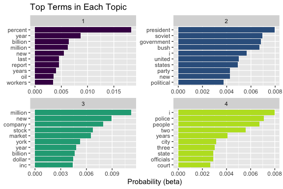
Each panel represents a topic, and the bars show the words most strongly associated with that topic.

Words that appear together in a panel tend to co-occur across documents.
We can interpret each topic by examining these groups of words.

16.4.6.3 Topic Mixtures Within and Across Documents

We can examine how topics are distributed both within individual documents and across the corpus.

This plot shows the topic mixture within a sample of documents.

Some documents are strongly associated with a single topic
Others show a more even mixture of topics

set.seed(1234)
documents |>
  filter(document %in% sample(unique(document), 12)) |>
  ggplot(aes(x = factor(topic), y = gamma, fill = factor(topic))) +
  geom_col(show.legend = FALSE) +
  facet_wrap(~document) +
  labs(
    title = "Topic Mixtures for a Sample of Documents",
    x = "Topic",
    y = "Probability (gamma)"
  ) +
  scale_fill_viridis_d(end = .9)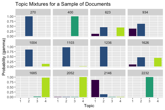

This summary plot shows the number of documents for which each topic is the most likely topic.

Some topics are dominant in more documents than others
This provides a high-level view of how the topics are distributed across the corpus.

documents |>
  group_by(document) |>
  slice_max(gamma, n = 1, with_ties = FALSE) |>
  ungroup() |>
  count(topic) |>
  ggplot(aes(factor(topic), n, fill = factor(topic))) +
  geom_col(show.legend = FALSE) +
  labs(
    title = "Most Likely Topic per Document",
    x = "Topic",
    y = "Number of Documents"
  )

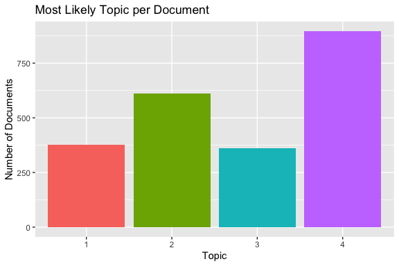
Together, these plots show both the within-document topic mixtures (gamma) and the overall distribution of topics across documents.

16.4.7 Fitting Models for Several Values of K

We will fit several LDA models for the Associated Press dataset and compare the results.

k_values <- c(2, 4, 6, 8) 

lda_models <- map(
  k_values, \(k) LDA(ap_dtm, k = k, control = list(seed = 1234))
)

names(lda_models) <- paste0("k_", k_values)

lda_models

$k_2
A LDA_VEM topic model with 2 topics.

$k_4
A LDA_VEM topic model with 4 topics.

$k_6
A LDA_VEM topic model with 6 topics.

$k_8
A LDA_VEM topic model with 8 topics.

16.4.8 Comparing Topics Across Values of \(K\)

16.4.8.1 Extracting the Top Terms for Each Model

To compare the models, we extract the most probable words in each topic from each fitted model.

top_terms_by_k <- map2_dfr(
  lda_models,
  k_values,
  \(model, k) tidy(model, matrix = "beta") |>
    group_by(topic) |>
    slice_max(beta, n = 8, with_ties = FALSE) |>
    ungroup() |>
    mutate(k = k)
)

top_terms_by_k[top_terms_by_k$topic == 4,]

# A tibble: 24 × 4
   topic term      beta     k
   <int> <chr>    <dbl> <dbl>
 1     4 i      0.00798     4
 2     4 police 0.00710     4
 3     4 people 0.00673     4
 4     4 two    0.00558     4
 5     4 years  0.00407     4
 6     4 city   0.00314     4
 7     4 three  0.00301     4
 8     4 state  0.00292     4
 9     4 i      0.00980     6
10     4 people 0.00536     6
# ℹ 14 more rows

Each row is:

a topic
from a specific model (K value)
with a top term
and its \(\beta\) value

So conceptually, this is:

“For each K, what words define each topic?”

This topic appears to be:

public / civic / reporting language
possibly crime, local reporting, or general news

Why?

police, city, state -> institutional / civic context
people, years -> general reporting language
i, two, three -> noise / general-purpose tokens

Key takeaway

Topics are mixtures of signal + noise
Interpretation comes from identifying the dominant semantic cluster

The top_terms_by_k results show the most probable words (highest \(\beta\) values) for each topic across different values of K.

These results allow us to examine how topic structure changes as the number of topics increases.

Several patterns emerge:

Some topics are stable across different values of \(K\). For example, terms such as percent, million, and billion consistently appear together, indicating a clear economic or financial theme. This suggests that certain topics represent strong underlying structure in the corpus.
As \(K\) increases, broader topics often split into more specific subtopics. For instance, a general “government” topic at lower K may separate into more focused themes such as elections, international relations, or domestic policy at higher K.
Not all topics are equally informative. Some topics contain more generic words such as people, years, or two, which are less useful for interpretation. These topics tend to represent background language rather than distinct themes.
At higher values of \(K\), some topics begin to overlap or repeat similar word patterns, indicating that the model may be over-partitioning the data.

Overall, examining the top terms across values of \(K\) helps assess:

whether topics are coherent,
whether they are distinct from one another, and
whether increasing \(K\) reveals meaningful structure or introduces redundancy.

The top terms across values of \(K\) provide a term-level view of how topics evolve, including which themes are stable, which split into more specific subtopics, and which remain difficult to interpret.

The top terms across values of \(K\) provide an initial view of how topic structure changes as the number of topics increases.

We now visualize these topics to assess their coherence and distinctness, and then examine how topics are distributed across documents to determine whether a given value of \(K\) provides a useful and balanced representation of the corpus.

16.4.8.2 Visualizing the Results

We can now visualize the top terms for each topic across different values of \(K\)

plot_k_topics <- function(k_val) {
  top_terms_by_k |>
    filter(k == k_val) |>
    mutate(
      topic = factor(topic),
      term = reorder_within(term, beta, topic)
    ) |>
    ggplot(aes(term, beta, fill = topic)) +
    geom_col(show.legend = FALSE) +
    facet_wrap(~topic, scales = "free") +
    coord_flip() +
    scale_x_reordered() +
    scale_fill_viridis_d(end = .9) +
    labs(
      title = paste("Top Terms by Topic for K =", k_val),
      x = NULL,
      y = "Probability (beta)"
    ) +
    theme_minimal(base_size = 12) +
    theme(
      axis.text.y = element_text(size = 11),   # word labels
      axis.text.x = element_text(size = 10),   # numeric axis
      strip.text = element_text(size = 11),    # facet titles
      plot.title = element_text(size = 14, face = "bold")
    )
}
walk(k_values, \(k) print(plot_k_topics(k)))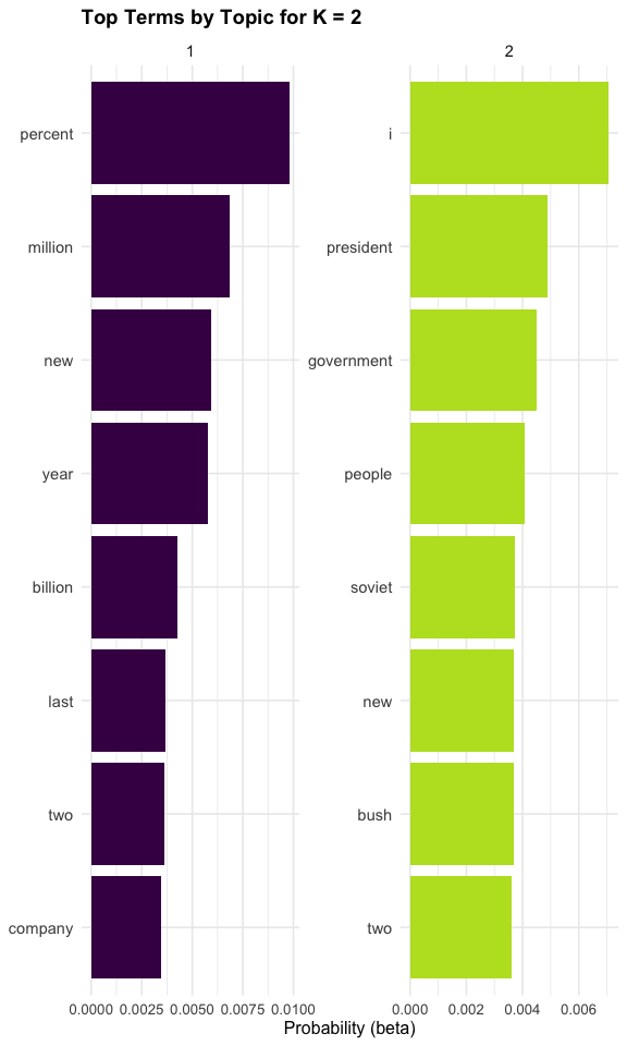

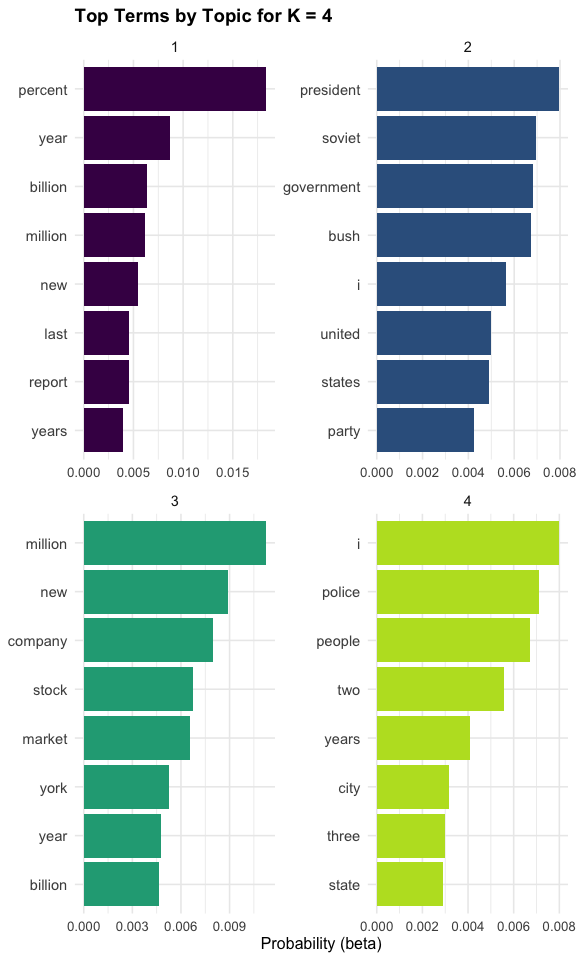
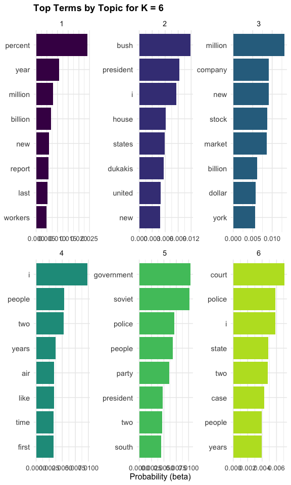
Theses plots helps us compare how the topic structure changes as \(K\) increases.

With smaller values of \(K\), topics are usually broader
With larger values of \(K\), topics are often more specialized
Sometimes larger values of \(K\) reveal useful distinctions
In other cases, they simply split one coherent topic into several similar ones

We can interpret each topic by examining the most probable words associated with it. The goal is not to find a “correct” label, but to identify a coherent theme suggested by the group of words.

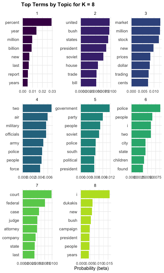
For K = 8, the topics suggest several distinct themes in the Associated Press corpus:

Topic 1 appears to reflect economic indicators and reporting, with words such as percent, year, million, and billion.
Topic 2 reflects U.S. politics and international relations, with terms like united, states, president, and soviet.
Topic 3 clearly represents financial markets, including market, stock, prices, and trading.
Topic 4 captures military and defense, with words such as military, army, officials, and force.
Topic 5 reflects government and political institutions, including government, party, and political.
Topic 6 appears to relate to domestic or social issues, with terms such as police, city, children, and people.
Topic 7 represents the legal system, with words like court, federal, judge, and attorney.
Topic 8 captures elections and political campaigns, including campaign, bush, and dukakis.

Several observations are useful when interpreting these results:

Some broad domains, such as politics, may be split across multiple topics.
For example, Topics 2, 5, and 8 all relate to politics, but capture different aspects:
- international/presidential context,
- general governance, and
- election campaigns.
Topics are not labeled automatically; interpretation requires examining the words and assigning a meaningful theme.
- Small issues in preprocessing can appear in the results.
- For example, the presence of common words such as “i” suggests that additional stop-word filtering could improve the model.

This summary plot shows the number of documents for which each topic is the most likely topic.

Overall, this model produces topics that are:

interpretable,
reasonably distinct, and
aligned with recognizable themes in news data.

This suggests that K = 8 provides a useful level of detail for this corpus, capturing meaningful structure without producing overly broad or overly fragmented topics.

In addition to examining the top terms within each topic, we can also look at how topics are distributed across the corpus.

get_document_distribution <- function(model, k_val) {
  tidy(model, matrix = "gamma") |>
    group_by(document) |>
    slice_max(gamma, n = 1, with_ties = FALSE) |>
    ungroup() |>
    count(topic) |>
    mutate(k = k_val)
}

doc_dist_k8 <- get_document_distribution(lda_models[["k_8"]], 8)

doc_dist_k8 |>
  ggplot(aes(x = factor(topic), y = n, fill = factor(topic))) +
  geom_col(show.legend = FALSE) +
  labs(
    title = "Number of Documents by Dominant Topic (K = 8)",
    x = "Topic",
    y = "Number of Documents"
  ) +
  scale_fill_viridis_d(end = .9)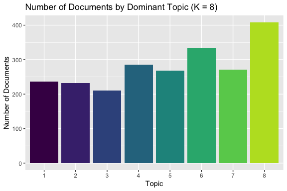

The summary plot shows the number of documents for which each topic is the most likely topic.

The topics are relatively evenly distributed across the corpus.
No topic dominates an overwhelming share of the documents.
No topic is used by only a very small number of documents.

This pattern provides additional support for the choice of K = 8:

The model is not collapsing most documents into just a few broad topics (which would suggest K is too small).
The model is not producing many rarely used or nearly empty topics (which would suggest K is too large).
Instead, the topics appear to represent distinct and reasonably well-used themes in the data.

However, this evidence should be interpreted with caution:

An even distribution of documents across topics does not guarantee that the topics are meaningful or interpretable.
The primary criterion remains whether the top words in each topic form coherent and distinct themes.

Taken together:

The top-term plots suggest that the topics are interpretable and distinct.
The document distribution plot shows that the topics are also broadly used across the corpus.

This combination provides stronger evidence that \(K = 8\) is a reasonable choice for this dataset.

By combining these views, we can make a more informed decision about the number of topics.

The top terms help assess whether topics are coherent and interpretable
The visualizations show whether topics are distinct or overlapping
The document distribution indicates whether topics are meaningfully used across the corpus

An effective choice of \(K\) balances these considerations:

Topics should be interpretable and distinct
Increasing \(K\) should reveal new, meaningful structure, not just split existing topics into redundant fragments
Topics should have reasonable representation across documents, rather than being dominated by only a few or appearing only rarely

In practice, we select the value of \(K\) that provides the clearest and most useful representation of the underlying themes in the corpus, recognizing that topic modeling is an exploratory process rather than a method with a single “correct” answer.

16.4.8.3 How to Compare Models Across Values of \(K\)

After examining the top terms, topic visualizations, and document-level distributions, we can now compare models across different values of \(K\) more systematically.

Rather than relying on a single metric, we evaluate \(K\) based on how well the model captures meaningful structure in the corpus.

Key questions to guide this comparison include:

Topic coherence: Do the top words within each topic form a clear, interpretable theme?
Topic distinctness: Are the topics meaningfully different from one another, or do they overlap?
Added value of increasing \(K\): Does a larger \(K\) reveal new structure, or simply split existing topics into smaller, redundant groups?
Document distribution: Are topics reasonably distributed across documents, or are some topics rarely used or overly dominant?

These criteria reflect a practical reality: interpretability is typically more important than selecting a mathematically “optimal” value of \(K\).

A useful workflow is:

Start with a small value of \(K\)
Increase \(K\) gradually
At each step:
- Examine top terms and topic coherence
- Check for redundancy or fragmentation
- Evaluate how topics are distributed across documents
Stop when increasing \(K\) no longer yields clearer or more meaningful distinctions

In this context:

Smaller values of \(K\) tend to produce broader, more general topics
Larger values of \(K\) tend to produce more detailed, specialized topics

The goal is to find a balance where topics are:

interpretable
distinct
meaningfully represented across the corpus

Once a suitable value of \(K\) is identified, we can focus on that model for deeper interpretation and analysis.

16.4.9 Summary

Topic modeling produces statistical groupings of words, not labeled themes.

Topics must be interpreted by examining their most probable words.
Different choices of \(K\) may produce different topic structures.
Results depend on preprocessing choices such as removing stop words.

Topic modeling is therefore exploratory rather than definitive

It’s useful for identifying patterns, but requires human interpretation

Topic modeling extends our earlier analyses by identifying latent structure in a collection of documents.

\(tf-idf\) identifies words that are distinctive to individual documents.
Topic modeling identifies groups of words that co-occur across documents.
Together, these methods provide complementary perspectives on text data.

Note

Modern approaches to text analysis often use word embeddings and transformer-based models (such as BERT) to capture semantic relationships between words and documents.

These methods can represent meaning more flexibly than \(tf-idf\) or LDA, but they require more advanced tools.

16.5 Converting To and From Non-tidytext Formats

While tidytext format can support a lot of quick analyses, most R packages for NLP are not compatible with this format.

They use sparse matrices for large amounts of text.

However, {tidytext} has functions that allow you to convert back and forth between formats as shown in the Figure 16.1 so you can work with other packages.

Figure 16.1: Tidytext workflows for various formats.

16.5.1 Tidying a document-term matrix (DTM)

One of the most common structures for NLP is the document-term matrix (or DTM).

Each row represents one document (such as a book or article).
Each column represents one term.
Each value (typically) contains the number of appearances of the column term in the row document.

The {tidytext} package provides two functions to convert between DTM and tidytext formats.

tidy() turns a DTM into a tidy data frame. This verb comes from the {broom} package.
cast() turns a tidy one-term-per-row data frame into a matrix.
- cast_sparse() converts to a sparse matrix (from the {Matrix} package),
- cast_dtm() converts to a DTM object (from {tm}),
- cast_dfm() (converts to a dfm object (from {quanteda}).

16.5.2 Tidying Document Term Matrix objects

Perhaps the most widely used implementation of DTMs in R is the DocumentTermMatrix class in the {tm} package.

You can install with the console and load in the document.

Many available text mining datasets are provided in this format.

For example, a collection of Associated Press newspaper articles is in the {topicmodels} package.

library(tm)
data("AssociatedPress", package = "topicmodels")
AssociatedPress

<<DocumentTermMatrix (documents: 2246, terms: 10473)>>
Non-/sparse entries: 302031/23220327
Sparsity           : 99%
Maximal term length: 18
Weighting          : term frequency (tf)

This is a DTM object on which we can use tidytext functions based on the {broom} package to do some format conversions.

Note: documents * terms = 23,522,358 = non-sparse (302031) + number of sparse (23220327)

ap_td <- tidy(AssociatedPress)
ap_td

# A tibble: 302,031 × 3
   document term       count
      <int> <chr>      <dbl>
 1        1 adding         1
 2        1 adult          2
 3        1 ago            1
 4        1 alcohol        1
 5        1 allegedly      1
 6        1 allen          1
 7        1 apparently     2
 8        1 appeared       1
 9        1 arrested       1
10        1 assault        1
# ℹ 302,021 more rows

Note: only the non-zero values are included in the tidied output

We can conduct sentiment analysis as before.

ap_td |>
  inner_join(get_sentiments("bing"), by = c(term = "word")) ->
ap_sentiments

ap_sentiments

# A tibble: 30,094 × 4
   document term    count sentiment
      <int> <chr>   <dbl> <chr>    
 1        1 assault     1 negative 
 2        1 complex     1 negative 
 3        1 death       1 negative 
 4        1 died        1 negative 
 5        1 good        2 positive 
 6        1 illness     1 negative 
 7        1 killed      2 negative 
 8        1 like        2 positive 
 9        1 liked       1 positive 
10        1 miracle     1 positive 
# ℹ 30,084 more rows

And plot as usual.

ap_sentiments |>
  count(sentiment, term, wt = count) |>
  filter(n >= 200) |>
  mutate(n = ifelse(sentiment == "negative", -n, n)) |>
  mutate(term = fct_reorder(term, n)) |>
  ggplot(aes(term, n, fill = sentiment)) +
  geom_bar(stat = "identity") +
  ylab("Contribution to sentiment") +
  coord_flip() +
  scale_fill_viridis_d(end = .9)

16.5.3 Tidying Document-Feature Matrix (DFM) objects

The DFM is an alternative implementation of DTM from the {quanteda} package.

The {quanteda} package comes with a corpus of presidential inauguration speeches, which can be converted to a class dfm object using the appropriate functions.

As of version 3.0, you should tokenize the corpus first.

data("data_corpus_inaugural", package = "quanteda")
library(quanteda)
data_corpus_inaugural |>
  corpus_subset(Year > 1860) |>
  tokens() ->
toks
inaug_dfm <- quanteda::dfm(toks, verbose = FALSE)
inaug_dfm

Document-feature matrix of: 42 documents, 7,930 features (90.58% sparse) and 4 docvars.
               features
docs            fellow-citizens  of the united states : in compliance with  a
  1861-Lincoln                1 146 256      5     19 5 77          1   20 56
  1865-Lincoln                0  22  58      0      0 1  9          0    8  7
  1869-Grant                  0  47  83      3      3 1 27          0   10 19
  1873-Grant                  1  72 106      0      3 2 26          0    9 21
  1877-Hayes                  0 166 240      7     11 0 63          1   19 41
  1881-Garfield               2 181 317      7     15 1 49          0   19 35
[ reached max_ndoc ... 36 more documents, reached max_nfeat ... 7,920 more features ]

The {tidytext} implementation of tidy() works here as well.

inaug_td <- tidy(inaug_dfm)
arrange(inaug_td, term, desc = TRUE)

# A tibble: 31,390 × 3
   document       term  count
   <chr>          <chr> <dbl>
 1 1901-McKinley  "!"       1
 2 1913-Wilson    "!"       1
 3 1937-Roosevelt "!"       1
 4 2009-Obama     "!"       1
 5 1861-Lincoln   "\""     10
 6 1865-Lincoln   "\""      4
 7 1877-Hayes     "\""      2
 8 1881-Garfield  "\""      8
 9 1885-Cleveland "\""      6
10 1889-Harrison  "\""      2
# ℹ 31,380 more rows

We see some punctuation here.

Let’s remove the the terms that are solely punctuation.

inaug_td |> 
  filter(str_detect(term, "^[:punct:]$", negate = TRUE)) ->
  inaug_td

To find words most specific to each of the inaugural speeches we can use tf-idf for each term-speech pair using the bind_tf_idf() function.

inaug_tf_idf <- inaug_td |>
  bind_tf_idf(term, document, count) |>
  arrange(desc(tf_idf))

inaug_tf_idf

# A tibble: 31,125 × 6
   document       term     count      tf   idf tf_idf
   <chr>          <chr>    <dbl>   <dbl> <dbl>  <dbl>
 1 1865-Lincoln   woe          3 0.00429  3.74 0.0160
 2 1865-Lincoln   offenses     3 0.00429  3.74 0.0160
 3 1945-Roosevelt learned      5 0.00898  1.54 0.0138
 4 1961-Kennedy   sides        8 0.00586  2.13 0.0125
 5 1869-Grant     dollar       5 0.00444  2.64 0.0117
 6 1905-Roosevelt regards      3 0.00305  3.74 0.0114
 7 2001-Bush      story        9 0.00568  1.95 0.0111
 8 1945-Roosevelt trend        2 0.00359  3.04 0.0109
 9 1965-Johnson   covenant     6 0.00403  2.64 0.0106
10 1945-Roosevelt test         3 0.00539  1.95 0.0105
# ℹ 31,115 more rows

inaug_tf_idf |>
  filter(document %in% c(
    "1861-Lincoln", "1933-Roosevelt", "1961-Kennedy",
    "2009-Obama", "2017-Trump", "2021-Biden", "2025-Trump"
  )) |>
  mutate(term = str_extract(term, "[a-z']+")) |>
  group_by(document) |>
  arrange(desc(tf_idf)) |>
  slice_max(order_by = tf_idf, n = 10) |>
  ungroup() |>
  ggplot(aes(
    x = reorder_within(term, tf_idf, document),
    y = tf_idf, fill = document
  )) +
  geom_col(show.legend = FALSE) +
  facet_wrap(~document, scales = "free") +
  coord_flip() +
  scale_x_discrete(labels = function(x) str_replace(x, "__.+$", "")) +
  scale_fill_viridis_d(end = .9)

16.5.4 Casting tidy text Data into a Matrix using `cast()`

We can also go the other way: convert tidytext format to a matrix.

Let’s convert the tidied AP dataset back into a DTM using the cast_dtm() function.

ap_td |>
  cast_dtm(document, term, count)

<<DocumentTermMatrix (documents: 2246, terms: 10473)>>
Non-/sparse entries: 302031/23220327
Sparsity           : 99%
Maximal term length: 18
Weighting          : term frequency (tf)

Similarly, we could cast the table into a dfm object from {quanteda} dfm with cast_dfm().

ap_td |>
  cast_dfm(document, term, count)

Document-feature matrix of: 2,246 documents, 10,473 features (98.72% sparse) and 0 docvars.
    features
docs adding adult ago alcohol allegedly allen apparently appeared arrested
   1      1     2   1       1         1     1          2        1        1
   2      0     0   0       0         0     0          0        1        0
   3      0     0   1       0         0     0          0        1        0
   4      0     0   3       0         0     0          0        0        0
   5      0     0   0       0         0     0          0        0        0
   6      0     0   2       0         0     0          0        0        0
    features
docs assault
   1       1
   2       0
   3       0
   4       0
   5       0
   6       0
[ reached max_ndoc ... 2,240 more documents, reached max_nfeat ... 10,463 more features ]

16.5.5 Tidying Corpus Objects with Metadata

The corpus data structure can contain documents before tokenization along with metadata.

For example, the {tm} package comes with the acq corpus, containing 50 articles from the news service Reuters.

data("acq")
acq

<<VCorpus>>
Metadata:  corpus specific: 0, document level (indexed): 0
Content:  documents: 50

A corpus object is structured like a list, with each item containing both text and metadata.

We can use tidy() to construct a table with one row per document, including the metadata (such as id and datetimestamp) as columns alongside the text.

acq_td <- tidy(acq)
acq_td

# A tibble: 50 × 16
   author   datetimestamp       description heading id    language origin topics
   <chr>    <dttm>              <chr>       <chr>   <chr> <chr>    <chr>  <chr> 
 1 <NA>     1987-02-26 15:18:06 ""          COMPUT… 10    en       Reute… YES   
 2 <NA>     1987-02-26 15:19:15 ""          OHIO M… 12    en       Reute… YES   
 3 <NA>     1987-02-26 15:49:56 ""          MCLEAN… 44    en       Reute… YES   
 4 By Cal … 1987-02-26 15:51:17 ""          CHEMLA… 45    en       Reute… YES   
 5 <NA>     1987-02-26 16:08:33 ""          <COFAB… 68    en       Reute… YES   
 6 <NA>     1987-02-26 16:32:37 ""          INVEST… 96    en       Reute… YES   
 7 By Patt… 1987-02-26 16:43:13 ""          AMERIC… 110   en       Reute… YES   
 8 <NA>     1987-02-26 16:59:25 ""          HONG K… 125   en       Reute… YES   
 9 <NA>     1987-02-26 17:01:28 ""          LIEBER… 128   en       Reute… YES   
10 <NA>     1987-02-26 17:08:27 ""          GULF A… 134   en       Reute… YES   
# ℹ 40 more rows
# ℹ 8 more variables: lewissplit <chr>, cgisplit <chr>, oldid <chr>,
#   places <named list>, people <lgl>, orgs <lgl>, exchanges <lgl>, text <chr>

We can then unnest_tokens(), for example, to find the most common words across the 50 Reuters articles.

acq_tokens <- acq_td |>
  select(-places) |>
  unnest_tokens(word, text) |>
  anti_join(stop_words, by = "word")

## most common words
acq_tokens |>
  count(word, sort = TRUE)

# A tibble: 1,566 × 2
   word         n
   <chr>    <int>
 1 dlrs       100
 2 pct         70
 3 mln         65
 4 company     63
 5 shares      52
 6 reuter      50
 7 stock       46
 8 offer       34
 9 share       34
10 american    28
# ℹ 1,556 more rows

Or the words most specific to each article (by id).

## tf-idf
acq_tokens |>
  count(id, word) |>
  bind_tf_idf(word, id, n) |>
  arrange(desc(tf_idf))

# A tibble: 2,853 × 6
   id    word         n     tf   idf tf_idf
   <chr> <chr>    <int>  <dbl> <dbl>  <dbl>
 1 186   groupe       2 0.133   3.91  0.522
 2 128   liebert      3 0.130   3.91  0.510
 3 474   esselte      5 0.109   3.91  0.425
 4 371   burdett      6 0.103   3.91  0.405
 5 442   hazleton     4 0.103   3.91  0.401
 6 199   circuit      5 0.102   3.91  0.399
 7 162   suffield     2 0.1     3.91  0.391
 8 498   west         3 0.1     3.91  0.391
 9 441   rmj          8 0.121   3.22  0.390
10 467   nursery      3 0.0968  3.91  0.379
# ℹ 2,843 more rows

16.5.6 Format Conversion Summary

Text analysis requires working with a variety of tools, many of which use non-tidytext formats.

You can use tidytext functions to convert between a tidy text data frame and other formats such as DTM, DFM, and Corpus objects containing document metadata to facilitate your own work or collaboration with others.

16.6 Responsible Data Science in Text Analysis

Text data often contains rich contextual information, but it can also include sensitive information or use methods and tools suggest the need for careful consideration of both ethical use and interpretability of results.

16.6.1 Privacy and Personally Identifiable Information (PII)

Text data frequently contains information from or about individuals as part of free-form text as opposed to specific fields in a structured dataset.

Personally identifiable information (PII) can be direct or indirect.

Direct PII: names, addresses, phone numbers, and email addresses may appear explicitly
Indirect identifiers: e.g., job titles, locations, unique events can enable re-identification
Even when obvious identifiers are removed, contextual clues may still reveal identities

This creates several risks:

Unintentional disclosure of sensitive information
Re-identification from seemingly anonymized text
*Bias amplification** if certain groups are more identifiable or over-represented

Common mitigation strategies include:

Removing or masking PII using rule-based or model-based approaches.
Aggregating data to higher levels (e.g., document summaries instead of raw text)
Limiting access to raw text and using secure data environments
Applying differential privacy or synthetic data generation where appropriate

Important

Text data should be treated as high-risk data from a privacy perspective, even when it appears unstructured or anonymized.

16.6.1.1 Examples: Removing or Masking PII in Text Data

16.6.1.1.1 Rule-Based Approaches (Deterministic, Pattern Matching).

These rely on predefined patterns such as regular expressions or lookup dictionaries.

Example: Masking email addresses and phone numbers

text <- "Contact John at john.doe@email.com or 202-555-1234."

text |>
  stringr::str_replace_all("[A-Za-z0-9._%+-]+@[A-Za-z0-9.-]+", "[EMAIL]") |>
  stringr::str_replace_all("\\b\\d{3}-\\d{3}-\\d{4}\\b", "[PHONE]")

[1] "Contact John at [EMAIL] or [PHONE]."

Example: Masking names using a lookup list

names_list <- c("John", "Mary", "Smith")
text <- "John Smith submitted the report."
text |>
  stringr::str_replace_all(stringr::str_c(names_list, collapse = "|"), "[NAME]")

[1] "[NAME] [NAME] submitted the report."

These approaches are fast, transparent, and easy to implement for structured PII (emails, SSNs, phone numbers).

However, they can miss variations and context (e.g., unusual formats), requires a lot of manual rule maintenance and cannot reliably detect ambiguous entities (e.g., “Jordan” a name versus “Jordan” the country).

16.6.1.1.2 Model-Based Approaches (Context-Aware, NLP Models)

These use Named Entity Recognition (NER) models to detect entities such as people, locations, and organizations.

Example: Using an NLP model from {spacyr} to detect and mask entities.

Note {spacyr} is a wrapper for the python {spaCy} library, which provides pre-trained models for natural language processing including NER.
See the documentation to install the package and then install the underlying python.

text <- "John Smith works at Acme Corp in Washington and his email is john.smith@email.com."

# Run Named Entity Recognition
entities <- spacyr::spacy_extract_entity(text)

entities

  doc_id                 text ent_type start_id length
1  text1           John Smith   PERSON        1      2
2  text1            Acme Corp      ORG        5      2
3  text1           Washington      GPE        8      1
4  text1 john.smith@email.com      ORG       13      1

Note: “GPE is”Geo-Political Entity”, which includes locations such as cities and countries.

Now that you have the elements of interest, you can mask them in the original text.

A nice use case for purr::reduce() to iteratively replace each entity with its type in the text and return the string.
Using stringr::fixed() ensures each entity is treated as a literal string, not a regular expression, so special characters (e.g., periods in emails or titles like “Dr. Smith”) are matched exactly and do not produce unintended replacements.
When replacing entities detected by NLP models, using literal string matching (e.g., fixed()) helps to avoid unintended matches caused by regex special characters in the text.

library(stringr)
library(purrr)

masked_text <- reduce(
  seq_len(nrow(entities)),
  \(txt, i) {
    str_replace_all(
      txt,
      fixed(as.character(entities$text[i])),
      paste0("[", entities$ent_type[i], "]")
    )
  },
  .init = text
)

masked_text

[1] "[PERSON] works at [ORG] in [GPE] and his email is [ORG]."

As you can see, the {spaCy} models do not always reliably detect emails, so you can add another step using regular regex:

masked_text |>
  stringr::str_replace_all(
    "[A-Za-z0-9._%+-]+@[A-Za-z0-9.-]+",
    "[EMAIL]"
  )

[1] "[PERSON] works at [ORG] in [GPE] and his email is [ORG]."

The NER approach captures context (names, organizations, locations) and is more flexible than rules, especially for unstructured text.

However, they are probabilistic so may miss or misclassify entities.
They may also require model selection and tuning.
They are less transparent than rule-based methods

Hybrid Approach: In practice, combining both approaches is often most effective.

Example workflow:

Apply regex rules for: Emails, Phone numbers and IDs 2. Apply NER model for: Names, Locations, and Organizations 3. Post-process to normalize tags (e.g., [PERSON], [ORG]) and review edge cases

Important

Results are probabilistic, errors and missed entities are inevitable.
Removing explicit identifiers does not guarantee anonymity.
Even after masking explicit PII, contextual information in text can still enable re-identification, especially in small or specialized datasets.
Always validate results, especially when working with sensitive data.

16.6.2 Explainability and Responsible AI in Text Analysis

As models become more complex, understanding and communicating their behavior becomes increasingly important.

16.6.2.1 Interpreting Model Outputs vs Explaining Decisions

It is important to distinguish between:

Interpretation: understanding patterns in model outputs
Explanation: understanding why a specific prediction or decision was made

For example:

In LDA, we interpret topics by examining high-probability words
In classification models, we explain why a document was labeled a certain way

These are related but fundamentally different tasks.

16.6.3 Limits of Statistical Interpretability

Models like Latent Dirichlet Allocation provide interpretable outputs, but this interpretability has limits.

Topics are statistical groupings of co-occurring words, not causal mechanisms
A topic does not “explain” why words occur, it summarizes patterns in the text.
Interpretations are human-imposed labels on probabilistic structures

This distinction is critical:

LDA provides descriptive structure, not causal insight.
Misinterpreting topics as explanations can lead to incorrect conclusions.

16.6.3.1 Comparison with Modern Black-Box Models

More recent approaches to text analysis, such as transformer-based models like BERT, offer improved performance but reduced transparency.

Key differences:

LDA:
- Transparent structure (topics and word distributions)
- Easier to interpret but less expressive
Transformer models:
- Capture complex semantic relationships
- Often considered black-box models
- Harder to interpret directly

This creates a trade-off of Interpretability vs predictive power

16.6.3.2 Tools for Model Explanation

To address the lack of transparency in complex models, several tools have been developed:

[LIME]{https://christophm.github.io/interpretable-ml-book/lime.html)
- Explains individual predictions using local approximations
- Helps identify which features (e.g., words) influenced a decision
SHAP (SHapley Additive exPlanations)
- Based on game theory for allocating “payouts” for feature importance.
- Provides consistent feature importance values across predictions
Attention analysis (in transformer models)
- Examines which words (tokens) influence the model outputs.
- Provides insight into internal weighting, though not always a true explanation

Each of these methods has limitations:

They provide approximations, not definitive explanations or ground truth.
Results can vary depending on model and configuration
Interpretations still require human judgment

16.6.4 Practical Guidance for Responsible Text Analysis

When applying text analysis methods:

Be explicit about what the model can and cannot explain
Avoid presenting statistical patterns as causal findings
Evaluate whether the level of interpretability is appropriate for the application
Consider the ethical implications of using sensitive or identifiable text data
Document your preprocessing, modeling choices, and limitations clearly

16.6.5 Summary

Responsible text analysis requires attention to both data ethics and model transparency.

Text data introduces unique privacy and re-identification risks.
Interpretable models like LDA provide useful structure but not causal explanations.
More powerful models increase the need for post hoc explanation tools.
Clear communication of limitations is essential for responsible use.

16.1 Introduction

16.1.1 Learning Outcomes

16.1.2 References:

16.1.2.1 Other References

16.2 Identifying Important Terms in a Corpus

16.2.1 Term Frequency - Inverse Document Frequency (tf-idf)

16.2.1.1 TF in Jane Austen’s Novels

16.2.1.2 Background on Zipf’s Law

16.2.1.3 Zipf’s law for Jane Austen

16.2.2 Applying \(tf-idf\) to a Corpus

16.2.2.1 Example: Using tf-idf to Analyze a Corpus of Physics Texts

16.2.3 TF-IDF Summary

16.3 Relationships Between Words: Analyzing n-Grams

16.3.1 Tokenizing by n-gram

16.3.2 Counting and filtering n-Grams

16.3.3 Analyzing bigrams

16.3.4 Bigrams in Sentiment Analysis

16.3.5 Visualizing a Network of Bigrams with the {igraph} and {ggraph} Packages

16.4 Topic Modeling with Latent Dirichlet Allocation (LDA)

16.4.1 Latent Dirichlet Allocation (LDA)

16.4.1.1 What Does “Latent Dirichlet Allocation” Mean?

16.4.1.2 Connection to Bayesian Analysis

16.4.2 Interpreting the Dirichlet Parameters

16.4.3 Preparing the Data

16.4.4 Choosing the Number of Topics K

16.4.5 Fitting an LDA Model

16.4.6 Interpreting the Results from LDA

16.4.6.1 Extracting Topic Information

16.4.6.2 Top Terms in Each Topic

16.4.6.3 Topic Mixtures Within and Across Documents

16.4.7 Fitting Models for Several Values of K

16.4.8 Comparing Topics Across Values of \(K\)

16.4.8.1 Extracting the Top Terms for Each Model

16.4.8.2 Visualizing the Results

16.4.8.3 How to Compare Models Across Values of \(K\)

16.4.9 Summary

16.5 Converting To and From Non-tidytext Formats

16.5.1 Tidying a document-term matrix (DTM)

16.5.2 Tidying Document Term Matrix objects

16.5.3 Tidying Document-Feature Matrix (DFM) objects

16.5.4 Casting tidy text Data into a Matrix using cast()

16.5.5 Tidying Corpus Objects with Metadata

16.5.6 Format Conversion Summary

16.6 Responsible Data Science in Text Analysis

16.6.1 Privacy and Personally Identifiable Information (PII)

16.6.1.1 Examples: Removing or Masking PII in Text Data

16.6.1.1.1 Rule-Based Approaches (Deterministic, Pattern Matching).

16.6.1.1.2 Model-Based Approaches (Context-Aware, NLP Models)

16.6.2 Explainability and Responsible AI in Text Analysis

16.6.2.1 Interpreting Model Outputs vs Explaining Decisions

16.6.3 Limits of Statistical Interpretability

16.6.3.1 Comparison with Modern Black-Box Models

16.6.3.2 Tools for Model Explanation

16.6.4 Practical Guidance for Responsible Text Analysis

16.6.5 Summary

16.5.4 Casting tidy text Data into a Matrix using `cast()`