[1] "am a" "4" 3 Tidyverse Review
Keywords
Tidyverse, stringr, regex, lubridate, forcats
3.1 Introduction
3.1.1 Learning Outcomes
- Manipulate strings with the {stringr} package.
- Employ regular expressions (REGEX or regex) with strings.
- Manipulate dates and times using the {lubridate} package.
- Manipulate factors using the {forcats} package.
- Employ current capabilities of Tidyverse packages to deliver data science solutions.
- Employ literate programming as part of responsible data science.
3.1.2 References:
- R for Data Science 2nd Edition Wickham et al. (2023)
- {stringr} package Wickham (2022)
- {stringr} Vignette on Regular Expressions
- {lubridate} package Grolemund and Wickham (2011)
- {forcats} package Wickham (2023)
- {tidyverse} package Wickham et al. (2019)
- Quarto Posit (2022)
3.1.2.1 Other References
3.2 Strings
- In R, strings (also called “characters”) are created and displayed within quotes.
- Anything within quotes is a string, even numbers or punctuation.
- You can have a vector of strings and use the subset operator
[...].
- You can use special characters in strings using the “escape character”
\which indicates the character after the backslash is to be treated as a special character. - For example, if you want to put a quotation mark in a string, you must “escape” the quotation mark with a backslash.
As Tolkien said, "Not all those who wander are lost"[1] "As Tolkien said, \"Not all those who wander are lost\"""\n"means create a new line.
- If you want to indicate a
\, you must escape it, so use two\\.
3.2.1 The {stringr} Package
- The {stringr} package has functions to make manipulating strings easier - (more user-friendly than base R’s
grep()andgsub()). - {stringr} loads with the {tidyverse}.
- All {stringr} functions begin with
str_so in RStudio you can press tab after typingstr_to show a list of possible string manipulation functions. - The {stringr} functions we will cover today are often useful in cleaning or analyzing data from the web or during text analysis.
- Many {stringr} functions have a
pattern =argument where the pattern describes a string of interest that one is trying to match.- The pattern is often described using a “regular expression”. We will review these later.
- Simple patterns can use just letters and operators such as
|for OR.
3.2.1.1 Detect Matches
str_detect(string, pattern): Returns a logical value or vector:TRUEfor a match to the pattern andFALSEif no match is found.- The
negate =argument reverses the result.
- The
- Useful for creating new variables or filtering rows.
# A tibble: 12 × 5
   name       start      end        party      has_a_e
   <chr>      <date>     <date>     <chr>      <lgl>
 1 Eisenhower 1953-01-20 1961-01-20 Republican TRUE
 2 Kennedy    1961-01-20 1963-11-22 Democratic TRUE
 3 Johnson    1963-11-22 1969-01-20 Democratic FALSE
 4 Nixon      1969-01-20 1974-08-09 Republican FALSE
 5 Ford       1974-08-09 1977-01-20 Republican FALSE
 6 Carter     1977-01-20 1981-01-20 Democratic TRUE
 7 Reagan     1981-01-20 1989-01-20 Republican TRUE
 8 Bush       1989-01-20 1993-01-20 Republican FALSE
 9 Clinton    1993-01-20 2001-01-20 Democratic FALSE
10 Bush       2001-01-20 2009-01-20 Republican FALSE
11 Obama      2009-01-20 2017-01-20 Democratic TRUE
12 Trump 2017-01-20 2021-01-20 Republican FALSE # A tibble: 5 × 4
name start end party
<chr> <date> <date> <chr>
1 Eisenhower 1953-01-20 1961-01-20 Republican
2 Kennedy 1961-01-20 1963-11-22 Democratic
3 Carter 1977-01-20 1981-01-20 Democratic
4 Reagan 1981-01-20 1989-01-20 Republican
5 Obama 2009-01-20 2017-01-20 Democratic# A tibble: 7 × 4
name start end party
<chr> <date> <date> <chr>
1 Johnson 1963-11-22 1969-01-20 Democratic
2 Nixon 1969-01-20 1974-08-09 Republican
3 Ford 1974-08-09 1977-01-20 Republican
4 Bush 1989-01-20 1993-01-20 Republican
5 Clinton 1993-01-20 2001-01-20 Democratic
6 Bush 2001-01-20 2009-01-20 Republican
7 Trump 2017-01-20 2021-01-20 Republicanstr_count(string, pattern): Counts the number of matches within a string.
# A tibble: 12 × 2
   name       count
   <chr>      <int>
 1 Eisenhower     2
 2 Kennedy        2
 3 Johnson        0
 4 Nixon          0
 5 Ford           0
 6 Carter         2
 7 Reagan         3
 8 Bush           0
 9 Clinton        0
10 Bush           0
11 Obama          2
12 Trump 0str_count()counts non-overlapping matches.
3.2.1.2 Subset Strings
str_sub(string, start, end)extracts the substring between the location of two characters (inclusive).- Default values for
startandendare1Land-1L.
[1] "The Road goes ever on and on"[1] "e Road goes ever on and on"[1] "The Ro"[1] "e Ro"- You can also use
str_sub()to replace substrings by assignment.
str_subset(string, pattern, negate)returns the strings where there is a match.negate = TRUEreturns those without a match.
3.2.1.3 Manage Lengths
str_length(string)returns the count of “characters” (including spaces and punctuation).- Special characters, starting with the escape symbol
\, only count as 1 character.
[1] 21[1] 22[1] 24[1] 25str_trim(string, side)removes (potentially troublesome) invisible white space on the beginning and/or the end of a string.str_squish(string)removes invisible spaces at the beginning and end, and also collapses multiple spaces in the middle of a string into one space.- Extra spaces can happen a lot with human-entered data.
[1] " This is a string with extra whitespaces in the beginning, middle and end. "[1] "This is a string with extra whitespaces in the beginning, middle and end."[1] "This is a string with extra whitespaces in the beginning, middle and end."3.2.1.4 Mutate Strings - Change the Characters in a String
3.2.1.4.1 Extracting/Assigning Substrings (Parts of a String)
As seen in Section 3.2.1.2,
str_sub()can mutate a string by extracting a substring located between two characters (inclusive) or assigning new values to a substring.str_replace()andstr_replace_all()will replace matched patterns with the provided strings.str_replace(string, pattern, replacement)replaces just the first match to the pattern in a string with the replacement stringstr_replace_all(string, pattern, replacement)replaces all matched patterns.
Example: we want to get rid of all punctuation in the following phrase (the
|means “OR”). Notice we have to escape the period.and!with\\.
Farewell we call to hearth and hall!
Though wind may blow and rain may fall,
We must away ere break of day
Far over wood and mountain tall.[1] "Farewell we call to hearth and hall \nThough wind may blow and rain may fall\nWe must away ere break of day\nFar over wood and mountain tall"str_to_lower(string)andstr_to_upper(string)convert all letters to lower or capital case.str_to_sentenceconverts all words and letters to sentence case, even acronyms.
[1] "Deeds will Not be LESS vaLiant in the USA because THey are unpraised."[1] "deeds will not be less valiant in the usa because they are unpraised."[1] "DEEDS WILL NOT BE LESS VALIANT IN THE USA BECAUSE THEY ARE UNPRAISED."[1] "Deeds will not be less valiant in the usa because they are unpraised."[1] "Deeds will not be less valiant in the USA because they are unpraised."3.2.1.5 Join and Split Strings
3.2.1.5.1 Joining Strings
- Combine/concatenate strings with
str_c(..., sep = "", collapse = NULL).
[1] "Faithless is he that saysfarewell when the road darkens."- The default is to separate strings by nothing. Use the
separgument to change the separator.
- If you provide
str_c()a vector of arguments, it will vectorize the combining to include recycling the shorter argument. - You can provide a
collapse =argument to convert to a single string from a vector. - Also see help for
str_flatten().
[1] "Short" "cuts" "make" "long" "delays."[1] "Short-LOTR" "cuts-LOTR" "make-LOTR" "long-LOTR" "delays.-LOTR"[1] "Short cuts make long delays."[1] "ShortLOTR cutsLOTR makeLOTR longLOTR delays.LOTR"- Combining with
NAresults inNA:
3.2.1.6 Joining Strings with Values from Variables or Functions
str_glue(..., .sep)is a wrapper around theglue::glue()function which allows you to “interpolate” strings and variables, e.g., combine a string with the dynamic value of a variable.- Notice the argument is
.sepnotsep
- Notice the argument is
- This can be useful in in-line code and text elements in graphics as an alternative to
paste()andpaste0().
3.2.1.7 Split a String into Multiple Strings
str_split()will split a string based on a character we choose; useful with dates or full names at times.- Can help simplify working with long strings by breaking them into shorter pieces for analysis.
- By default, the output is a list. Have to be careful when the string could split into different numbers of elements.
3.2.1.8 Split a Data Frame Column of Type Character with separate()
The
separate()function, from the {tidyr} package, is useful for splitting all the strings in a data frame column into multiple columns.You can use regex or a vector of positions to turn a single column into multiple columns.
You need to specify at least three arguments:
- The column you want to separate that has two (or more) variables,
- The character vector of the names of the new variables, and
- The character or numeric positions by which to separate out the new variables from the current column.
Consider {tidyr}’s table three which has cases and country population combined.
# A tibble: 6 × 3
  country      year rate
  <chr>       <dbl> <chr>
1 Afghanistan  1999 745/19987071
2 Afghanistan  2000 2666/20595360
3 Brazil       1999 37737/172006362
4 Brazil       2000 80488/174504898
5 China        1999 212258/1272915272
6 China 2000 213766/1280428583# A tibble: 6 × 4
country year cases population
<chr> <dbl> <chr> <chr>
1 Afghanistan 1999 745 19987071
2 Afghanistan 2000 2666 20595360
3 Brazil 1999 37737 172006362
4 Brazil 2000 80488 174504898
5 China 1999 212258 1272915272
6 China 2000 213766 1280428583- See also
tidyr::extract().
The separate() function has recently been superseded by three new functions in {tidyr}.
separate_wider_delim()splits by delimiter.separate_wider_position()splits at fixed widths.separate_wider_regex()splits with regular expression matches.
# A tibble: 6 × 4
  country      year cases  population
  <chr>       <dbl> <chr>  <chr>
1 Afghanistan  1999 745    19987071
2 Afghanistan  2000 2666   20595360
3 Brazil       1999 37737  172006362
4 Brazil       2000 80488  174504898
5 China        1999 212258 1272915272
6 China 2000 213766 12804285833.2.2 Regular Expressions
3.2.2.1 Intro
- Regular expressions (regex or regexp) are a syntax for pattern matching in strings.
- Regex syntax is used by programmers in many computer languages. There are some slight variations but most uses are the same.
- Wherever there is a
patternargument in a {stringr} function, you can use regex (to extract strings, get a logical if there is a match, etc.).
3.2.2.2 Regex Match Characters and Escaping with the Backslash \
Regex syntax includes special “match characters”, e.g.,
.,?,(,),", and\.These must be escaped using
\if you want to match their normal value.Then you must also escape the
\so always use two\\in front of a match character as stated on the Cheat Sheet.Basic usage: find exact match(es) of a string pattern and replace them with the designated replacement string.
[1] "Ho! Ho! Ho! to the bottle I go to XXl my XXrt and drown my woe."- A period “
.” matches any character to include spaces and punctuation.
[1] "Ho! Ho! Ho! to the bottle I go to XX my XXt and drown my woe."- You “escape” a period with two backslashes “
\\.” to match actual periods in the text. - You can also use match characters in the replacement string.
[1] "XXXXXXXXXXXXXXXXXXXXXXXXXXXXXXXXXXXXXXXXXXXXXXXXXXXXXXXXXXXXXXXXX"[1] "Ho! Ho! Ho! to the bottle I go to heal my heart and drown my woeX"[1] "Ho! Ho! Ho! to the bottle I go to heal my heart and drown my woe?"[1] "Ho, Ho, Ho, to the bottle I go to heal my heart and drown my woe."- To match an escaped backslash
\\, you need four backslashes (to escape the escape twice).
Rain and\or snow may fall and\or blow[1] "Rain and\\or snow may fall and\\or blow"[1] "Rain andXXor snow may fall andXXor blow"3.2.2.3 Other Regex Match Characters Serve as “Wild Cards”
- These each have a negated value by using the capital letter in the syntax.
- We’ll use this character vector for practice:
\\dmatches any digit,\\Dany non-digit.
[1] "Abba: XXX-XXXX" "Ann: XXX-XXXX" "Andy_R: XXX-XXXX"[1] "XXXXXX555X1234" "XXXXX555X0987" "XXXXXXXX555X7654"\\smatches any white space (e.g. space, tab, newline),\\Sany non-white space.
[1] "Abba: 555-1234" "Ann: 555-0987" "Andy_R: 555-7654"[1] "Abba:X555-1234" "Ann:X555-0987" "Andy_R:X555-7654"[1] "XXXXX XXXXXXXX" "XXXX XXXXXXXX" "XXXXXXX XXXXXXXX"\\wmatches any word character (letter, digit, or underscore),\\Wany non-word character.
[1] "Abba: 555-1234" "Ann: 555-0987" "Andy_R: 555-7654"[1] "XXXX: XXX-XXXX" "XXX: XXX-XXXX" "XXXXXX: XXX-XXXX"[1] "AbbaXX555X1234" "AnnXX555X0987" "Andy_RXX555X7654"\\bmatches word boundaries: a place where there is a non-word character followed by a word character or vice versa.- This includes the beginning of a string, the end of a string, or a substring with non-word characters on either end.
- This is helpful for finding whole words regardless of where they appear.
[1] "Abba: 555-1234" "Ann: 555-0987" "Andy_R: 555-7654"[1] "AbbX:X55XX123X" "AnX:X55XX098X" "Andy_X:X55XX765X"[1] "XbbaX X55XX234" "XnnX X55XX987" "Xndy_RX X55XX654"[1] "Abba: X-1234" "X: X-0987" "Andy_R: X-7654"- Use the {stringr} cheat sheet to see other helpful match characters such as
[:alpha:],[:digit:], or[:punct:].
[1] "Abba: 555-1234" "Ann: 555-0987" "Andy_R: 555-7654"[1] "XXXX: 555-1234" "XXX: 555-0987" "XXXX_X: 555-7654"[1] "Abba: XXX-XXXX" "Ann: XXX-XXXX" "Andy_R: XXX-XXXX"[1] "AbbaX 555X1234" "AnnX 555X0987" "AndyXRX 555X7654"3.2.2.4 Alternates in Matches
[abc]: matches any of the characters inside the[], here,a, orb, orc.
- Using
^inside the[ ]is negation - so the match cannot have any of the characters inside the[ ]. [^abc]: matches anything excepta,b, orc.
Note
This is a different use of ^ than we will see shortly since it is inside the [ ].
abc|xyzmatches eitherabcORxyz. This is called “alternation”- You can use parentheses to control where the alternation occurs.
a(bc|xy)zmatches eitherabczoraxyz.
- To ignore case, place a
(?i)at the beginning of the regex.
3.2.2.5 Anchoring the Regex (so Search Starts at the Beginning or at the End of a String)
Anchoring the regex limits matching to start with the first character (left-to-right) in the string or backwards from the last character at the end of the string (working-right to left) or both.
^only matches patters starting at the beginning of a string.$only matches patters starting at the end of a string.- Use both to only match a complete string.
3.2.2.6 Using Quantifiers to Match Patterns: ?, +, *, {n}, {n,},{0,n}, {n,m}
Quantifiers provide flexibility by not having to always match an exact number of characters
- They also help shorten regex to be more interpretable.
- To match a pattern that occurs multiple times in a row, use:
?: 0 or 1+: 1 or more*: 0 or more
[1] "A" "AA" "AAA" "AAAA" "B" "BB" [1] "X" "XA" "XAA" "XAAA" "XB" "XBB" [1] "X" "X" "X" "X" "B" "BB"[1] "X" "X" "X" "X" "XB" "XBB"- To control exactly how many repetitions are in a match, use:
{n}: exactlyn.{n,}:nor more.{0,m}: at mostm.{n,m}: betweennandm.
Regex engines are “greedy” by default, matching the longest string possible and moving on by default.
- You can make the matches “lazy”, matching the shortest string possible, by putting a
?after the pattern:
[1] "A" "AA" "AAA" "AAAA" "B" "BB" [1] "A" "X" "XA" "XX" "B" "BB"[1] "A" "X" "X" "X" "B" "BB"[1] "XX" "XX" "XXX" "XXX" "XBX" "XBXBX"[1] "A" "AA" "X" "X" "B" "BB"3.2.2.7 Grouping and Back-References
- Parentheses can also create a group.
- R assigns each group in a regex match string an index number based on order of its appearance in the regex pattern.
- You can use a group’s index number as a reference back to the what was found in the match, a back-reference.
- Use the group index number preceded by
\\to represent the group in a matching pattern and/or a replacement pattern.- Use
\\1to refer to what was matched by the first group,\\2by the second group, etc. …
- Use
- The back-reference substitutes the actual values that were matched, not the original regex itself into the pattern.
- If the first grouped regex pattern is
(a[bd]c)and it matches to anadc, then the back reference\\1will substituteadcin any pattern where it is used.
- If the first grouped regex pattern is
- What is happening in the following?
[1] "pepsicocola"[1] "pepsicola"[1] "pepsila"[1] "bXXa"- You can use back-references in both the match AND the replacement.
[1] "MXippi"[1] "MXiippi"[1] "MXsippi"[1] "Msiisiiippi"3.2.2.8 Look Arounds
Most regex engines allow you to use characters either directly before or after a string to determine if there is a match but Not extract/replace/ or otherwise affect those characters.
- This is sometimes referred to as “lookbehind” (what came before the string) or “lookahead” (after the string - what is coming next).
- In R, it can be called “preceded by” or “followed by” (and their negations created with
!).
You can use ( ) to combine characters in the look around.
- Will reset after each match (a feature) so best to experiment to check results.
[1] "Chapter 1" "Chapter I" "chapter of" "chapter's accent"[1] "ChapXx 1" "Chapter I" "chapter of" "chapter's accent"[1] "Chapter 1" "ChapXx I" "chapXx of" "chapXx's accent"[1] "ChXxer 1" "ChXxer I" "chapter of" "chapter's accent"[1] "Chapter 1" "Chapter I" "chXxer of" "chXxer's accent"3.2.3 {stringr} Modifier Functions
{stringr} has several “modifier” functions that allow you to handle special cases and override the defaults.
- We will use the
regex()function in later classes. It allows you to substitute arguments for regex characters. - See
?stringr::modifiersor {stringr} modifiers
The Cat
in the Hat[[1]]
[1] "he" "at" "in" "the" "at" [[1]]
[1] "The" "Cat" "in" "the" "Hat"[[1]]
[1] "t"[[1]]
[1] "t" "t"3.3 Dates and Times
3.3.1 The {lubridate} Package
- The {lubridate} package has many functions to simplify working with dates and times.
- The {lubridate} package is now part of the {tidyverse}, so you no longer need to load it separately.
3.3.2 Three Main Classes for Date/Time Data
Date: for just the date.
POSIXct: for both the date and the time (with Time Zone).- “POSIXct” stands for “Portable Operating System Interface - Calendar Time”.
- It is a part of a standardized system (based on UNIX) of representing time across many computing computing platforms.
hms: for just the time - based on thehms(hours, minutes, and seconds) R package.
3.3.3 Parsing Dates and Times
3.3.3.1 Parsing Dates and Times using {readr}
- You may recall the {readr} functions
parse_date(),parse_datetime(), andparse_time()all parse a date/date-time/time based on a specification you had to carefully describe in a string.
[1] "2020-10-11"[1] "Date"[1] "2020-10-11 11:59:20 UTC"[1] "POSIXct" "POSIXt" 11:59:20[1] "hms" "difftime"3.3.3.2 Parsing Dates and Times is Much Easier with {lubridate}
{lubridate} has many “helper” functions which parse dates/times automatically based on the name of the function.
The function name specifies the order of the components: year, month, day, hours, minutes, and seconds.
The help page for
ymdshows multiple functions to parse dates with different sequences of year, month and day,Only the order of year, month, and day matters.
[1] "2011-01-10" "2011-01-10" "2011-01-10"[1] "2011-01-10" "2011-01-10" "2011-01-10"- The help page for
msshows multiple functions to parse periods based on hours, minutes and seconds - Only the order of hours, minutes, and seconds matter.
- Note:
ms(),hm(), andhms()don’t recognize “-” as a separator because they treat it as negative time. So useparse_time()here.
- The help page for
ymd_hmsshows multiple functions to parse date-times.
Tip
It is common for data files (such as CSVs) to contain date columns with inconsistent formatting, especially when the data are entered manually by humans over time.
For example, the same column may contain dates recorded in both month–day–year (mdy) and day–month–year (dmy) formats as new records are entered by different users or systems.
lubridate::parse_date_time() provides a convenient way to handle this situation by allowing multiple possible date formats during parsing.
- The orders argument accepts a character vector of formats
- Each format is tried in sequence
- The first format that successfully parses a value is used
[1] "2024-04-03 UTC" "2024-04-15 UTC" "2024-08-07 UTC" "2024-09-21 UTC"3.3.4 Creating Date-Time Values from Individual Components
- Use
make_date()ormake_datetime()to create dates and date-times if you have a vector of years, months, days, hours, minutes, and/or seconds.
[1] "1981-06-25"[1] "1972-02-22 10:09:01 UTC"- nycflights13 example:
# A tibble: 6 × 19
   year month   day dep_time sched_dep_time dep_delay arr_time sched_arr_time
  <int> <int> <int>    <int>          <int>     <dbl>    <int>          <int>
1  2013     1     1      517            515         2      830            819
2  2013     1     1      533            529         4      850            830
3  2013     1     1      542            540         2      923            850
4  2013     1     1      544            545        -1     1004           1022
5  2013     1     1      554            600        -6      812            837
6  2013     1     1      554            558        -4      740            728
# ℹ 11 more variables: arr_delay <dbl>, carrier <chr>, flight <int>,
#   tailnum <chr>, origin <chr>, dest <chr>, air_time <dbl>, distance <dbl>,
# hour <dbl>, minute <dbl>, time_hour <dttm>- You can see variables for the year, month, day, hour, and minute of the scheduled departure time.
# A tibble: 336,776 × 1
   datetime
   <dttm>
 1 2013-01-01 05:15:00
 2 2013-01-01 05:29:00
 3 2013-01-01 05:40:00
 4 2013-01-01 05:45:00
 5 2013-01-01 06:00:00
 6 2013-01-01 05:58:00
 7 2013-01-01 06:00:00
 8 2013-01-01 06:00:00
 9 2013-01-01 06:00:00
10 2013-01-01 06:00:00
# ℹ 336,766 more rows- Having it in the date-time format makes it easier to plot.
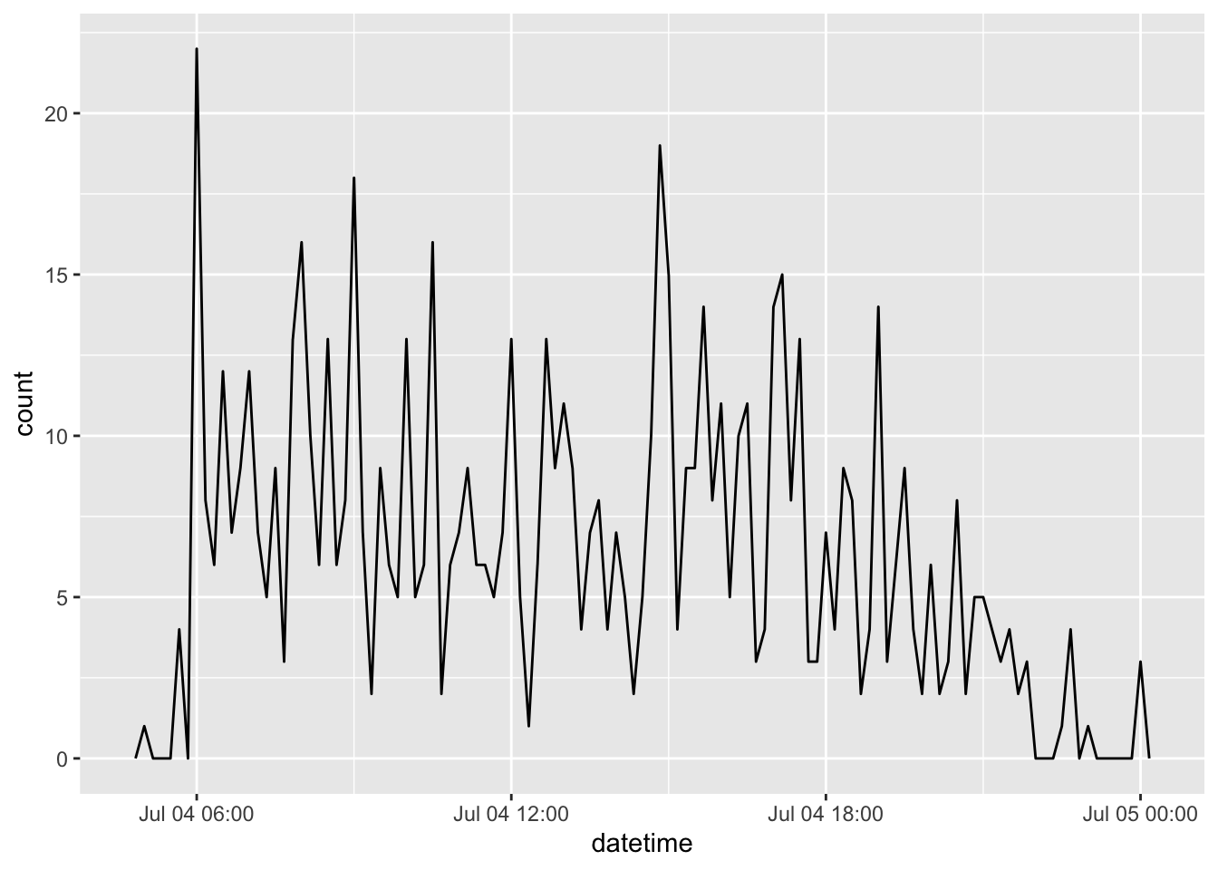
- It also makes it easier to filter by date using
as_date()andymd.

as_datetime()tries to coerce an object to aPOSIXctobject.
3.3.5 Getting/Setting Components of a Date-Time
3.3.5.1 Getting (extracting) the Components of a Date-Time
year()extracts the year.month()extracts the month.week()extracts the week.mday()extracts the day of the month (1, 2, 3, …).wday()extracts the day of the week (Saturday, Sunday, Monday …).yday()extracts the day of the year (1, 2, 3, …).hour()extracts the hour.minute()extract the minute.second()extracts the second.
[1] "1970-01-02 03:51:44 UTC"[1] 1970[1] Jan
12 Levels: Jan < Feb < Mar < Apr < May < Jun < Jul < Aug < Sep < ... < Dec[1] 1[1] 2[1] Fri
Levels: Sun < Mon < Tue < Wed < Thu < Fri < Sat[1] 2[1] 3[1] 51[1] 443.3.5.2 Setting the Components of a Date-Time
- You can use the same functions to set or overwrite components of a date-time.
[1] "1970-01-02 03:51:44 UTC"[1] "1988-01-02 03:51:44 UTC"- Use
round_date()to round to the levels of individual components. - There is also
floor_date()andceiling_date().
3.3.6 Three Different Types of Time Spans
3.3.6.1 Durations - Keeping track of Seconds
- A
durationcounts the exact number of seconds in a time span, between two dates. - Durations allow exact comparisons with other durations.
- However, they don’t always match the number of hours, months, or days you might calculate.
- We can find out Lady Gaga’s “approximate” age using durations.
[1] "1271548800s (~40.29 years)"- Create durations from years with
dyears(), from days withddays(), etc..
[1] "31557600s (~1 years)"[1] "86400s (~1 days)"[1] "3600s (~1 hours)"[1] "60s (~1 minutes)"[1] "1s"- You can add durations to date-times, but it always adds seconds.
- If there is a daylight savings change, you get weird results (add a day but the time is not the same as the time the previous day).
3.3.6.2 Periods
- Periods track the change in the human “clock time” between two date-times by ignoring actual physical time spans.
- Adding a
periodtakes into account daylight savings.
- Adding a
- See help for periods to be aware of the unintuitive calculations that can result if not careful.
3.3.6.3 Intervals
- Intervals record time spans as a sequence of seconds beginning at a specified date.
- Intervals are like durations, but with an associated start time.
- Intervals and durations are good for physical processes that don’t care about human clock time.
- Working with intervals requires some care:
- Divide an interval by a duration to determine its physical length.
- Divide an interval by a period to determine its implied length in clock time.
3.3.7 Time Zones
Time zones are specified using the
tzortzonearguments (for example, in the call toymd_hms()above).- Time zones are specified by “continent/city.” For example,
"America/New_York"and"Europe_Paris". - You can see a complete list of time zones with
OlsonNames(). - You can also use
tz = Sys.timezone()to use the time zone of the computer you are working on.
- Time zones are specified by “continent/city.” For example,
The default time zone is
UTC(which has no daylight savings).- Coordinated Universal Time UTC) is the successor time standard to Greenwich Mean Time (GMT) which is a specific time zone.
You usually don’t have to worry about timezones unless they loaded incorrectly. For example, R might think it’s
UTCeven though it should beAmerica/New_Yorkand then forget daylight savings.If a date-time is labeled with the incorrect time zone, use
force_tz()to change it.
[1] "2014-01-01 10:01:11 UTC"[1] "2014-01-01 10:01:11 EST"[1] "2014-01-01 10:01:11 EST"- If the timezone is correct, but you want to change it, use
with_tz().
3.4 Factors
3.4.1 Introduction
R uses the class factor to represent categorical data, i.e., a variable where each observational/experimental unit belongs to one and only one group, category, or level out of a finite set of groups, categories, or levels.
Being designated as a factor allows R to provide special treatment to the data
- Hair Color could be a factor with levels: Auburn, Red, Brown, Black, Blonde, …
- City sizes: Small, Medium, Large, or Megalopolis
- Major: Data Science, Mathematics, Statistics, or Other
Factors may have words as labels for the levels but they are different from a character variable such as “Brown” or “Small”:
- Factors have a fixed (usually small) number of “levels” (possible values)
- A character variable, e.g., “City_name”, can have many different values.
- Factors have a default ordering of the levels.
- Character variables are only ordered through alpha-numeric sequencing.
- The default ordering for factors in R is alpha-numeric but you can change it to whatever makes sense for the problem.
- Ordering determines how categories are arrayed (ordered) in plots.
3.4.2 Factors have Two Different Representations
When we look at the data, we see the labels of the levels be they words or numbers.
- Use
levels(factor_var)to access the labels and the order of the levels.
R actually stores factors as integers from 1, 2, … number of levels.
- Use
as.numeric(factor_var)to access the stored integer values.
Example: An experimental treatment has levels 2, 15, 32, and 51.
[1] "51" "32" "15" "2" "32"[1] 51 32 15 2 32
Levels: 15 2 32 51[1] "character"[1] "factor"[1] "character"[1] "integer"[1] 51 32 15 2 32[1] 4 3 1 2 3
Note
As of R 4.1.0, combining factors with c() now creates a new factor with changed levels, not a factor with integrated levels.
[1] x1 x2 x3 x4
Levels: x1 x2 x3 x4[1] y1 y2 y3
Levels: y1 y2 y3[1] 1 2 3 4[1] 1 2 3[1] x1 x2 x3 x4 y1 y2 y3
Levels: x1 x2 x3 x4 y1 y2 y3[1] 1 2 3 4 5 6 73.4.3 Creating Factors
3.4.3.1 Both {readr} and Base R have Functions to Create Factors
You can use readr::parse_factor() or base::factor() to create a factor variable.
- However, they sort differently by default.
readr::parse_factor()returns better warnings.
Let’s create a factor for the months of the year using their standard abbreviations.
- Note the differences in the order of the levels
[1] "Jan" "Feb" "Mar" "Apr" "May" "Jun" "Jul" "Aug" "Sep" "Oct" "Nov" "Dec" [1] Jan Feb Mar Apr May Jun Jul Aug Sep Oct Nov Dec
Levels: Apr Aug Dec Feb Jan Jul Jun Mar May Nov Oct Sep [1] Jan Feb Mar Apr May Jun Jul Aug Sep Oct Nov Dec
Levels: Jan Feb Mar Apr May Jun Jul Aug Sep Oct Nov Dec [1] 5 4 8 1 9 7 6 2 12 11 10 3 [1] 1 2 3 4 5 6 7 8 9 10 11 12Both functions assume the levels are the unique values of the vector but they take different approaches to how to “order” the levels
- Base R
factor()sets the order of the levels to be the same order returned bysort(). readr::parse_factor()sets the order of the levels to be the order of the values as introduced in the data.- You can change the order to be alphabetical using the
levels = sort(x)argument
- You can change the order to be alphabetical using the
To access or extract the levels of a factor (and their order) use the levels() function.
[1] "Jan" "Feb" "Mar" "Apr" "May" "Jun" "Jul" "Aug" "Sep" "Oct" "Nov" "Dec" [1] "Apr" "Aug" "Dec" "Feb" "Jan" "Jul" "Jun" "Mar" "May" "Nov" "Oct" "Sep"- You can count the number of levels with
nlevels().
3.4.4 The Tidyverse {forcats} Package
The {forcats} package provides functions to make it easier to manipulate factors.
- All forcats functions begin with
fct_. So you can typefct_then use tab-completion to scroll through the possible functions. - {forcats} is loaded with the {tidyverse} package so there is no need to reload it after loading {tidyverse}.
Three common tasks:
- Change the order of the levels:
fct_reorder(): Reorder the levels of a factor based on the values of another variable.fct_relevel(): Reorder the levels of a factor manually.fct_infreq(): Reorder the levels of a factor by the frequency of its values in the data.
- Change the values of the levels (the labels)
fct_recode(): Change the labels of the levelsfct_collapse(): Collapsing the least/most frequent values of a factor into “other”.
- Add or Drop levels
fct_expand(): Add levelsfct_drop: Drop unused levelsfct_explicit_na(): Assign a level toNAs so you can plot them. Check the help and compare to Base Rfactor()
3.4.4.1 Change the Order of the Levels
You often want to change the order of the levels of a factor to make the data easier for humans to work with or plots easier to interpret.
- You can reorder the levels manually, e.g., to making working with the data easier.
- You can reorder the levels based on the value of another variable, e.g., for better plotting.
- You can change the order by using a {forcats} function inside a
mutate() - You can change the order by using a {forcats} function inside an
aes()call for a plot.
Let’s use the subset of the data from the General Social Survey stored in the gss_cat data set in {forcats}.
Rows: 21,483
Columns: 9
$ year <int> 2000, 2000, 2000, 2000, 2000, 2000, 2000, 2000, 2000, 2000, 20…
$ marital <fct> Never married, Divorced, Widowed, Never married, Divorced, Mar…
$ age <int> 26, 48, 67, 39, 25, 25, 36, 44, 44, 47, 53, 52, 52, 51, 52, 40…
$ race <fct> White, White, White, White, White, White, White, White, White,…
$ rincome <fct> $8000 to 9999, $8000 to 9999, Not applicable, Not applicable, …
$ partyid <fct> "Ind,near rep", "Not str republican", "Independent", "Ind,near…
$ relig <fct> Protestant, Protestant, Protestant, Orthodox-christian, None, …
$ denom <fct> "Southern baptist", "Baptist-dk which", "No denomination", "No…
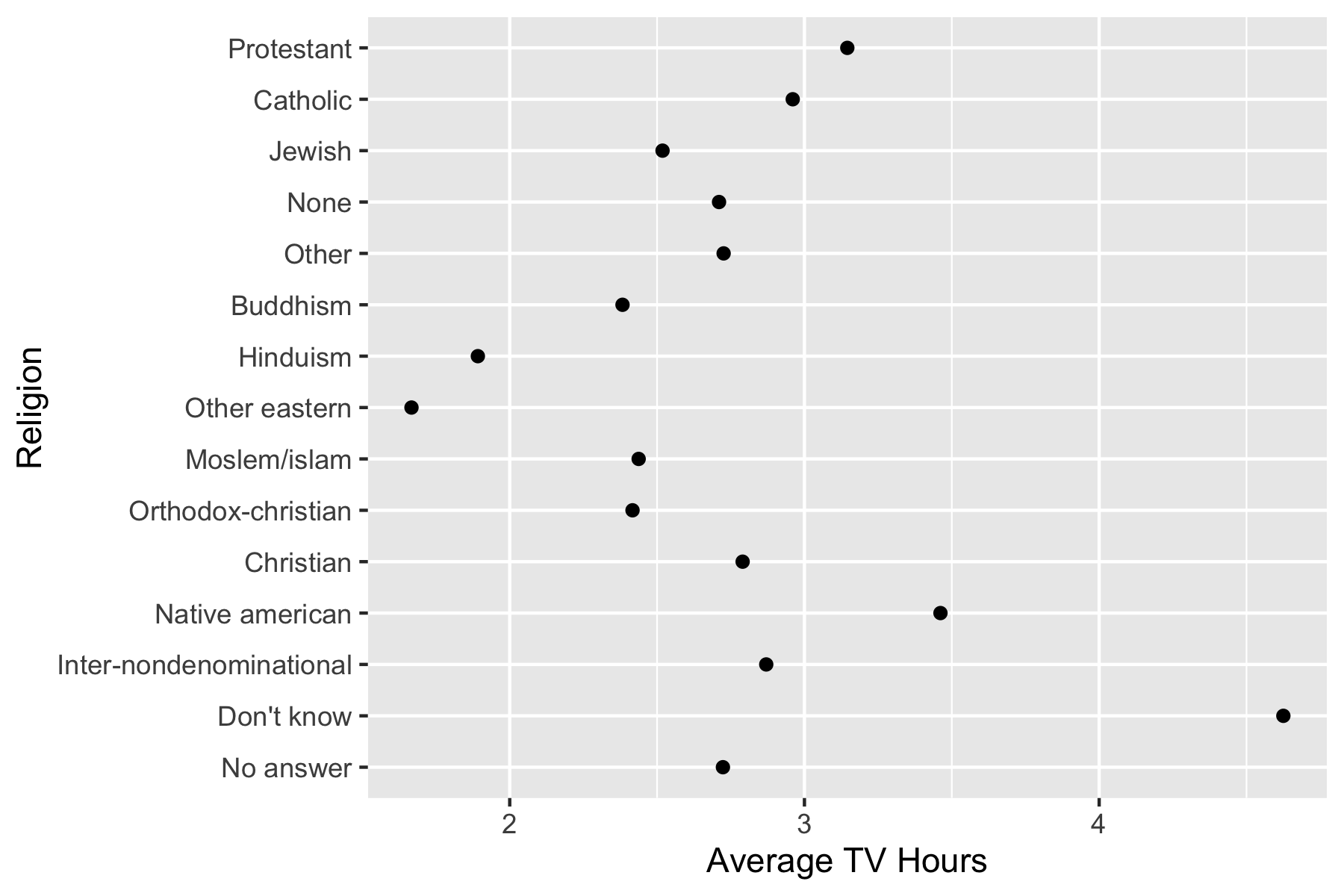
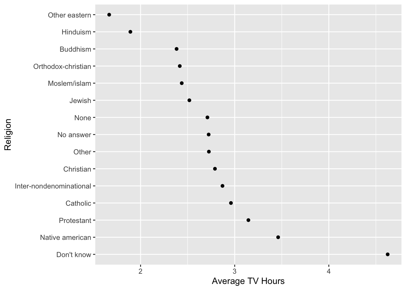
$ tvhours <int> 12, NA, 2, 4, 1, NA, 3, NA, 0, 3, 2, NA, 1, NA, 1, 7, NA, 3, 3…Example: TV hours by Religion - default order.
3.4.4.2 Reordering to be Alphabetical or Based on Order in the Data
If you used factor() or parse_factor() with the default levels you can change the order of the levels.
- Use
fct_relevel()withsortto convert to alpha-numeric order of the levels.
 [1] "Buddhism"                "Catholic"
 [3] "Christian"               "Don't know"
 [5] "Hinduism"                "Inter-nondenominational"
 [7] "Jewish"                  "Moslem/islam"
 [9] "Native american"         "No answer"
[11] "None"                    "Not applicable"
[13] "Orthodox-christian"      "Other"
[15] "Other eastern" "Protestant" - Use
fct_inorder()to convert to the order as in the data.- This will stop with an error if there is a level with no rows in the data!
 [1] "No answer"          "Don't know"         "Other party"
 [4] "Strong republican"  "Not str republican" "Ind,near rep"
 [7] "Independent"        "Ind,near dem"       "Not str democrat"
[10] "Strong democrat" [1] "Ind,near rep" "Not str republican" "Independent"
[4] "Not str democrat" "Strong democrat" "Ind,near dem"
[7] "Strong republican" "Other party" "No answer"
[10] "Don't know" [1] 15[1] 163.4.4.3 Reordering the Levels Based on Another Variable
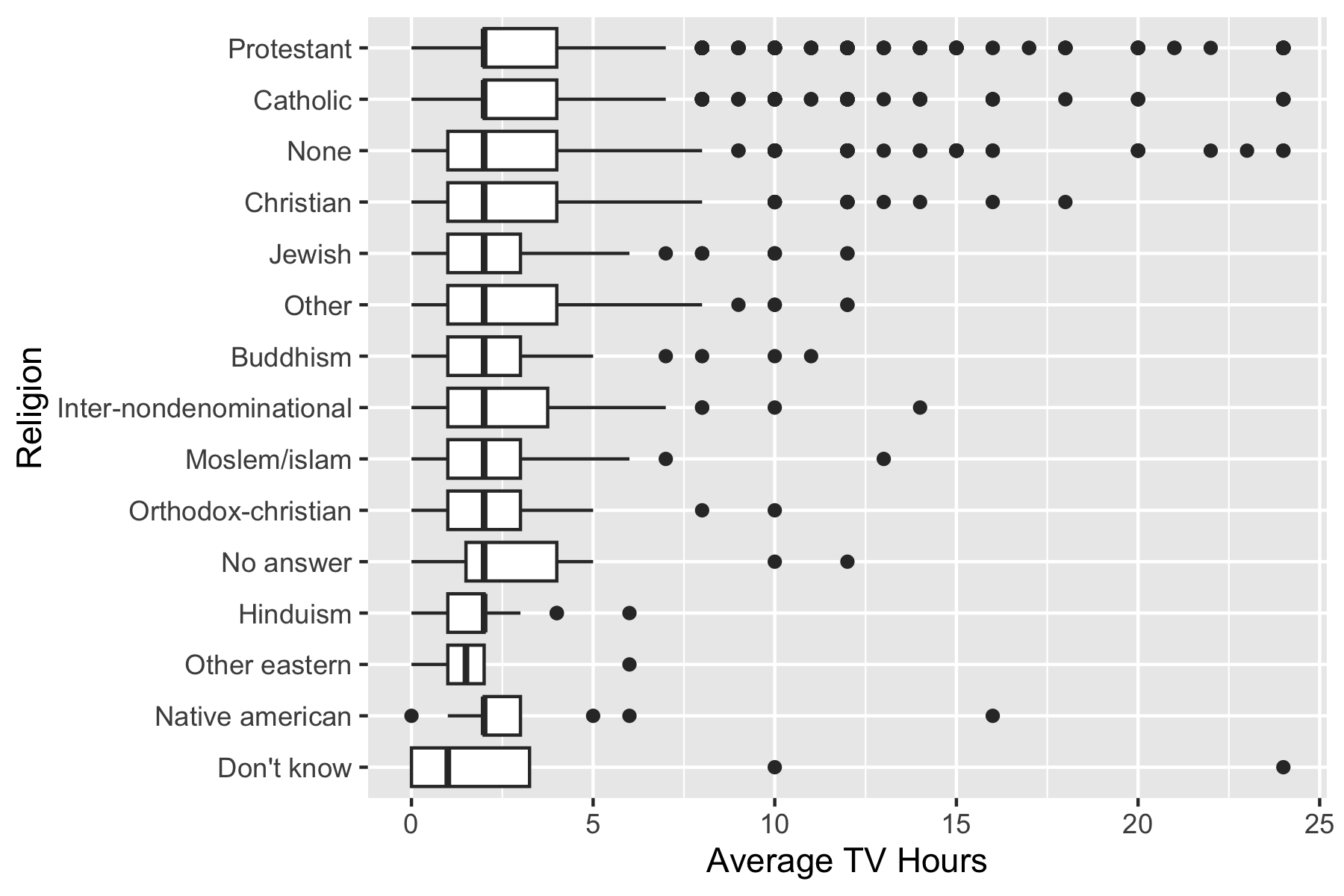
Use fct_reorder(f, x, fun, ..., .desc) to reorder the levels of a factor based on the values of a numeric variable.
.f: The factor vector you want to reorder..x: A numeric vector you want to use to reorder the levels..fun: A function to apply toxwhose result will be used to order the levels off. + default isfun = medianand in ascending orderdesc = FALSE.- Note the
.in the argument names.
- Note the
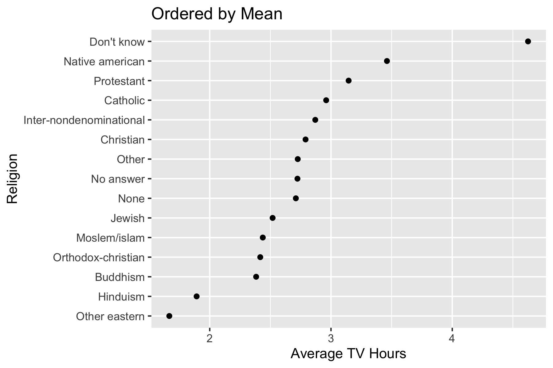
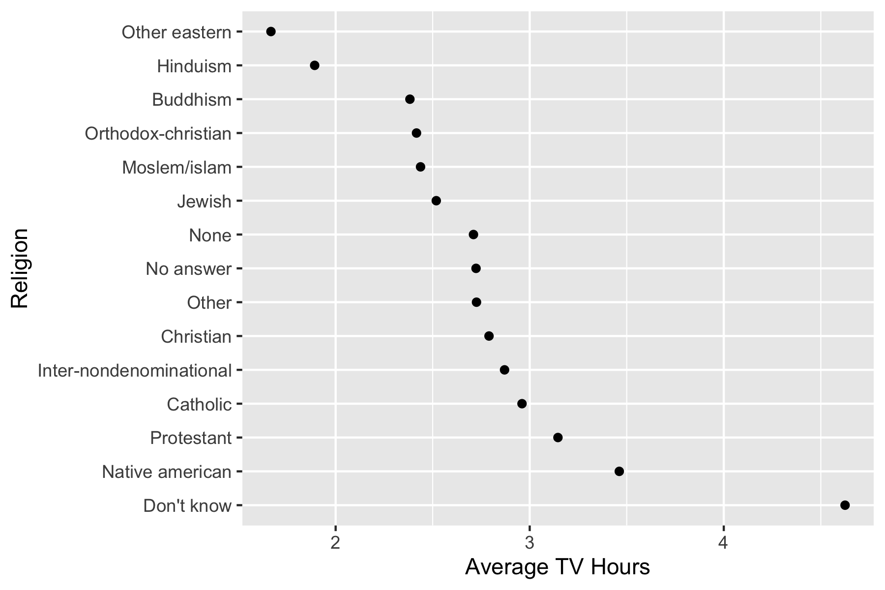
Let’s reorder relig based on the mean of TV hours we calculated earlier.
- We will use
fct_reorder()inside amutate()and save the data frame.
 [1] "No answer"               "Don't know"
 [3] "Inter-nondenominational" "Native american"
 [5] "Christian"               "Orthodox-christian"
 [7] "Moslem/islam"            "Other eastern"
 [9] "Hinduism"                "Buddhism"
[11] "Other"                   "None"
[13] "Jewish"                  "Catholic"
[15] "Protestant" "Not applicable" [1] "Other eastern" "Hinduism"
[3] "Buddhism" "Orthodox-christian"
[5] "Moslem/islam" "Jewish"
[7] "None" "No answer"
[9] "Other" "Christian"
[11] "Inter-nondenominational" "Catholic"
[13] "Protestant" "Native american"
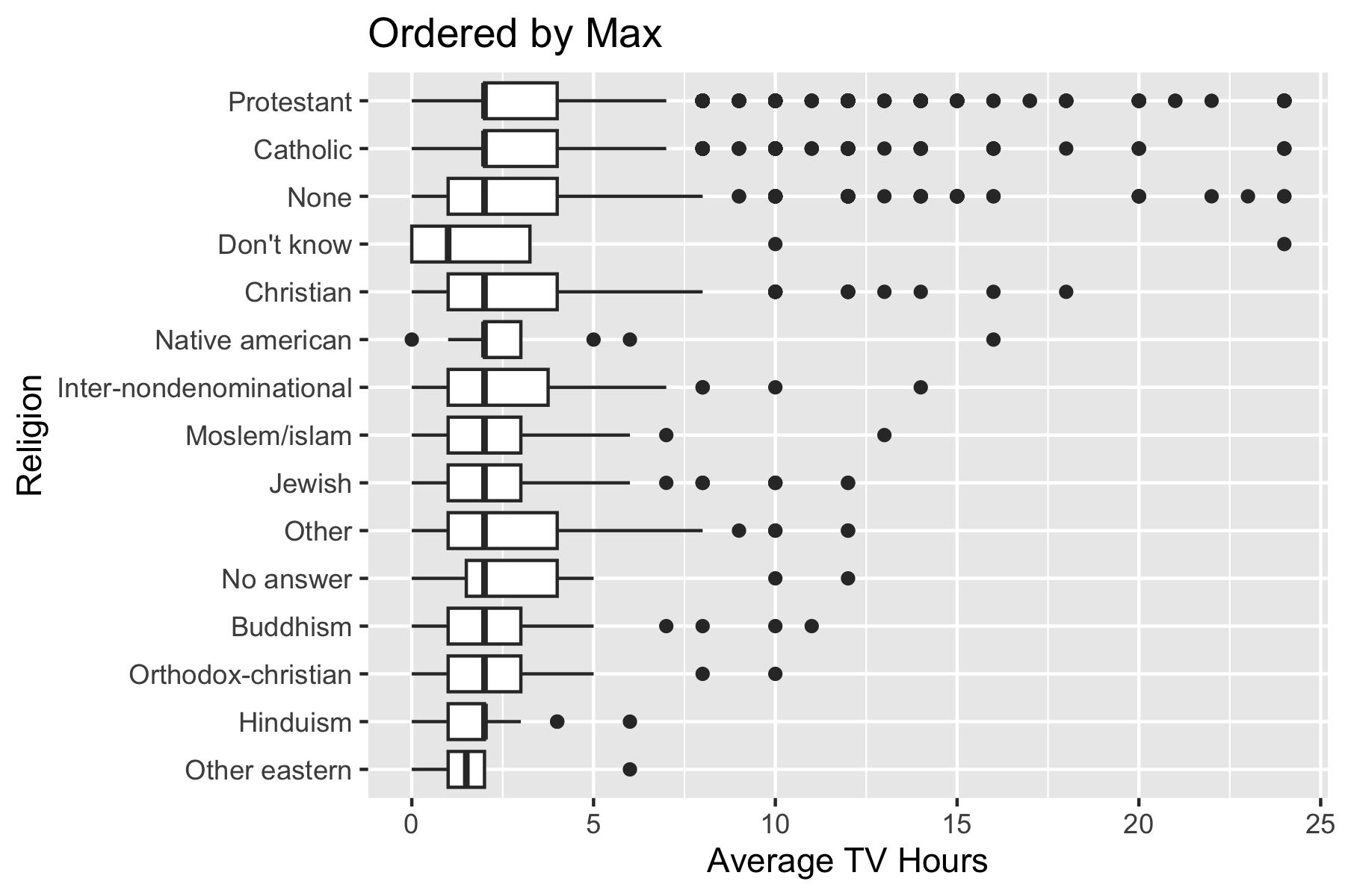
[15] "Don't know" "Not applicable" - Using the
.fun = maxon the original data.
 [1] "No answer"               "Don't know"
 [3] "Inter-nondenominational" "Native american"
 [5] "Christian"               "Orthodox-christian"
 [7] "Moslem/islam"            "Other eastern"
 [9] "Hinduism"                "Buddhism"
[11] "Other"                   "None"
[13] "Jewish"                  "Catholic"
[15] "Protestant" "Not applicable" [1] "Other eastern" "Hinduism"
[3] "Orthodox-christian" "Buddhism"
[5] "No answer" "Other"
[7] "Jewish" "Moslem/islam"
[9] "Inter-nondenominational" "Native american"
[11] "Christian" "Don't know"
[13] "None" "Catholic"
[15] "Protestant" "Not applicable" - The plot now reorders the y-axis according to the new level order.
fct_relevel(.f, ..., after = 0L) also allows you to manually move existing levels to any location you choose.
- Note the use of integer values, e.g.,
2L. - Any levels not mentioned will be left in existing order.
 [1] "None"                    "Other eastern"
 [3] "Hinduism"                "Buddhism"
 [5] "Orthodox-christian"      "Moslem/islam"
 [7] "Jewish"                  "No answer"
 [9] "Other"                   "Christian"
[11] "Inter-nondenominational" "Catholic"
[13] "Protestant"              "Native american"
[15] "Don't know" "Not applicable" [1] "Other eastern" "Hinduism"
[3] "None" "Buddhism"
[5] "Orthodox-christian" "Moslem/islam"
[7] "Jewish" "No answer"
[9] "Other" "Christian"
[11] "Inter-nondenominational" "Catholic"
[13] "Protestant" "Native american"
[15] "Don't know" "Not applicable" [1] "Other eastern" "Hinduism"
[3] "Buddhism" "Orthodox-christian"
[5] "Moslem/islam" "Jewish"
[7] "No answer" "Other"
[9] "Christian" "Inter-nondenominational"
[11] "Catholic" "Protestant"
[13] "Native american" "Don't know"
[15] "Not applicable" "None" [1] No answer Don't know Inter-nondenominational
[4] Native american Christian Orthodox-christian
[7] Moslem/islam Other eastern Hinduism
[10] Buddhism Other None
[13] Jewish Catholic Protestant
16 Levels: Other eastern Hinduism Buddhism Orthodox-christian ... Not applicablefct_infreq() reorders the levels by frequency of a level in the data from largest to smallest.
fct_count(): will count the number of values in each level
 [1] "Protestant"              "Catholic"
 [3] "None"                    "Christian"
 [5] "Jewish"                  "Other"
 [7] "Buddhism"                "Inter-nondenominational"
 [9] "Moslem/islam"            "Orthodox-christian"
[11] "No answer"               "Hinduism"
[13] "Other eastern"           "Native american"
[15] "Don't know" "Not applicable" # A tibble: 16 × 2
f n
<fct> <int>
1 Protestant 10846
2 Catholic 5124
3 None 3523
4 Christian 689
5 Jewish 388
6 Other 224
7 Buddhism 147
8 Inter-nondenominational 109
9 Moslem/islam 104
10 Orthodox-christian 95
11 No answer 93
12 Hinduism 71
13 Other eastern 32
14 Native american 23
15 Don't know 15
16 Not applicable 0fct_rev() reverses the order of the factors.
3.4.4.4 Change Orders of Levels in a Plot
Instead of mutating the data before the plot, you can change the levels inside the aes() call.
3.4.5 Change the Values of the Levels (the Labels)
Use fct_recode() to manually change the labels for the levels.
- The new label level goes on the left of the equals sign.
- The old label level goes on the right.
- Think
New <- Oldjust likemutate().
gss_cat |>
  mutate(partyid = fct_recode(partyid,
                      "Republican, strong"    = "Strong republican",
                      "Republican, weak"      = "Not str republican",
                      "Independent, near rep" = "Ind,near rep",
                      "Independent, near dem" = "Ind,near dem",
                      "Democrat, weak"        = "Not str democrat",
                      "Democrat, strong"      = "Strong democrat"
                      )) ->
gss_cat2
levels(gss_cat2$partyid)
[1] "No answer" "Don't know" "Other party"
[4] "Republican, strong" "Republican, weak" "Independent, near rep"
[7] "Independent" "Independent, near dem" "Democrat, weak"
[10] "Democrat, strong" fct_collapse(): combines multiple levels into one level.
# A tibble: 10 × 2
   f                      n
   <fct>              <int>
 1 No answer            154
 2 Don't know             1
 3 Other party          393
 4 Strong republican   2314
 5 Not str republican  3032
 6 Ind,near rep        1791
 7 Independent         4119
 8 Ind,near dem        2499
 9 Not str democrat    3690
10 Strong democrat     3490
gss_cat |>
mutate(partyid = fct_collapse(partyid,
missing = c("No answer", "Don't know"),
other = "Other party",
rep = c("Strong republican", "Not str republican"),
ind = c("Ind,near rep", "Independent", "Ind,near dem"),
dem = c("Not str democrat", "Strong democrat")
)) ->
gss_cat2
fct_count(gss_cat2$partyid)# A tibble: 5 × 2
f n
<fct> <int>
1 missing 155
2 other 393
3 rep 5346
4 ind 8409
5 dem 71803.4.6 Add or Drop Levels
fct_expand(): adds one or more new levels.
[1] A B
Levels: A B[1] A B
Levels: A B C Zfct_drop(): removes any levels that are unused.
[1] A B
Levels: A B C[1] A B
Levels: A BExample of using fct_drop to clean up gss_cat$relig so we can use fct_inorder.
 [1] "Protestant"              "Orthodox-christian"
 [3] "None"                    "Christian"
 [5] "Jewish"                  "Catholic"
 [7] "Other"                   "Inter-nondenominational"
 [9] "Hinduism"                "Native american"
[11] "No answer"               "Buddhism"
[13] "Moslem/islam"            "Other eastern"
[15] "Don't know"
fct_explicit_na() allows you to create a level for NAs in case you want to plot them as a category.
3.5 Tidyverse Review
3.5.1 Things to Consider with {readr}
- Use it!
- Always use a relative path instead of an absolute path to ensure reproducibility.
- You can use the syntax with the appropriate sequence of
,and/to navigate or the {here} package.
- You can use the syntax with the appropriate sequence of
- Use the
read_csv()function instead of theread.csv()function for better warnings and speed. - Use the
na =and otherread_csv()arguments to reduce parsing errors.
3.5.2 Things to Consider with {ggplot2}
- Using a log scale is not the same as logging the data.
- Both give a different view of the data but the log scale preserves the values and changes the “scale” on the axis.
- Logging the data changes the values of the data and the values of the scale.
- You may have to use log scale on the plot and then log the data in the statistical model.
- Whenever you are asked to plot data for an association between two variables, consider the question in terms of how does the variable on the X axis explain what is happening on the Y axis (the response). Typically read the problem as plot Y vs X.
- Whenever plotting to look for an association, use a smoother.
- Start with the default, non-linear,
geom_smooth(se = FALSE). - Set
method = "lm"to see a linear smoother. - On assignments, check the question or rubric if in doubt which to use.
- Start with the default, non-linear,
- Consider the difference between a linear smoother (Ordinary Least Squares (OLS) regression line) and the default
geom_abline()wherey = x.- The first is useful for examining if there is a linear relationship between two variables.
- The second is useful for determining if there is a pattern to the relative values of the two variables compared to the
y = xline.
- Consider the options for
ggtitle()andlabs(). - Consider using
str_glue()orglue()to create dynamic labels. - Use themes to change colors, legends, and adjust other elements of the plots
- Consider
ggthemes::scale_color_blindor alternative color palates such as the viridis family for accessibility. - Remember the difference between
colorandfillfor different kinds of plots.
3.5.3 Things to Consider with {dplyr}
- Avoid using a
full_join()as it can lead to trouble. Consider aleft_join()instead. - Consider the filtering joins:
anti_join()andsemi_join()as they save a lot of code. - If you did not cover
across()with helper functions in your previous class review Column-wise operations vignette. - If you did not cover
rowwisein your previous class, review Row-wise operations vignette. - An instruction like “for each xxx”, suggests the need to use
group_by()for one or more variables.- If the statement says : for each “xxx, yyy, and zzz” then consider grouping by the three things.
- Think about whether you want to
summarize()ormutate()and the implications of one over the other.summarize()reduces rows and columns (only those in the summarize and the grouping variables).mutate()keeps all the rows and columns but makes duplicate values.
- Consider how to deal with the output of using
group_by(), especially after grouping more than one variable and then usingsummarize(). Do you want toungroup()or do you want to operate next on a grouped data frame? - Consider how the
slice()functions work with ties as compared tohead().- If a problem says find the
nlargest values, that generally suggests usingslice_max( order_by = xxx, n = n)and not usingarrange()and thenhead(n = n)in case there are ties.
- If a problem says find the
3.5.4 Things to Consider with {tidyr}
- You can reshape the data to get the variables you need to do some calculations and then reshape again.
- Use the
pivot_wider()andpivot_longer()functions and not the deprecatedgather()andspread(). - Use the additional arguments for the pivots to minimize extra code to transform the values/class of the variables or reduce
NAs.
3.6 Strategies for the Course and Data Science
3.6.1 Data Science Cheat Sheet
There are many cheat sheets for tidyverse and other R packages. Here is one for doing well on assignments (and future data science work).
- Use the starter file. If you don’t, you run the risk of missing a part of a question and your homework is harder to grade. Be sure to rename the file and put your name as Author.
- Read the Problem all the way to the end.
- Are there multiple parts?
- What is the output required to answer the question?
- What format should the answer be in?
- Are there restrictions on the packages to be used?
- Does it require re-saving the modified data? If so to what/where?
- Check the Rubric in the HTML file to see if it makes sense.
- Organize the files in the proper directories
- Look at the data after loading.
- Visually inspect the data after you read it in.
- Check for parsing errors - if so - why?
- Check the number of rows and columns - does it make sense?
- Is the data in the right shape?
- Does it have the right variables?
- Develop a Strategy and Plan for how to Solve the Problem
- Think about the starting point and where you want to end up.
- Some problems may be easier by thinking from the end state and working backwards towards the beginning.
- What should the final data frame look like and how do I get there.
- What should it look like on the way?
- How can I test I am getting the right results along the way?
- Build a little - Test a little!
- Do not try to solve all the problem at once!
- Enter a few lines and check your results.
- Does the data have the right shape?
- Does it have about the right number of rows/columns?
- Are the values reasonable?
- Is there another source you can check to validate your results?
- Use the Help function, RStudio Cheat Sheets, Google, StackOverflow etc..
- You are not expected to remember every bit of syntax or possible argument to a function.
- You are expected to be able to read the help.
- If a problem says use function or an argument to do something, use the help to get to the function or argument and how to use it.
- The arguments are there to save you extra lines of code and computation to make your code faster and easier to read.
- Save and Commit Early and Often!
- Push Regularly
- When creating plots, check the instructions/rubric for any specifications or constraints.
- Read the HTML file if you are trying to reproduce a plot.
- When interpreting a plot - don’t just describe it, but say what you think it means and what the implications for your analysis might be.
- Render to HTML and then add, commit, and push and then submit a note on Canvas.
3.6.2 Things to Avoid
- Do Not Use Absolute Paths. If your name is in the path it means the repo is not reproducible on someone else’s machine. Use Relative Paths.
- Do Not Show Excessive Data.
- We will be using data sets that can easily generate hundreds of pages in your HTML output.
- That is not a good thing.
- Depending upon the structure of the data use
head()orglimpse()if you want to check something. - You can also use the code chunk option
include: FALSEso no results from the chunk go into the output.
- Do Not Submit Messy Code.
- Do follow tidyverse style and especially do the following:
- Use a linebreak after each pipe.
- Use a linebreak after each + in ggplot2.
- Use a linebreak after each
{and}.
- Put spaces on both sides of infix operators, e.g.,
=and+,<-,->,%>%or|>.
- Put spaces on both sides of infix operators, e.g.,
- Use the {lintr} or {stylr} packages (and RStudio Addins) to assist.
- Tidyverse style is not just about looking pretty but being able to read and debug code faster than if the code is messy.
- Do follow tidyverse style and especially do the following:
- Do not use unusual packages for most assignments.
- Some assignments and the group project may require specialized packages not taught in class. For the most part however, any packages you need will be covered in class.
- Do not use excessive Base R when a tidyverse function is appropriate.
- This is a course focused on tidyverse approaches so there is no need to use
grep,lapply, etc.. - Base R primitives and common functions without tidyverse equivalents are fine.
- This is a course focused on tidyverse approaches so there is no need to use
- Do not set or change the working directory in an .Rmd file.
- The default is the directory where it is stored.
- Use relative paths to load data or save output as desired.
- Do not leave lots of excess code in an .qmd file.
- It’s great to try things out but no one wants to see all extra code.
- Delete it or comment it out (use CTRL Shift C or Command Shift C).
- Even when submitting code that is not working, only include what you think is the “closest” to what you are trying to do.
3.6.3 Final Thoughts
Use the RStudio capabilities to assist you. Use the environment, files, and packages panes to keep track of what is going on.
Use RStudio Projects to simplify working with Git and GitHub and consider the Git Pane for efficient routine workflow.
Experiment with small examples. If you are not sure what the code is doing, use the .Rmd or console to try on a small data set such as mtcars that is already present.
Collaborate with your peers on what the question means and what the answers should look like. Do not share code or show code to each other.
Ask the TA or instructor for help and /or office hours! Push your code to GitHub so the instructor can see it as screen shots are always missing some context.
3.7 Using Quarto for Literate Programming
Quarto is a new open-source scientific and technical publishing system from Posit.
Quarto users can:
- Create multi-language projects with R, Python, Julia, Observable, … (R not required).
- Use one document to create reports, journal articles, presentations, web content,… in HTML, PDF, Word, PowerPoint, … All Formats.
- Write/code in multiple tools such as RStudio, JupyterLab, VS Code, Text Editors, ….
- Use .Rmd files or python .ipynb, or “upgrade” to .qmd for more features ….
- Collaborate across teams using different formats, languages, and tools.
Quarto has a shallow learning curve, especially for R Markdown users.
- It’s the next-generation of R Markdown and Posit’s focus for new capabilities.
- Comes “batteries included” so no need to manage multiple packages.
- Extensive on-line documentation, an active community, and numerous videos and blogs, e.g. A Quarto tip a day .
- Multiple themes with options for customized CSS/SCSS, or \(\LaTeX\).
3.7.1 Quarto Unifies the R Markdown Ecosystem
Quarto incorporates capabilities of multiple packages to allow for diverse outputs:
- Documents: HTML, PDF, Word
- Websites
- Blogs
- Web-Books
- Presentations:
- HTML (Revealjs)
- PDF (Beamer)
- PowerPoint (.pptx)
Quarto supports multiple languages: R, Python, Julia, Observable, ….
- Can use either Knitr or Jupyter computation engines (R is NOT required).
- Can support R and Python in the same file with R {reticulate} package.
Quarto operates as a Command Line Interface in the Terminal window and ….
- Is integrated into RStudio (v2022.07+) and works in JupyterLab , VS Code, Text Editors.
- Can render python .ipynb.
Quarto supports \(\LaTeX\) and math with MathJax (including AMSmath).
3.7.2 Quarto Extends R Markdown
Quarto creates plain-text files using YAML and R Markdown tags.
- If you are new to RStudio or R Markdown see RStudio Hello, Quarto Tutorial or Authoring: R Markdown Basics.
- Additional tutorials and sections under Authoring describe many new features of Quarto.
Quarto works with .Rmd files but recommends upgrading for more features.
- Quarto files end in
.qmdinstead of.Rmd. - Use a slightly different YAML Syntax to make it easier to change outputs and be consistent across languages and tools.
format: htmlinstead ofoutput: html_document.
- Use
#| option: valuefor chunk options instead of fitting into the chunk header. - You can edit to convert the chunk options or use
knitr::convert_chunk_header().knitr::convert_chunk_header("your.Rmd", "your.qmd", type = "yaml")
3.7.3 Getting Started
Getting Started with Quarto in RStudio is a good resource if you are new to RMarkdown.
Quarto is fully integrated into RStudio (V2022.07 +).
- You can operate using the IDE or use the console command line.
You can use the IDE to:
- Create new Quarto documents using the menu for
File/New File/Quarto Document. - Auto-complete yaml and chunk options.
- Open an existing
.Rmdfile or edit an existing.qmdfile as usual.
You can add many options to your YAML and see the auto complete in action.
---
title: "Untitled"
format: html
editor: visual
date: today
theme: cerulean  # lots of options for themes
number-sections: true # automated numbering of headings
self-contained: true # For HTML to allow sharing of complete files (makes them larger)
code-fold: true # collapse code chunks with option to show the code
execute:        # set global code chunk options as in Rmarkdown Setup chunk
  echo: true
  eval: true
  freeze: true  # New capability to save calculations to speed later renders
---
3.7.3.1 Quarto has an Expanded Visual Editor in RStudio
The RStudio Visual Editor provides a WYSIWYM capability.
- It shows what you “mean” but does not completely render all the elements on the page.
- You can preview the rendered version in either the Viewer or Presentations Panes or switch to a Window view in a browser using the open browser icon
 .
.
The Visual Editor provides access to many formatting options and special features through the Format and Insert menus.
I often go back and forth between the Visual Editor and the Source Editor as I find it much easier to “fix” things in the Source Editor (except for tables).
The Visual Editor is great for inserting features such as tab panels, columns, callout blocks, or span formatting and then going to the Source Editor to fine tune them.
Tables are still limited in R Markdown but the Visual Editor makes it much easier to create and edit large tables.
WarningThe Visual Editor will “Escape” errors with a \\.
If you edit something in source editor, such as a table or math, and there is an error in it and you try to see it in the visual editor, Quarto will “escape” all special characters such as [ or | with a \ so you have a lot to clean up manually. Using the IDE ![]() Find and Replace can help.
Find and Replace can help.
3.7.4 Writing Math and \(\LaTeX\) in Quarto
Quarto supports \(\LaTeX\) for writing math equations (\(\text{Area} = \pi r^2\)), matrices, as well as numbering and cross-references using {#eq-my-equation}.
\[ \begin{align} \hat{\beta}_1 & = \frac{\sum(x_i - \bar{x})(y_i - \bar{y})}{\sum(x_i - \bar{x})^2} \\ \hat{\beta}_0 & = \bar{y} - \hat{\beta}_1x \end{align} \tag{3.1}\]
\[ A = \begin{bmatrix}a_{11}&a_{12}&\cdots &a_{1m} \\ \vdots & \vdots & \ddots & \vdots\\a_{n1}&a_{n2}&\cdots &a_{nm}\end{bmatrix} \]
\[ m_{ij} = (a_{i1}b_{1j} + a_{i2}b_{2j} + \cdots + a_{im}b_{mj}) = \sum_{k=1}^{m} a_{ik}b_{kj} \tag{3.2}\]
3.7.5 Divs and Spans
Quarto allows you to create a Div or a Span to customize sections of the document, or pieces of code.
See Divs and Spans for detailed help.
A Div creates a block (division) of the document that gets special treatment.
- Divs are used for many built-in features to include tab-sets and callout boxes.
- You can customize a Div and nest Divs within other divs.
- Use the Visual editor to Insert and or enter a pair of
:::to delineate the div. - The Div should be separated by blank lines from preceding and following blocks.
A Span is used for giving special treatment to a section (span) of text.
- You can customize a Span using CSS and nest Spans within other Spans
- Use the Visual editor to Format a span or delineate the text inside and add the attributes you want after it using
[This is *some text*]{.class key="val"}.
I often use the Visual editor to insert a div or span, especially tabsets or callout boxes, and then switch to the Source editor to move content around.
3.7.6 Quarto Extensions
Quarto has an array of Extensions that allow you to add additional capabilities to your document.
- Extensions exist for Shortcodes/Filters, Journal Articles, Custom Formats, and Revealjs.
Extensions must be installed for each Quarto project.
Consider the FontAwesome extension for including 2,000 free icons in either HTML or PDF.
Install using the terminal with
quarto install extension quarto-ext/fontawesome.This will create a directory
_extensions/quarto-ext/fontawesomeUsers can adjust the size, color, and accessible text for the icons. {}
Use shortcode {{< fa name >}} : fa thumbs-up fa folder fa chess-pawn fa brands bluetooth fa brands github size=2x fa battery-half size=Huge fa envelope title= “an envelope”
See Icons in Quarto for more ideas.
3.7.7 Scholarly Writing
Quarto has features to simplify formatting for publication on the web or in academic journals.
Cross References provide numbered references and hyperlinks to elements of your document that you choose.
Labels {#type-name} go after the element (separated by a space) or as an option in a code chunk, e.g., #| label: fig-plots
- Common elements include Figures
#fig-, Tables#tbl-, equations#eq-, Section Headings#sec-, and others - The
namemust be unique within the document (or across documents in a project) - Add
crossref: chapters : trueto the YAML to indicate that top-level headings (H1) in your document correspond to chapters, and cross-references should be sub-numbered by chapter.
Figures and tables, whether generated by markdown or in a code chunk, must have a Caption as well to be cross-referenced.
To reference a labeled item, use @type-name for the item of interest.
Quarto can support BibLaTeX (‘.bib’) or BibTeX (‘.bibtex’) files for Citations
- Add the relative path to the file to the YAML, e.g.,
bibliography: references.bib - Recommend using Zotero with the Better Bibtex addin to manage your collection of citations.
Quarto uses the standard format [@citation-key where citations go inside square brackets and are separated by semicolons - The citation-key must be present in the referenced .bib file.
The default is the Chicago Manual of Style author-date format, but you can specify a custom format by adding csl: myformat.csl to the YAML where myformat is a file such as found at Zotero Style Repository
Quarto has Templates for several journals and Posit and the open source community are building more (and you can build your own as well).
For pre-built templates, use the terminal to install the extension, e.g., quarto install extension quarto-journals/jasa.
Then edit the YAML to use the template format, e.g., format: jasa-pdf.
The pre-built templates usually have an example .qmd file with their options.
3.7.8 Customizing Quarto
Quarto has many options to customize your output for each type of format.
- The quarto Gallery has lots of examples.
If one of the built in themes fonts, colors, sizes, layout does not suit your purpose, you can create your own variations.
- for HTML: embed HTML tags or more generally, use a custom SCSS file to adjust existing CSS classes or add your own.
- for PDF, you can use any option Pandoc allows for PDF Latex.
You can change the page layout
- Add columns using a div
- Move content to the margins
You can choose different languages for the document.
3.7.9 Quarto Projects
3.7.9.1 Quarto Projects Overview
Quarto Projects are not the same as RStudio Projects.
A Quarto Project is a folder with (usually) multiple documents that should be rendered together under common options.
- You can still override the common options though for portions of the project
Projects are used to create articles from multiple source documents, websites, books or other collaborative efforts.
Quarto projects are characterized by their use of a _quarto.yml file which serves as a configuration file for the project.
- Edit the
_quarto.ymlfile to define the elements of the project and any common options you want to apply across the project. - Adding the The YAML
freeze: autooption will keep track of all documents that have been rendered and only re-render a file when it has changed.
Use the RStudio File/New project command or run quarto create_project in the terminal in the directory where you want to create a project.
3.7.9.2 Personal Websites and Blogs
The {blogdown} package is an R Markdown based package for creating personal websites or blogs using Hugo.
Quarto streamlines creating a website/blog with many options for customizing and enhancing it over time.
The Quarto Guide Creating a Website shows how to create a website or a blog.
- These are both Quarto Projects as you use multiple .qmd files for a website or blog.
- A Website organizes your files based on the structure navigation you define in the _quarto.yaml , e.g. navigation bars of Tabs and/or Menus and/or a sidebar menu etc..
- A Blog uses a listing page which will search for files under a directory and organize the files by date/time.
If you want a combination of website and blog, recommend creating a website and then in the navigation add a .qmd file with the line listing: default in the YAML header.
Quarto generates a standard structure of HTML files for all the contents of your website/blog.
Thus you can publish it in a wide variety of places for free.
Quarto has its own site, quarto.pub.com, where you can publish your work.
Once you set up an account, it is a two step process:
- Render your website in RStudio (this is where the
freeze: autospeeds things up). - Publish your website using the command
quarto publishin the terminal window in the project directory.
You can add new files and update your website as often as you wish.
    project:
      type: website
    website:
      title: "Richard Ressler's Data Science Site"
      navbar:
        left:
          - text: "Home"
            file: index.qmd
          - text: "Data Sets"
            file: data_sets/data_sets.qmd
          - text: "Blog"
            file: posts/posts.qmd
          - text: "Talks"
            file: talks/talks.qmd
    execute:
      freeze: false # re-render only when source changes
    format:
      html:
        theme:
          light: flatly
          dark: darkly
        css: styles.css
        toc: true
    editor: visual
3.7.10 Quarto Summary
Quarto is the next generation of R Markdown and integrates capabilities from multiple packages for a more consistent approach to literate programming and scientific and technical publishing.
These notes just scratch the surface of its capabilities right out of the box and how you can customize your work.
More developments are coming:
- Add Track Changes/Comments in the visual editor for collaboration.
- Add HTML widgets.
- Add more templates for journals.
Use Quarto for reproducible work at AU and beyond!
- The online tutorials and documentation are great places to start!
- See Awesome Quarto for a curated list of resources.
- Try it out! Experiment! Review the Quarto Discussions or Ask a Question.
- Create your Website or Blog and let everyone know what you are up to!