7 Getting Data by Web Scraping
rvest, xml, chromote, rselenium
7.1 Introduction
7.1.1 Learning Outcomes
- Check the Terms of Service and robots.txt prior to scraping.
- Employ Cascading Style Sheet (CSS) selectors in web scraping.
- Use the {rvest} package for web scraping static sites.
- Apply techniques to tidy data after web scraping.
7.1.2 References:
- R for Data Science 2nd Edition Chapter 25 Web Scraping Wickham, Cetinkaya-Rundel, et al. (2023)
- Intro to robots.txt Google (2023)
- {polite} package Perepolkin (2023)
- {rvest} package Wickham (2022)
- {xml2} package Wickham, Hester, et al. (2023)
- {chromote} Chang and Schloerke (2024)
- SelectorGadget for Chrome Cantino (2013)
- SelectorGadget vignette Wickham (2023)
- {readxl} package Wickham and Bryan (2023)
- {googlesheets4} package Bryan (2023)
- {selenider} package Ashby Thorpe (2025)
- {rplaywright} package Siregar (2024)
- {promises} package Cheng (2025a)
- {promises} vignetteCheng (2025b)
- {RSelenium} package Harrison (2023a)
- {RSelenium} vignette Harrison (2023b)
- {httpuv} package Joe Cheng et al. (2025)
- {PDF} Data Extractor package Stricker (2023)
- {tabulapdf} package Sepulveda (2024a)
- {tabulapdf} vingette Sepulveda (2024b)
7.1.2.1 Other References
- W3 Schools HTML Tutorial Schools (2023b)
- W3 Schools CSS Tutorial Schools (2023a)
- W3 Schools Javascript Promises Schools (n.d.)
- Document Object Model Docs (2023)
- Playwright Microsoft (n.d.)
- RSelenium Tutorial Atuo (2025)
- The Ultimate CSS Selector Cheat Sheet scrape-it.cloud (2022)
7.2 Web Scraping
Web scraping is a way to extract data from web sites that do not have APIs, or whose APIs do not provide access to the data you need.
A decade ago, web scraping was fairly straightforward.
However, more modern websites create challenges for scraping as they employ “behind-the-page” techniques to optimize speed while balancing openness (so they can be found and useful) with protecting their intellectual property.
- Building a successful web-scraping strategy starts with a key realization:
What you see in a browser is not (necessarily) what your code gets.
The web page you see as a human using a browser may differ substantially from the content returned to your code when it makes a request to the same URL.
- Many pages (especially older ones) are mostly static HTML, where the content of interest is always present directly in the page source.
- Newer web pages, particularly those optimized for performance and interactivity, rely on one or more techniques that dynamically add content only as required.
- Some pages are “rendered” or “hydrated” after the initial load, with content inserted by JavaScript.
- Some pages deliver only partial content initially and load additional content as the user scrolls (“infinite scrolling”).
- Some pages return different content depending on request headers (especially the User-Agent) or cookies related to consent, location, or experiments.
- Many web sites now actively balance being discoverable (so search engines can index their content) with protecting their intellectual capital.
- As a result, sites may selectively limit, reshape, or obscure the data returned to automated clients, while still presenting full content to human users and allowed search engine crawlers.
- Modern web sites also frequently re-implement and refactor their code, and often there is no visible change to the rendered page.
- Front-end frameworks, build pipelines, and A/B testing can change the underlying structure, class names, or data layout while the page looks identical to a human user.
- Scraping code that relies too closely on a specific page structure may fail without warning and without any change in the URL or visible content.
Taken together, these realities mean successful web scraping is less about finding a clever content selector and more about choosing a strategy that is robust to partial content, dynamic content, client-dependent responses, and structural change.
7.3 Web Scraping and Responsible Data Science - To Scrape or Not to Scrape, that is the question
Is web scraping legal? Yes, but …
- Web Scraping - Legal or Illegal?
- Recent Court cases have ruled in favor of the web scrapers in some circumstances.
- In 2024, a U.S. District Court in the Northern District of California dismissed contract/tort claims that sought to bar scraping of publicly available data, holding those claims were preempted by the Copyright Act. This decision has implications for whether website terms of use can limit scraping for commercial purposes or AI training. Recent District Court decision casts doubt on terms of use barring data scraping
- In an ongoing 2025 Canadian case, news organizations sued OpenAI, alleging its training of generative AI models involved scraping copyrighted and other protected content from their websites without permission,raising questions about copyright infringement and fair use in the context of AI training. Scraping the Surface: OpenAI Sued for Data Scraping in Canada
- In 2021, HiQ Labs v. LinkedIn, the Ninth Circuit affirmed scraping publicly accessible profile data does not necessarily violate the federal Computer Fraud and Abuse Act (CFAA), a foundational U.S. precedent on whether automated collection of public web data is lawful. HIQ LABS, INC.,Plaintiff-Appellee, v. LINKEDIN CORPORATION, Defendant-Appellant
- Scraping data for personal use appears to fall under the “fair use” doctrine.
- Commercial use often violates the Terms of Service for the web site owner.
- Laws are being updated in the US and elsewhere to address data privacy, especially for personal identifiable data (PII).
- The post Ethical & Compliant Web Data Benchmark in 2026 argues that ethical web scraping is not just about what data you collect, but how it is collected, including respecting user consent, avoiding deceptive access methods, and choosing infrastructure providers with strong abuse prevention and transparency.
Because laws and regulation are limited, fuzzy, and evolving, responsibility shifts to data scientists and organizations to ensure their scraping practices—and their vendors’ proxy and IP sourcing—do not enable harm, privacy violations, or misuse.
In practice, this means treating web data collection as part of your considerations for responsible data science across the project life cycle, where legal and professional risks arise not only from your code, but from the tools, proxies, and providers you employ.
7.3.1 What is Robots.txt?
Websites use a “conventional signaling mechanism”, the Robots Exclusion Protocol, to express their preferences about automated access to different parts of their site.
- The intent is to balance discoverability (e.g., search engines) with protection of proprietary, sensitive, or monetizable content.
Most websites expose these preferences in a plain-text file located at the root of the web site, e.g., at https://example.com/robots.txt.
- This file is read by crawlers and scraping tools before crawling the site.
- See Introduction to robots.txt for background.
The file defines rules (directives) that apply to one or more automated clients.
- Rules are expressed in terms of URL paths (directory-style structure).
- Rules are scoped by User-agent:
*means “all bots”- Specific bot names (e.g., Googlebot) can be targeted explicitly
- Lines beginning with
#are comments and ignored by crawlers.
Common Examples
- Allow Everybody Everything as nothing is disallowed.
User-agent: *
Disallow:- Disallow Everybody Everything from the root directory
/on down.
User-agent: *
Disallow: /- Everybody is disallowed from scraping the Private Directory
User-agent: *
Disallow: /private/The rules often align with paths listed in sitemap.xml, but they serve a different purpose: sitemaps advertise what exists; robots.txt expresses what should or should not be crawled.
Different organizations adopt very different levels of strictness and complexity in their robots.txt rules. For example:
- IMDB selectively blocks areas like sign-in, user actions, and some dynamic pages.
- Wikipedia is largely open to allow for broad crawling
- LinkedIn is highly restrictive, especially around profiles and search (note the court case above).
- Google has complex rules tailored to many different crawlers.
Reviewing these files is often instructive when deciding whether and how to scrape a site.
robots.txtis not law. It is a preference signal, not a legal enforcement mechanism.- Compliance is voluntary, but:
- Ignoring it may violate site Terms of Service
- It may trigger blocking, rate limiting, or legal scrutiny
- It is widely regarded as a baseline for responsible scraping behavior
From an ethical data science perspective, treat robots.txt should be treated as minimum due diligence:
- check it,
- understand it, and
- factor it into decisions about whether scraping is appropriate, even when access is technically possible.
7.3.2 General Guidelines for Scraping
While web scraping is technically straightforward, doing it responsibly requires additional care.
- Scraping can impose real load on a website’s servers and supporting services.
- Many sites publish expectations or guidance intended to prevent abuse and service degradation.
- Zyte’s Best Practices for Web Scraping outlines common norms such as rate limiting, caching, and respecting site signals.
- While some scrapers deliberately attempt to evade Terms of Service using techniques like proxy rotation or identity masking, this approach increases legal, professional/operational, and ethical risks.
7.3.3 The {polite} Package
When you need to scrape many pages from the same site, or revisit a site repeatedly, consider using the {polite} package.
- {polite} Perepolkin (2023) is designed to support responsible, standards-aware scraping..
- It helps align your scraping behavior with a site’s robots.txt preferences and reasonable access patterns.
- The two core functions are:
bow(): introduces your client to the host and checks permissions via robots.txtscrape(); performs the actual retrieval while respecting those constraints
- This approach is especially useful for multi-page workflows, pagination, or repeated batch jobs.
Using {polite} does not guarantee permission, but it helps ensure that your scraper behaves predictably and defensibly.
- Download once.
- Do not repeatedly download the same pages during development.
- Download the page once, save it locally, and develop against the saved file.
- Develop locally.
- Always separate page acquisition from data extraction logic.
- Re-download only when the source content has genuinely changed or when needed.
Responsible scraping is not just about gaining access to content, it is also about minimizing harm, preserving reproducibility, and reducing legal and professional risk through responsible behavior.
7.4 The {rvest} Package
The {rvest} package is a tidyverse package designed to help users scrape (or “harvest”) data from modern HTML web sites and pages.
- Install {rvest} using the console
install.packages("rvest").
The package has a variety of functions for working with web pages and across pages on website.
- There are functions that work with the elements of web pages and web page forms.
- There are also functions to manage “sessions” where you simulate a user interacting with a website, using forms, and navigating from page to page.
The {rvest} package depends on the {xml2} package, so all the xml functions are available, and {rvest} adds a thin wrapper for working specifically with HTML documents.
- The XML in “xml2” stands for “Extensible Markup Language”. It’s a markup language (like HTML and Markdown), useful for representing data.
- You can parse XML documents with
xml(). - You can extract components from XML documents with
xml_element(),xml_attr(),xml_attrs(),xml_text()andxml_name().
The {xml2} package has functions to write_html() or write_xml() to save the HTML/XML document to a path/file_name for later use.
The {rvest} package has a dependency on the {xml2} package so will install it automatically.
Many functions in {rvest} will call {xml2} functions so you do not need to
library{xml2}to use {rvest}.However, {xml2} has functions that are not used by {rvest} so you may need to library it or use
::, to use those functions e.g,xml2::write_html().
7.5 A Minimal Model of Website Structure
Before discussing web scraping strategies, it is useful to understand the structure of modern web pages.
7.5.1 Technologies
Websites are built using multiple technologies but three are key for web scraping.
- HyperText Markup Language, or HTML: HTML is a markup language that uses paired begin and end tags to identify and organize the content of a web page.
- HTML tags can be nested, allowing elements to be grouped and related to one another.
- When parsed, the HTML document is converted into a structured tree known as the Document Object Model (DOM).
- Web scraping primarily targets this DOM representation.
- Cascading Style Sheets (CSS): CSS is a rule-based language used to control the presentation of HTML elements.
- CSS rules specify how elements look and behave visually (fonts, colors, spacing, layout).
- CSS selectors are also used as a query language for identifying elements in the DOM, even though their original purpose is styling.
- Scrapers commonly reuse these selectors to locate content, even though they were not designed for data extraction.
- JavaScript: JavaScript is the programming language of the web that operates on top of HTML and CSS.
- It enables interactivity and dynamic behavior, including modifying the DOM after the page loads.
- JavaScript is often responsible for fetching data asynchronously, implementing infinite scrolling, or inserting content after initial page load.
- When content is created or modified by JavaScript, it may not be present in the raw HTML returned by an HTTP request.
An HTML page on the web (or as a file on local drive) is a tightly-structured document composed of nested elements.
7.5.2 The Document Object Model (DOM
When parsed by a browser, or by code using a scraping library/package, the document structure is expressed in the Document Object Model (DOM):
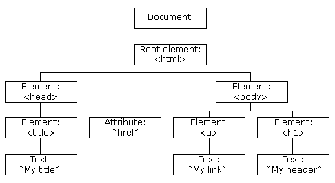
- The DOM is an upside-down tree structure with the root at the top as seen in Figure 7.1. (Docs 2023)
- Each node corresponds to an element, text node, or attribute.
- All of the properties, methods, and events available for manipulating and creating web pages are organized as objects.
- Parent–child relationships define containment and scope of the nodes.
- Browsers parse the DOM to figure out how to organize the objects for presentation in the browser.
Even though not every node is an HTML element (some are text or attribute nodes), it’s common to refer to the all the nodes in the DOM as elements.
- You will see the term “elements” used to refer to “nodes” regardless of the actual node type.
Scraping libraries in both R and Python work by navigating and querying this DOM tree to find the elements with the content of interest you want to extract.
7.5.3 HTML Elements
Each HTML element consists of:
- A tag name (e.g., div, span, a, h3)
- Optional attributes (e.g., id, class, href, data-*)
- Content (text or nested elements)
When you scrape an HTML document, and convert it into text, you will see the HTML tags marking up the text.
- These tags (always in pairs for begin and end) delineate the nodes in the document, the internal structure of the nodes, and can also convey formatting information.
- There are over 100 standard HTML tags. Some commonly used tags are shown in Table 7.1.
Attributes, especially class, id, and data-* attributes, are often the most stable information for identifying content you want to extract.
7.5.4 CSS Selectors
Every website is formatted with CSS.
In CSS rule syntax, the part before the curly brace is called a selector.
- The selector identifies the HTML elements to which the formatting rules should apply.
- These two rules correspond to the following HTML elements:
- The code inside the CSS curly braces consists of the formatting properties and their values.
- The
h3rule applies to all<h3>elements, making their text red and italic. - The second rule applies to all
<div>elements with class “alert” that are descendants of a<footer>element, hiding them from view.
- The
- CSS applies the same formatting properties to every element matched by the selector.
- Each
h3tag will be styled in red, italicized text.
- Each
- The term “cascading” in CSS refers to how formatting rules are inherited and resolved.
- Styles applied to a parent element may propagate to its children.
- When multiple rules apply, CSS uses a priority system (specificity, order, and importance) to determine which rule takes effect.
There are five categories of CSS selectors
- Simple selectors select elements based on tag name, id, or class.
- A tag (element) selector uses the HTML tag name, such as
h3.- All
<h3>elements in the document will be selected.
- All
- An
IDselector uses#, for example#my_id, to select the single element withid="my_id".- IDs are intended to be unique within a page.
- A
classselector uses., for example.my_class, to select all elements withclass="my_class".
- A tag (element) selector uses the HTML tag name, such as
- Combinator selectors combine simple selectors to narrow the set of selected elements based on a relationships between elements in the DOM.
- As an example,
my_name.my_classselects elements with tag namemy_nameand classmy_class. - The most important combinator for scraping is whitespace, ` ` which represents the descendant relationship.
- For example,
p aselects all<a>elements that are descendants of a<p>element in the DOM tree.
- As an example,
- Attribute selectors select elements based on the presence or value of an attribute.
- For example,
[attribute_name*="my_text"]selects elements whose attribute name value contains “my_text”. - This is especially useful when class names are unstable but attributes contain consistent identifiers.
- For example,
- Pseudo-class selectors select elements based on a state, such as hover or position.
- Pseudo-element selectors select and style part of an element.
In CSS selectors, a space and a dot mean very different things.
The space, ` ` as in .parent_class .child_class indicates a descendant relationship in the DOM tree: Select any element with class child_class that appears anywhere inside an element with class parent_class.
- The selected element with
child_classdoes not need to share the parent’s class, it only needs to benested somewhere inside the parent element. - The relationship is structural, not visual.
- This is the most common and useful pattern for layout-oriented scoping in scraping.
The Combinator . with no space means the element must have both classes: Select elements that have both class parent_class and class child_class.
- The element is not required to be nested inside anything.
- The relationship is descriptive, not hierarchical.
- This is common when developers layer multiple classes on the same element, for example:
- one class for layout (.card),
- one class for styling (.highlighted),
- one class for state (.active).
When to use which?
- Use descendant selectors (space) when you want to scope extraction to a region of the page.
- Use combined class selectors (no space) when you want to target a very specific element type, and match elements that intentionally carry multiple class labels.
XML Path Language (XPath) is a query language for navigating and selecting nodes in the DOM tree based on structure, relationships, and attributes, rather than fixed visual or positional paths.
These path expressions look very much like the path expressions you use with traditional computer file systems.
CSS selectors and XPath expressions are both query languages over the DOM, but XPath provides more explicit control over tree navigation and node relationships.
When scraping, CSS selectors are re-purposed to query the DOM, even though they were originally designed for styling, not data extraction.
- In practice, web scraping often uses simple, combinator, and attribute selectors.
- These selectors provide substantial flexibility for identifying elements of interest, but their robustness depends on how stable the underlying HTML structure is.
- Selector choice is a trade-off between precision and robustness and understanding selector types helps you choose wisely.
- Thinking in terms of DOM structure vs. class membership helps choose the right form and avoid subtle over- or under-selection errors when scraping.
CSS selectors (and XPath expressions) are queries about the current DOM, not fixed paths to content.
- They describe which elements to select, not where elements are located visually.
- A selector that works today may fail if the underlying structure changes, even if the page “looks” the same.
- This distinction is central to understanding why scraping strategies must prioritize stability over convenience.
7.6 A Web Scraping Workflow
Modern web scraping is best understood as a workflow than as a single act of “finding the right selectors.”
- Users check results and make decisions at each step to adjust their approach.
The core steps in a web-scraping workflow are language-independent:
- Request: make an HTTP request to a web site for a resource
- Response: receive a server response (HTML, JSON, error, redirect, etc.)
- Parse: interpret the response into a structured in-memory representation
- Extract: select and transform the relevant content into data values
- Normalize and align: reshape extracted values into a consistent structure
- Clean and validate: prepare the data for analysis and confirm correctness
Most “scraping problems” are not bugs in the code, but failures, or unexpected behavior, at a specific stage in this workflow.
At a high level, most scraping workflows interact with three conceptual layers of a website:
- The HTTP layer, which governs how requests are made and responses are returned.
- The HTML layer, which defines the document structure and content returned by the server.
- The rendered page, which is what a human sees after the browser executes JavaScript, applies styles, and inserts dynamic content.
Web scraping code sends requests through the HTTP layer to interact primarily with the HTML layer, not the rendered page.
- Many scraping failures occur when assume these layers behave with our automated scraping code like they do with a browser driven by an interactive human user.
7.6.1 Strategies for Using the Workflow
Effective Web Scraping strategies follow the steps in the workflow.
- This is more efficient as errors in earlier steps can make debugging in later steps ineffective.
Best Practice web scraping strategies are generally language independent.
- We will use {rvest} in the to address the different strategy examples but the same strategies apply if using Python.
We will focus on two different web sites to start.
- The United Nations web page titled Deliver Humanitarian Aid
- This is a site focused on maximizing access to its content.
- It is a static page that is fairly stable.
- The IMDb page for the Top 100 Greatest Movies of All Time (The Ultimate List)
- IMDb is a more modern site that balances performance (dynamic loading) with protecting its content.
- The page may may block or alter responses when it detects automated clients, add content after initial loading, and deliver partial content.
- The website structure is frequently changed and updated.
7.7 Check for Valid Requests
All web-scraping workflows begin with an HTTP request, even when this is abstracted away by a high-level function such as rvest::read_html().
At this stage, the goal is simple: Receive the intended resource from the server in a form that can be parsed.
Key considerations at the request stage include:
- Target the correct URL
- Confirm you are requesting the canonical page (the real URL), not a redirect, preview, or mobile variant.
- Developer Tools and page metadata can help identify the canonical URL.
- Present a reasonable client identity
- Many modern sites distinguish between browsers and automated clients.
- Setting a browser-like User-Agent can prevent soft blocking or alternate responses.
- Minimize unnecessary requests
- Repeated requests during development can trigger rate limits or gating.
- Once access is confirmed and the response looks correct, save the response locally and work from that copy.
At this stage, you are not selecting elements or extracting data yet. Instead, you are answering: Did the request succeed?
- Common failure modes include status codes 403 (blocked), 429 (rate limited), other non-200 responses, redirects (to other pages), and “interstitial pages” (pages about permissions instead of site content).
- Interstitial pages are pages focused on controlling or mediating access to the page (sometimes called “intermediary pages”).
- They may enforce consent requirements, verify the client, or deter automated access.
- From a scraper’s perspective, these pages often return valid HTML but do not contain the expected content.
- Web sites may use Cookies to control consent state, personalization, or to manage access (access gating or token gating).
- Most scraping packages manage cookies automatically within a session.
- However, cookies can still influence what HTML you receive, even when the HTTP status code is 200.
Both general access gating and more specific token gating are mechanisms for controlling who can access content, but they differ in how access is verified and where the decision is enforced.
Access gating controls access based on request context and client behavior.
- Enforcement is typically server-side and stateful.
- Decisions are based on: Cookies (consent, session state), Headers (User-Agent, language, region), IP reputation or request patterns, and JavaScript challenges or interstitial pages
Access gating is common on public websites that want to be: discoverable by search engines, usable by humans and resistant to automated scraping or misuse
From a scraping perspective: access gating often returns Status 200 with altered HTML so failures are subtle and can masquerade as successful requests.
Token gating controls access based on possession of a credential or token.
- Enforcement is typically explicit and stateless.
- Access requires presenting a valid token with the request.
- Tokens may include: API keys, OAuth tokens, Signed cookies and even Cryptographic or blockchain-based tokens
Token gating is common for: APIs, paid content, authenticated services, or rate-limited or licensed data access
From a scraping perspective: Token gating usually results in clear failures (401/403) as access is binary: you either have the token or you do not.
7.7.1 Check Your Credentials
Credential errors (in the classic sense) tend to return explicit HTTP status codes such as 401 Unauthorized, 403 Forbidden, or sometimes 407 Proxy Authentication Required.
- These are often accompanied by clear messages like “Authentication required”, “Forbidden”, etc.
- You wont see these in an {revest} response but can use a lower-level HTTP tool (e.g., {httr2} to submit a request and you would see these codes directly.
If you have a credential issue then you verify whether credentials are required at all
- Check the site’s documentation or network behavior to determine whether access is gated by tokens (API keys, login sessions) or by softer mechanisms (cookies, headers, behavior).
- A clear 401/403 error typically indicates missing or invalid credentials rather than a scraping or selector issue.
Confirm that credentials are being sent correctly
- Ensure that API keys, tokens, or session cookies are actually included in the request (headers, query parameters, or cookies as required).
- A common failure mode is having valid credentials available locally but not attached to the outgoing request.
Validate credential scope and freshness
- Check whether tokens have expired, are rate-limited, or are restricted to specific endpoints, IP ranges, or usage patterns.
- Credentials that work for one request or endpoint may silently fail for others if their scope is too narrow.
When access or token gating is involved, failures at the request stage must be resolved before any parsing or extraction strategy can succeed.
7.8 Check Your Access at the HTTP layer: Is the response with a valid DOM (Structural Validation)?
Even when a request succeeds (suggesting an HTTP 200 response), the returned page may still be unsuitable for scraping.
Modern web sites increasingly attempt to detect automated scraping tools using code, e.g., bots or services such as from Browse.ai or scraping bot, instead of humans interacting using real browsers.
They may
- return partial HTML scaffolding,
- return consent or verification pages,
- or serve alternate content to suspected bots.
This is often referred to as soft access gating:
- You are allowed to connect, but,
- You are not given the same HTML a human browser would receive.
A critical next step is therefore to confirm: The HTTP layer returned HTML that parses into a valid DOM representing the intended page.
7.8.1 Set a Browser-like User-Agent
If a response object does not parse into a usable DOM (for example, a missing or invalid root element), a simple and often effective first step is to set a browser-like User-Agent.
This does not guarantee success but it frequently resolves soft access gating.
User-Agent strings identify the browser and operating system making the request.
- Many sites use them as a first-pass check to distinguish real browsers from automated clients.
See the Updated List of User Agents for Scraping & How to Use Them and select one for your code.
- They are matched to browser and operating system versions.
- Using a realistic, up-to-date value is preferable to inventing one.
Here are recent examples.
#Chrome 144 and Mac OS 15.17
user_agent_str <- "Mozilla/5.0 (Macintosh; Intel Mac OS X 15_7_3) AppleWebKit/537.36 (KHTML, like Gecko) Chrome/144.0.0.0 Safari/537.36"

# Chrome 144 and Windows 10/11
user_agent_str <- "Mozilla/5.0 (Windows NT 10.0; Win64; x64) AppleWebKit/537.36 (KHTML, like Gecko) Chrome/144.0.0.0 Safari/537.36"
Most scraping tools provide a mechanism for attaching a User-Agent to outgoing requests.
- Consult the package documentation for the recommended approach.
Make it a routine practice to consider setting a User-Agent early in your scraping workflow—especially when:
- the parsed document has no usable HTML root,
- expected elements are missing, or,
- code and selectors that previously worked suddenly return zero nodes.
Before modifying selectors or extraction logic, always verify that you successfully accessed the HTML layer you intended to scrape.
7.8.2 Structural Validation Examples: UN and IMDb
Listing 7.1 has some quick checks of the response object for the UN page to see if it returns an HTML response with a valid DOM structure we can try to parse.
This example introduces rvest::read_html(), which is a core function for web scraping in R.
read_html()performs the HTTP request to the specified URL.- It then parses the returned HTML into a document object using the {xml2} package.
- The result is an in-memory representation of the page’s DOM (if it was returned) that we can inspect and query.
- We also use a few {xml2} helper functions to examine structural properties of the returned document.
# 1) Define the target
url <- "https://www.un.org/en/our-work/deliver-humanitarian-aid"

# 2) Attempt to read the page
doc <- read_html(url)

# --- Did read_html() return something parseable? ---

# 3) Check the document object
str_glue("Class Object: ", str_c(class(doc), collapse = "-"))

# 4) Check for a root node
root <- xml2::xml_root(doc)
str_glue("Class Root: ", str_c(class(root), collapse = "-"))

# 5) Check the root node type and name
str_glue("Type Root: ",xml2::xml_type(root))
str_glue("Name Root: ",xml2::xml_name(root))- There is a response so there does not appear to be a credential issue.
- The
docis an xml_document with a valid root node. - The root node is an HTML element (Name Root: html).
- The request successfully reached the HTML layer, returned a complete static page, and produced a usable DOM with a valid structure so we can now try to parse to see if the content is the correct page.
Listing 7.2 uses the same quick checks as Listing 7.1 but with the URL for the IMDb page to see if it returns an HTML response with a valid DOM structure we can try to parse.
# 1) Define the target
url <- "https://www.imdb.com/list/ls055592025/"

# 2) Attempt to read the page
doc <- read_html(url)

# --- Did read_html() return something parseable? ---

# 3) Check the document object
str_glue("Class Object: ", str_c(class(doc), collapse = "-"))

# 4) Check for a root node
root <- xml2::xml_root(doc)
str_glue("Class Root: ", str_c(class(root), collapse = "-"))

# 5) Check the root node type and name
str_glue("Type Root: ",xml2::xml_type(root))
str_glue("Name Root: ",xml2::xml_name(root))- There is a response so there does not appear to be a credential issue.
docis returned as an xml_document, but- the root node is xml_missing.
- The root node has no type and no name (
NA).
Although read_html() returned an object, the response did not parse into a valid HTML document tree.
- This indicates the request did not reach the intended HTML layer to return a valid DOM.
7.8.3 Creating a Session Example: IMDb
If the response is being blocked from the HTML layer, a good next step is to add a non-default user agent to your request to better identify your request.
Do this in R by creating an {rvest} session and setting a browser-like User-Agent for the session.
- A session behaves more like a browser client.
- It lets you set a request identity (User-Agent) explicitly.
- It is the natural starting point for scraping multiple pages later, because the session can carry cookies and other states forward.
Let’s try again by creating a session and setting the user agent for the session.
- We create a session object and attach a browser-like User-Agent to it.
- The session represents a browser-like client rather than a one-off request.
- The same session object can be reused for multiple requests later, since it preserves session state (such as headers and cookies).
This approach keeps request configuration explicit while avoiding repeated setup for each page we scrape.
#Chrome 144 and Mac OS 15.17
user_agent_str <- "Mozilla/5.0 (Macintosh; Intel Mac OS X 15_7_3) AppleWebKit/537.36 (KHTML, like Gecko) Chrome/144.0.0.0 Safari/537.36"

# Chrome 144 and Windows 10/11
#  user_agent_str <- "Mozilla/5.0 (Windows NT 10.0; Win64; x64) AppleWebKit/537.36 (KHTML, like Gecko) Chrome/144.0.0.0 Safari/537.36"

# 1) Define the target
url <- "https://www.imdb.com/list/ls055592025/"

# 2) Create a session with a browser-like User-Agent, then read the page from the session
sess <- session(url, httr::user_agent(user_agent_str))
doc  <- read_html(sess)

# --- Did read_html() return something parseable? ---

# 3) Check the document object
str_glue("Class Object: ", str_c(class(doc), collapse = "-"))

# 4) Check for a root node
root <- xml2::xml_root(doc)
str_glue("Class Root: ", str_c(class(root), collapse = "-"))

# 5) Check the root node type and name
str_glue("Type Root: ",xml2::xml_type(root))
str_glue("Name Root: ",xml2::xml_name(root))- There is a response so there does not appear to be a credential issue.
- The
docis an xml_document with a valid root node. - The root node is an HTML element (Name Root: html).
- The request successfully reached the HTML layer, and returned a usable DOM with a valid structure so we can now try to parse to see if the content is the correct page.
7.9 Check the Initial Response Object - Is it the right page (Semantically Valid)?
Now that you have a valid object, the next step is to confirm you received the page you think you requested.
Even when a request “succeeds” the response may be a redirected page, or a partial/dynamic scaffold missing all the content you want.
- Inspect the page title.
- Check for the presence of a key phrase you expect.
- Count how many target nodes are present.
- Look for telltale phrases indicating consent or bot pages.
- Treat HTML that is “too small” or missing key sections as a warning sign of blocking or interstitial gating.
- Treat HTML that contains scaffolding but not the data as a warning sign of dynamic loading.
7.9.1 Minimal R Template for Sanity Checks
Listing 7.4 provides some examples of quick checks you can make on a response object to see if it has content for the page of interest.
Let’s start with the UN web page.
- We expect the checks to pass with this page.
We need to set three values for this particular page as part of running the checks.
- The URL
- A “must-have” phrase we expect to see based on our selector
- At least one CSS selector of interest. (We’ll cover how we identified this later on)
The code in Listing 7.4 moves beyond structural validation and performs lightweight semantic validation of the parsed HTML document.
These steps use core {rvest} helper functions that operate on the DOM representation returned by read_html().
html_element()selects the first matching element in the document for a given CSS selector.html_elements()selects all matching elements and returns them as a node set.html_text2()extracts the visible text content from an element or document, collapsing whitespace and removing markup.
Together, these functions allow us to verify the page content matches our expectations before proceeding with more detailed extraction.
url <- "https://www.un.org/en/our-work/deliver-humanitarian-aid"
must_have <- "Deliver humanitarian aid"
css_target <- ".col-sm-12.grey-well"

doc <- read_html(url)

# 1) Page title
page_title <- doc |>
  html_element("title") |>
  html_text2()
str_glue("Page Title: ", page_title)

# 2) Must-have phrase (choose something you expect on the real page)
has_phrase <- doc |>
  html_text2() |>
  str_detect(fixed(must_have, ignore_case = TRUE))
str_glue("Has Phrase: ", has_phrase)

# 3) Count target nodes (replace with your selector)

n_target <- doc |>
  html_elements(css_target) |>
  length()
str_glue("Target nodes: ", n_target)

# 4) Interstitial / gating phrase scan
gate_phrases <- c(
  "cookie", "consent", "privacy", "gdpr",
  "verify you are human", "captcha",
  "access denied", "unusual traffic", "just a moment"
)

page_text <- doc |>
  html_text2() |>
  str_to_lower()

gate_hits <- gate_phrases[str_detect(page_text, str_to_lower(gate_phrases))]
str_glue("Gate Phrase Matches: ", str_c(gate_hits, collapse = "-"))

# 5) Rough size heuristic
n_chars <- str_length(as.character(doc))
str_glue("Page Characters: ", n_chars)

doc_u <- doc
The results are consistent with receiving the intended UN page.
- The page title matches the expected content, indicating that the request returned the correct page rather than an interstitial or redirect.
- The must-have phrase is present (TRUE), confirming that the core content of interest appears in the response.
- One target node was found using the selected CSS selector, which is consistent with this page’s structure and sufficient for continued extraction.
- The presence of the word “privacy” in the gating phrase scan is not unexpected for a UN page and does not, by itself, indicate an access problem. Importantly, no stronger indicators of access gating (such as CAPTCHA or verification language) are present.
- The size of the HTML response is relatively large, which is consistent with a full content page rather than a minimal interstitial or error response.
Taken together, these checks suggest that access at the HTTP layer succeeded and that the response object contains the HTML needed for subsequent parsing and extraction.
Let’s try the the IMDb Page using Listing 7.5.
- All we need to do is update the three items of information and set the session object with user agent
url <- "https://www.imdb.com/list/ls055592025/"
must_have <- "Godfather"
css_target <- ".ipc-title__text"

sess <- session(url, httr::user_agent(user_agent_str))
doc  <- read_html(sess)

# 1) Page title
page_title <- doc |>
  html_element("title") |>
  html_text2()
str_glue("Page Title: ", page_title)

# 2) Must-have phrase (choose something you expect on the real page)
has_phrase <- doc |>
  html_text2() |>
  str_detect(fixed(must_have, ignore_case = TRUE))
str_glue("Has Phrase: ", has_phrase)

# 3) Count target nodes (replace with your selector)

n_target <- doc |>
  html_elements(css_target) |>
  length()
str_glue("Target nodes: ", n_target)

# 4) Interstitial / gating phrase scan
gate_phrases <- c(
  "cookie", "consent", "privacy", "gdpr",
  "verify you are human", "captcha",
  "access denied", "unusual traffic", "just a moment"
)

page_text <- doc |>
  html_text2() |>
  str_to_lower()

gate_hits <- gate_phrases[str_detect(page_text, str_to_lower(gate_phrases))]
str_glue("Gate Phrase Matches: ", str_c(gate_hits, collapse = "-"))

# 5) Rough size heuristic
n_chars <- str_length(as.character(doc))
str_glue("Page Characters: ", n_chars)

doc_i <- doc
The results are largely consistent with receiving the intended IMDb page, but they also reveal important structural considerations.
- The page title matches the expected content, indicating that the request returned the correct page rather than an interstitial or redirect.
- The must-have phrase is present (TRUE), confirming that key textual content associated with the page appears in the response.
- Only 27 target nodes were found using the selected CSS selector, which is fewer than the expected 100 items.
- This suggests some content may be dynamically loaded, partially rendered, or structured differently than anticipated.
- The presence of gating-related terms such as cookie, consent, privacy, and GDPR is common on modern commercial sites like IMDb and does not, by itself, indicate access denial.
- Importantly, there are no stronger indicators of blocking, such as CAPTCHA prompts or explicit verification language.
- The size of the HTML response is very large, which is consistent with a full content page rather than a minimal interstitial or error response.
Taken together, these checks indicate that access at the HTTP and HTML layers succeeded, but that the visible list content is not fully represented in the static HTML.
This strongly suggests the use of dynamic loading or client-side rendering for portions of the page, which affects how extraction strategies must be designed.
7.9.2 Work on a Saved Copy of the Response Object
Once you are satisfied the response parses into a valid HTML document and basic semantic checks look correct, a best practice is to save a copy of the page to disk so you do not have to repeatedly re-request it from the website.
- Save the raw HTML response to disk (locally or cloud).
- Use the saved copy while developing and debugging extraction code.
- Re-fetch from the website only when you are confident the rest of the workflow is correct, or when you intentionally want refreshed data.
In R, you can write the parsed document back to an HTML file using {xml2}. The code below ensures a ./data directory exists and then saves the page.
library(xml2)

# Create ./data if it does not exist
dir.create("./data", showWarnings = FALSE)

# Choose a descriptive filename (include date if the page may change)
out_file <- "./data/un_deliver_humanitarian_aid.html"
out_file_i <- str_glue("./data/imdb_top_100_{Sys.Date()}.html")

# Save the parsed HTML document
write_html(doc_u, out_file)
write_html(doc_i, out_file_i)
out_file
out_file_i
7.10 Find CSS Selectors for Elements of Interest
Before writing any scraping code, you need to find CSS selectors that identify which elements in the HTML document correspond to the data you want.
- This requires understanding how elements are labeled and organized in the DOM and how to use that structure to identify the elements of interest using the CSS selectors.
There are two complementary approaches:
- SelectorGadget, for fast, interactive discovery of candidate selectors on mostly static pages.
- Browser Developer Tools, for precise inspection of the DOM when pages are more complex or dynamic.
Neither tool is required for programmatic scraping, but both can be useful for understanding the structure of a page before writing code.
7.10.1 Using SelectorGadget with Chrome
SelectorGadget is an open-source extension for the Google Chrome browser.
SelectorGadget is especially useful during exploratory work.
- It helps you quickly identify candidate selectors.
- It does not guarantee a selector is optimal, stable, or complete.
To install SelectorGadget, go to Chrome Web Store.
Once installed, manage your chrome extensions to enable it and “pin” it so to appears as an icon, ![]() , on the right end of the search bar.
, on the right end of the search bar.
- Click on the icon to turn SelectorGadget on and off.
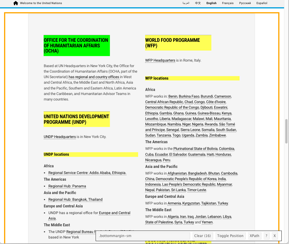
7.10.1.1 United Nations Web Page on Deliver Humanitarian Aid.
Go to Deliver Humanitarian Aid in a Chrome browser.
- Scroll down to the section called Where are the UN entities delivering humanitarian aid located?
Turn on SelectorGadget and click near the edge of the grey box containing the agencies and locations.
- The background should turn green (indicating what we have selected) as in Figure 7.2.
- Other elements matched by the same selector appear in yellow.

SelectorGadget displays information at the bottom of the page:
- It shows the current selector
.grey-wellassociated with the box we clicked on. - It shows the number of elements matched by the selector.
- Toggle Position moves the information bar to the top of the page (or back to the bottom)
- The “XPath” button will pop up the XPath for the same selection
- The
.grey-wellselector XPath is//*[contains(concat( " ", @class, " " ), concat( " ", "grey-well", " " ))]
- The
- The “?” is the help button.
Scroll through the entire page to visually inspect all the selected elements.
SelectorGadget has no knowledge of which element you intend to scrape.
- It doesn’t always get all of what you want, or it sometimes gets too much.
- It can select hidden elements that don’t show up until you actually start working with the data.
- Sometimes not every child element is present for every parent element on the page as well.
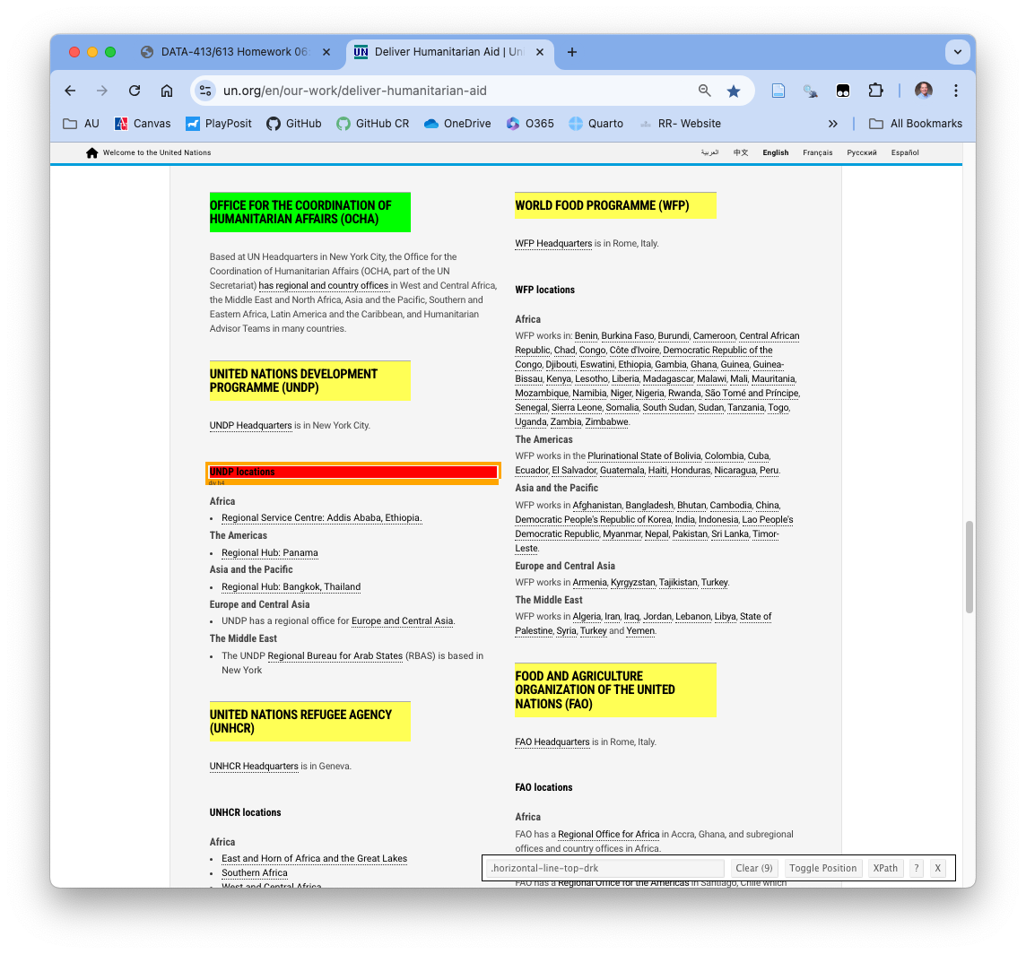
Figure 7.3 shows two elements were matched by the CSS selector and we expected only one.
- If we scroll up we can see another grey-box element highlighted in yellow which means it is currently matched as well (Figure 7.3).
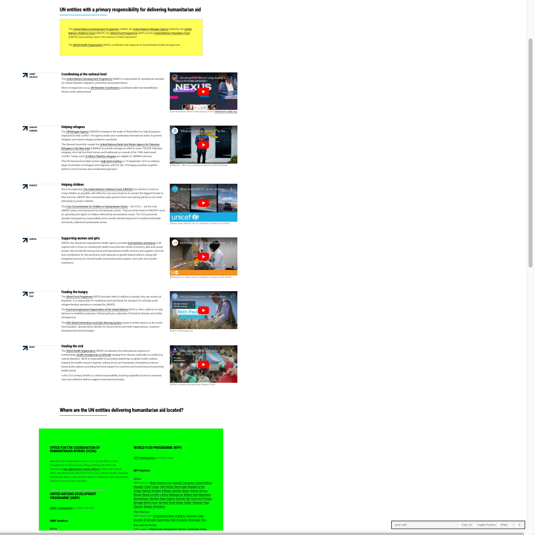
grey-boxes.
- To de-select the yellow grey-box, click on the yellow item we don’t want. It turns red to indicate it is no longer selected.
- However, there is a lot more yellow showing on the page, all elements we do not want.
- Continue to click on the yellow areas until they go away and just the grey box is left in Green and there is no yellow.
- Your screen should look like Figure 7.4 with Selector Gadget showing one item is selected.
- The Selector Gadget selector is now
.col-sm-12.grey-well. - This is more specific CSS selector that matches elements with both class
col-sm-12and classgrey-well. In CSS, writing `.a.b` selects elements that have **both classes a and b, not elements nested inside one another*.- Combining multiple class selectors in this way narrows the match and reduces the chance of selecting unintended elements.
The good news is we now have a CSS selector that identifies the one element of interest.
- However, scraping the whole box at once will give us a lot of text with no clear way to organize it. Let’s try to select individual elements inside the box.
7.10.1.2 Selecting Nested Elements
Often, scraping the entire container (here, the grey box) is not ideal because it produces unstructured text.
Instead, we want to identify repeated sub-elements within the container.
To start over, turn Selector Gadget off and then on (or click on the edge of the grey box to deselect it).
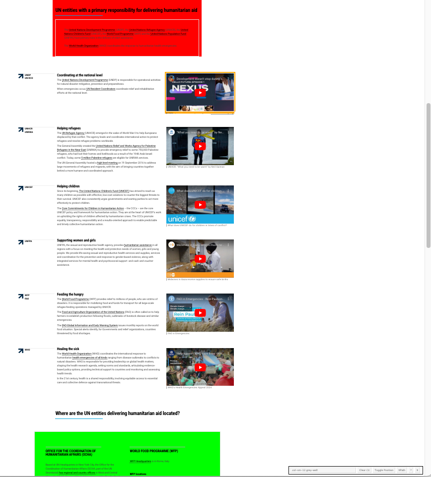
Now click on the edge of “OFFICE FOR THE COORDINATION OF HUMANITARIAN AFFAIRS (OCHA)” inside the grey box.
It should turn Green and other offices should turn yellow. The yellow indicates all the other elements with the same selectors as OCHA. namely,
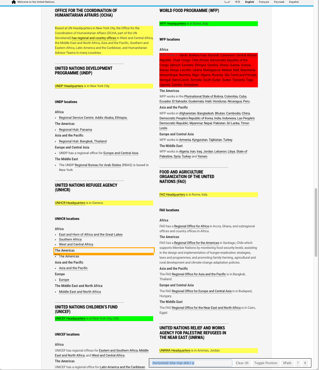
.bottommargin-sm, as in Figure 7.5.Note there are 16 items that were selected.
- However, in addition to selecting the office name element, it selected headings for office locations, e.g. “UNDP Locations”, which we do not want to include with the office names if we can avoid it.
- If we click one of the yellow items we don’t want, it turns red. This indicates we don’t want to select it as in Figure 7.6.
- We now see the selector as
.horizontal-line-top-drkand there are 9 of them which we can verify are correct by scrolling the page up and down.
- One click was all we needed here. On other pages you may need to click several times until only the elements of interest remain in Green or Yellow.
This illustrates a common pattern:
- Start with a broad selection.
- Iteratively remove “false positives.”
- Stop when the selection matches the “elements” you want.
- What are the CSS selectors for the headquarters locations?
- How many elements are selected?
- It takes a few clicks but you can get to just the HQs locations with
.horizontal-line-top-drk+ p. - There should be 9 items.
Selector Gadget can provide a useful tool for understanding the selectors associated with elements of interest on a static web page.
7.10.1.3 When SelectorGadget Is Not Enough
SelectorGadget works best on static pages with visible HTML content.
On more dynamic or heavily scripted pages:
- Clicking may activate links instead of selecting elements.
- SelectorGadget may not identify a stable selector.
- The selector may match elements that are not present in the static HTML.
In these cases, you should switch to the browser’s Developer Tools.
7.10.2 Using Chrome Developer Tools (DOM Inspection)
Modern browser have Developer Tools to help web page developers build, inspect, and test their web pages.
These Browser Developer Tools allow one to inspect the actual DOM tree and examine element names, classes, ids, and attributes directly.
To open the Chrome developer tools
- Use the hamburger menu on the top right
⋮ \> More tools \> Developer tools, or, - Right-click on any element in the web page and select
Inspect.
to get a result as in Figure 7.8.
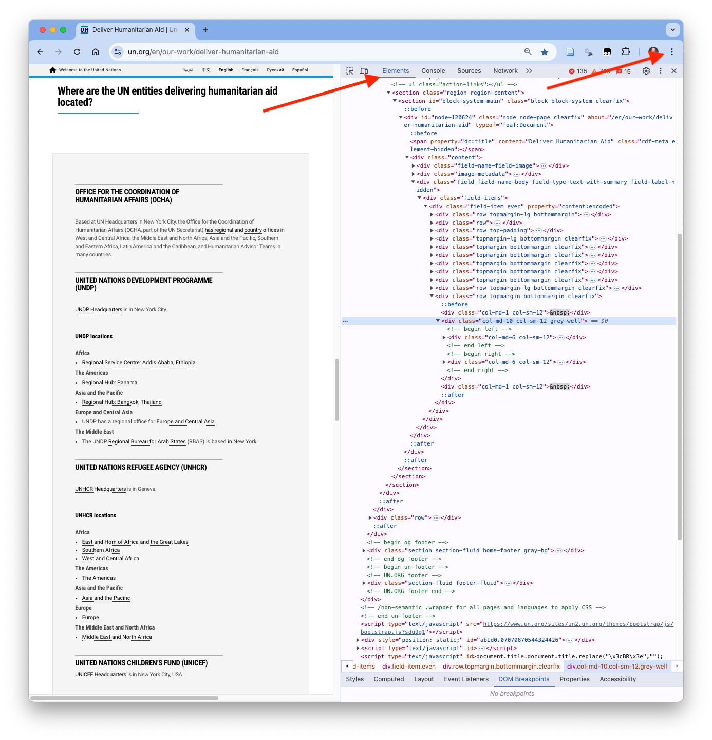
We are most interested in the Elements pane as it shows:
- The DOM tree structure.
- HTML element names (div, h3, p, etc.).
- Attributes such as class and id.
As you move your cursor up and down the DOM tree in the Elements pane, the corresponding region of the web page is highlighted and pop-ups may appear with the CSS for that element.
- If it is unclear where you are, right-click on any element in the web page and select
Inspectand the Elements pane will scroll to highlight the inspected element.
This makes it easier to:
- See how elements are nested.
- Identify stable parent containers.
- Distinguish presentation-related classes from structural ones.
Chrome Developer Tools provide several panes that are useful for understanding how a web page is built and how data is delivered.
Elements: Shows the DOM tree for the page. This is the most important pane for scraping.
- Inspect element names, classes, ids, and attributes.
- Understand parent–child relationships and nesting.
- Identify stable containers and repeated item structures.
Styles: Displays the CSS rules applied to the selected element.
- Helps distinguish structural classes from purely visual ones.
- Useful for recognizing auto-generated or presentation-only classes that may be brittle for scraping.
Console: Allows you to run JavaScript and view messages from the page that may be useful for checking whether content is generated dynamically.
Network: Shows all network requests made by the page which may be useful for identifying JSON payloads, pagination requests, and dynamic data sources when working with live or JavaScript-rendered pages.
Application: Displays cookies, local storage, and session storage which may be useful for understanding consent gates and session-based access.
For static pages, the Elements pane is often sufficient.
For dynamic pages and live sessions, the Network and Console panes become essential tools for diagnosing how and when data is loaded.
As an example, right click on the grey background from before, choose Inspect, and you should see something like in Figure 7.9.
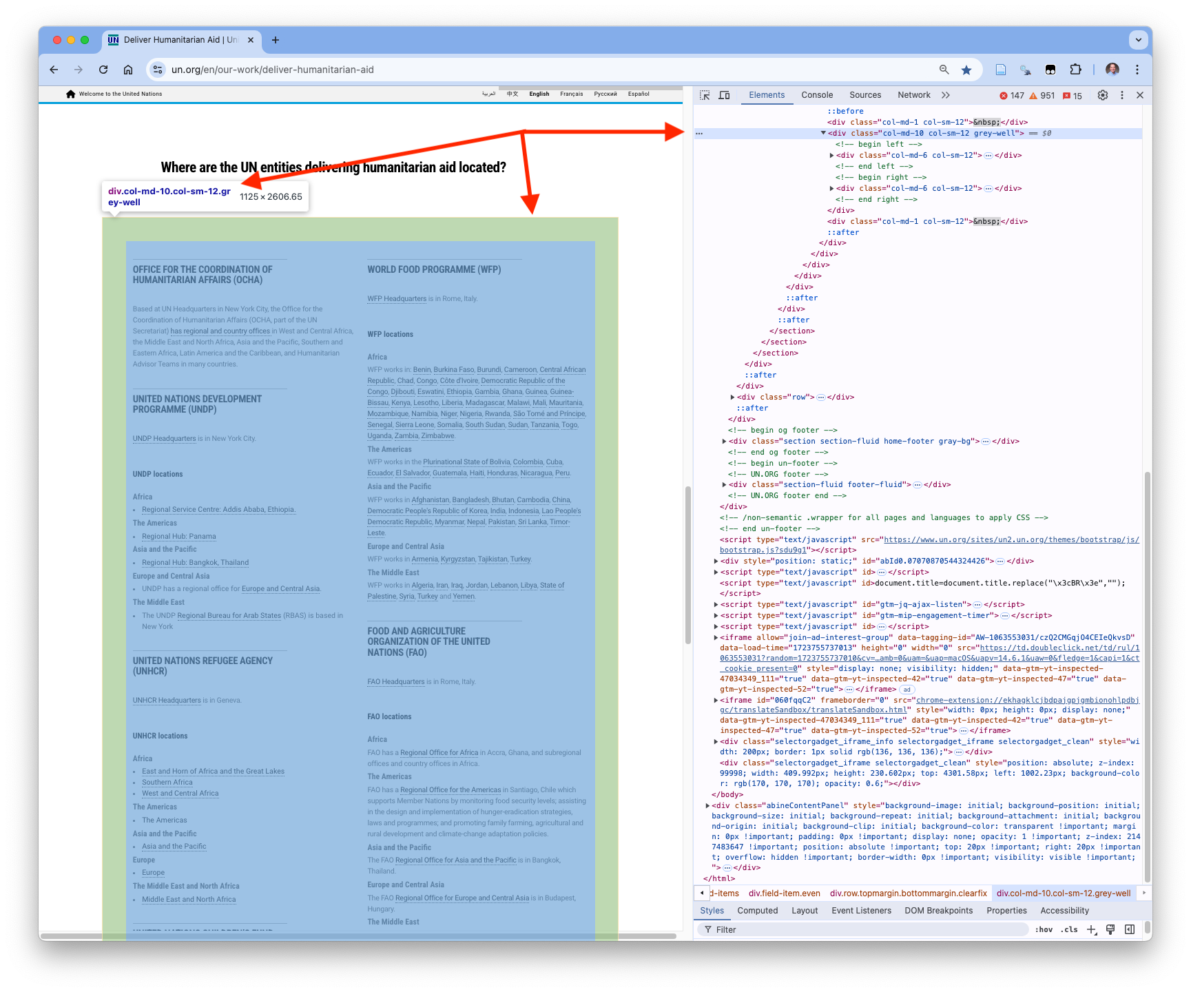
Look for the
name,id,classand other attributes. They may be higher in the tree structure.If the name is the same as the HTML element, e.g.,
divyou will not see a specificname=attribute.Use the arrows to the left of each element to collapse and expand the element to see any nested elements (further down in its branch of the DOM tree).
Right click on a specific element in the Elements pane and you can add or edit attributes of the element (not for us).
You can also:
Copy element: useful for seeing the raw HTML.
Copy selector: often too specific for scraping multiple items.
Copy XPath / Copy full XPath: precise but often brittle paths to a single element.
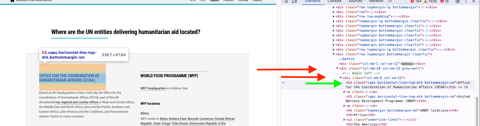
- Use the developer tools to inspect the Title for the OCHA.
- What is the class for it? What is the CSS selector?
- What is the XPath for it?
- Right click on the OCHA title in the web page and Inspect the element or go to the Elements pane and click on the down arrows and scroll till you can see the element (and it is highlighted on the web page) as in Figure 7.10
- You can see the class in the Elements pane, or.
- Right Click and
Copy elementand paste into your file to get<h3 class="caps horizontal-line-top-drk bottommargin-sm">Office for the Coordination of Humanitarian Affairs (OCHA)</h3> - You can see the cascading classing in this. Note that you can pick out the
horizontal-line-top-drkfound by selector gadget earlier. - Add the ‘.’ to the front to designate it as a CSS class selector or
".horizontal-line-top-drk".
- The Xpath and Full Xpath are:
//\*[@id="node-120624"]/div/div\[3\]/div/div/div\[11\]/div\[2\]/div\[1\]/h3\[1\]/html/body/div\[2\]/div\[1\]/div\[1\]/div/section/section/section/div/div/div\[3\]/div/div/div\[11\]/div\[2\]/div\[1\]/h3\[1\]
- Note they are precise but not as useful for our purposes unless we need to select a single element.
- The XPath language can be very flexible though for identifying groups of elements based on locations in the DOM.
7.10.3 How These Tools Fit into the Workflow
- SelectorGadget is best for rapid discovery and hypothesis generation.
- Developer Tools are best for confirming structure and understanding why a selector works (or fails).
- Neither tool replaces careful validation in code.
The goal is not to find a selector, but to find a selector that is:
- Conceptually aligned with the data you want,
- Robust to small layout changes, and,
- Appropriate for repeated extraction.
7.11 Develop Extraction Strategies that Emphasize Stability Over Convenience
Selectors are not the goal. Reliable, maintainable data extraction is the goal.
Modern web scraping succeeds by choosing what layer to extract from and how to anchor that extraction so it remains robust when pages evolve.
- In practice, this usually means preferring strategies that rely on structure and meaning at the HTML layer, rather than what you see at the browser’s interface presentation.
7.11.1 Strategy 1: Extract Content from Element Attributes if possible
When possible, extract data from HTML attributes rather than the visible text.
It is quite common for HTML elements to have attributes that duplicate or partially summarize their visible content.
- This happens most often when the content serves an additional purpose beyond display, such as a navigation link, accessibility, indexing, or interaction with JavaScript.
In practice this means:
- Select the element you care about (often a link, image, or container).
- Extract the attribute values from those elements (for example
href,src,data-*,aria-*).
Attributes are often more stable than visible text because they support core page behavior (navigation, accessibility, SEO), so developers are less likely to change them casually.
Common examples include:
- Links (
<a>)- The visible link text is often paired with a meaningful href attribute.
- The href may contain identifiers or structured information not visible on the page.
- Accessibility attributes (
aria-*,title,alt)- These attributes frequently repeat or paraphrase visible text to support screen readers and assistive technologies.
- As a result, they often provide cleaner or more complete versions of the content.
- Data attributes (
data-*)- Developers often store canonical or machine-readable values in attributes while rendering a formatted or abbreviated version as visible text.
- Metadata (
<meta>,<link>)- These elements may contain information that is not directly visible on the page but represents the same underlying content (e.g., page titles, descriptions, canonical URLs).
Attribute-first extraction is frequently more stable than scraping visible text since the attributes often support core functionality (navigation, accessibility, SEO).
- Developers are less likely to rename or remove them casually.
- They can exist even when visible text is dynamically generated.
In the IMDb example, each movie title is wrapped in an anchor <a> tag whose href contains the movie’s unique identifier.
- The
hrefoften contains a stable title identifier (for example anhref = "/title/tt.../ path"), which is usually more stable than the surrounding layout or text.
However, it is not safe to assume that every element will expose its content in attributes.
- Some attributes contain only identifiers or flags.
- Some content exists only as rendered text.
- Some attribute values may be incomplete or intentionally abbreviated.
For scraping, the practical rule is:
**Always inspect both the visible text and the attributes of candidate elements, and prefer attributes when they provide a stable, structured representation of the same information.*
Attribute-first extraction is a strategy for robustness, but not something you can always do for all the content of interest.
7.11.2 Strategy 2: Layout-Oriented Scoping (Page-Region Selection)
The first step in stable extraction is often to limit the scrape to the section of the page layout that contains the content of interest.
Modern pages frequently include multiple regions that share similar classes or elements, such as:
- navigation menus,
- sidebars,
- promotional panels,
- “related content” sections,
- footers.
Layout-oriented scoping means excluding unrelated regions so you can focus on the content of interest before attempting fine-grained extraction.
- Identify a container element (often a
<div>) that defines the relevant page region, e.g., in Section 7.10.1.1, the.col-sm-12container for the UN box with the grey background. - Use that container as the leading (leftmost) part of your selector, when helpful, e.g.,
.col-sm-12.grey-well.
At this stage, the goal is not to extract individual fields, but to answer: Which part of the page should I scrape at all?
Example (conceptual): Instead of selecting .ipc-title__text globally across the DOM, scope it to a layout region: .main-content .ipc-title__text
- This reduces accidental matches from headers, side panels, or repeated page components.
7.11.3 Strategy 3: Logical Extraction Within (Parent–Child) Items
Once the correct page region is isolated, focus shifts from layout to logical structure within the DOM.
Suppose we want to scrape multiple fields from a page where the same CSS selectors repeat. e.g., the titles, rankings, and ratings of movies in the IMDb Top 100 list.
- We can often identify CSS selectors for each individual field.
- However, extracting these fields globally can lead to subtle problems.
- If one movie is missing a rating or year, you may extract 99 values instead of 100.
- At that point, it can be difficult to determine which item is missing data without extensive post-cleaning.
Logical extraction addresses this problem by exploiting the hierarchical relationships in the DOM.
Instead of extracting child elements directly, we:
- extract parent elements that represent complete logical items first, and
- extract child elements relative to each parent.
Logical extraction ensures
- Correct alignment of fields within each item.
- Robust handling of optional or missing child elements as they are correctly associated with their parent.
- Stability when the page layout changes but the item structure remains consistent.
Logical extraction workflow:
- Identify a parent element that represents one logical item (for example, a movie, product, or article).
- It should contain the child elements of interest
- Identify the CSS selector for the parent element and each child element of interest.
- Extract all the parent elements first.
- For each parent element, extract child elements using selectors scoped within that parent (parent CSS as the left of the CSS selector for each child, separated by a space).
- If a child element is missing for a given parent, record its value as
NA.
This strategy is also know as anchoring but this does not refer to the HTML <a> (anchor) tag.
- Anchoring means scoping selectors to a stable parent element in the DOM, so child selectors match elements only within the intended logical context.
You should always validate the result using element counts and spot checks and inspection of missing elements.
Anchoring selectors in this way reduces over-selection, improves robustness to layout changes, and makes extraction code easier to understand and maintain.
IMDb example: Anchoring a Parent to a Child selector
- First extract all movie containers using the parent selector
.dli-parent - Then, for each parent (container), extract title, year,, score, link, …. using selectors scoped within that parent.
This parent-first approach is quite helpful when scraping complex pages with repeated, partially optional content.
7.11.4 Strategy 4: Treat Tables as Data
If a page contains actual HTML tables, the scraping package may provide functions specifically designed to extract tabular data rather than working with plain text.
rvest::html_table()works well with well-formed, nearly rectangular tables, returning the result directly as a tibble.- This is usually much faster and more reliable than scraping text and manually restructuring it into rows and columns.
- Header rows, column alignment, and basic type coercion are often handled automatically.
That said, table-based extraction still requires care:
- Table structure can vary across pages (missing columns, extra header rows, merged cells).
- Column names and ordering may differ slightly between tables.
- Normalization is often required before combining tables from multiple pages.
When available, HTML tables are often the most convenient and least brittle source of structured data, but you should still validate shape, column meanings, and consistency before analysis.
If your target page contains clean HTML tables:
- In R: use
html_table(). - In Python: try
pandas.read_html()first.
If tables are irregular, nested, or mixed with non-tabular content:
- Use DOM-based extraction ({rvest} or BeautifulSoup) at the table element level and build the table manually.
Stable scraping depends more on understanding page structure than on the language or library used.
7.12 From Page Access to Data Extraction: A Practical Workflow
Once you have confirmed access to a page and verified it returns a valid HTML document, the focus shifts from requesting content to extracting data.
- While the underlying concepts are language-independent, we will use {rvest} (with {xml2}) in the examples to demonstrate the workflow in R.
At this stage, a best practice is to work from a saved copy of the page rather than repeatedly requesting it from the website.
- This avoids unnecessary network traffic and rate limits, makes your work reproducible and separates extraction logic from access and gating issues.
In the sections that follow, we assume:
- The HTML page has already been retrieved successfully, e.g., with
read_html(url)orread_html(sess) - A local copy of the page is available on disk.
- We are working purely at the HTML / DOM layer.
Before writing extraction code, you must identify the selectors for the parent containers and child elements of interest, guided by the extraction strategies described earlier (layout scoping, logical parent–child structure, attributes, tables, or embedded data).
- When tables are present, prefer table-aware extraction; otherwise, select and extract child elements relative to their parent containers to preserve alignment and robustness.
The basic workflow revisited:
- Use
read_html()to access the HTML document (from a URL, an HTML file, or an HTML string) to create a copy in memory.- Since
read_html()is an {xml2} function, the result is a list object with classxml_document.
- Since
- Use
html_element(doc, CSS)orhtml_elements(doc, CSS)to extract the element/elements of interest from the xml_document object with the CSS selectors you have identified.- The result is a list object with class
xml_nodeif one element is selected or,xml_nodeset, if more than one element is selected.
- The result is a list object with class
- Extract data from the selected elements using the appropriate helper function:
html_name(x): extract the HTML tag name of the element(s) (xml_document,xml_node, orxml_nodeset)html_attr()orhtml_attrs(): extract one or more attribute(s) of the element(s). The result is always a string so may need to be cleaned.html_text2(): extract the text inside the element with browser-style formatting of white space orhtml_text()for original text code formatting (which may look messy).html_table(): extract data structured as an HTML table. It will return a tibble (if one element is selected) or a list of tibbles (when multiple elements are selected).
This workflow provides a consistent foundation for extracting, restructuring, and validating data from web pages using R.
The following examples demonstrate how the extraction and strategies fit together.
7.13 Example 1: Scraping a Static Page (UN Humanitarian Aid)
For reproducibility (and to avoid unnecessary requests), we will work from the HTML file we saved earlier.
- When reading from disk, you are working entirely at the HTML/DOM layer and are insulated from changes in access gating, rate limits, and the page DOM that may have occurred since you downloaded the file.
- When done, you can create and save a new file to confirm the code still works.
- Load the Saved HTML file
Use read_html() to read from a URL, a file path, or an HTML string.
- Extract Elements from the Saved Document
We can use Selector Gadget to find the selector for the box with the grey background is
".col-sm-12.grey-well"Use
html_element()when you expect one match, andhtml_elements()when you expect multiple matches.- We expect one box
- Extract Text from the Selected Element
html_text2()returns browser-style normalized text (typically what you want for scraping).
We have “scraped” the data of interest and converted it into a character vector.
- However, as suspected, it is a lot of text with only new line characters to indicate any kind of structure It would take a lot of cleaning to figure this out.
Instead, let’s try selecting individual elements to see if that is better.
- Use the CSS selectors for the Office Names and their HQs locations and extract the text for those elements.
- You should get a character vector of 9 + 9 = 18 elements.
- Convert into a tidy data frame.
- Approach 1. Scrape each individually and combine into data frame (works here because both vectors are complete and aligned).
- Approach 2. Extract together, then reshape (more general when you extend to more fields).
html_elements(un_html_obj,
1        css = ".horizontal-line-top-drk, .horizontal-line-top-drk+ p") |>
2  html_text2() |>
3  tibble(un_text = _) |>
4  mutate(
    office_id = rep(1:9, each = 2),
5    id = if_else(row_number() %% 2 == 1, "office", "location")
    ) |>
6  pivot_wider(names_from = id, values_from = un_text) |>
7  select(-office_id)
un_aid_offices - 1
- Combine the two (or more) selectors into a character string separated by commas.
- 2
- Extract the text as a character vector.
- 3
-
Convert the vector into a tibble with column name
un_text. - 4
- Add a column to uniquely identify each pair of office and location.
- 5
-
Add a column
idwith what will be the new column names. - 6
-
Pivot wider based on the new column names column and
un_text. - 7
-
Remove the
office_idas no longer needed.
Now that you have a tidy tibble, you can clean the text as desired, e.g.,
7.14 Example 2: Scraping a Modern Site (IMDb)
This example enables us to practice:
- Identifying CSS selectors using the Developer Tools
- Recognizing the potential for Layout-oriented Scoping
- Recognizing when classes are absent or brittle and need parent context
- Using Parent-element alignment for item-level extraction (Logical Extraction)
- Identifying when “only the first N items are present” due to infinite scroll
- Considering Embedded Data
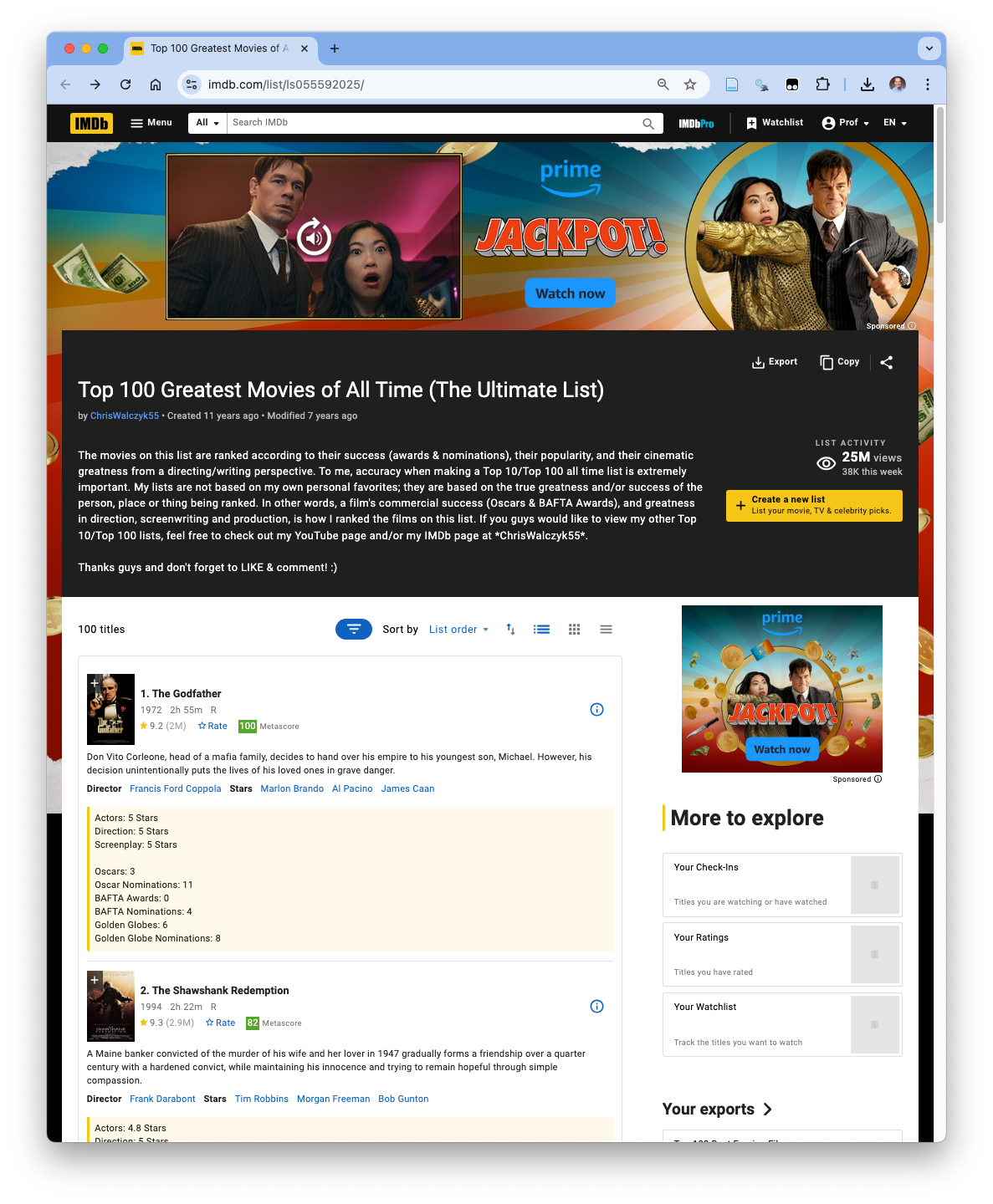
We want to scrape data about the top 100 greatest movies of all time from IMDB (per Chris Walczyk55).
- The URL: https://www.imdb.com/list/ls055592025/ shows a page that looks something like Figure 7.11.
- We are pretending IMDB did not add an export option to download all the data in a spreadsheet….
7.14.1 Load the Saved HTML page
We saved the page as an HTML file so we can now read it in with read_html("path/filename")
The web page R object is an R list where the $head and $body elements contain pointers to the elements in the parts of document.
- The web page document is the top level, single node, for the page so the parent class is
xml_nodeinstead of"node_set".
We can extract the element name and the attributes for the page as well.
We want to get the data for each of the 100 movies for the following elements
- Rank
- Title
- Metascore
- Year
- Votes
7.14.2 Identifying CSS Selectors with Selector Gadget
7.14.2.1 Rank and Title
When we start Selector Gadget and try to select the ranking alone, SelectorGadget does not isolate it cleanly.
- Instead, it consistently highlights the rank and title together as a single text block.
- In practice, this means our first selector will likely return a combined value such as “1. The Godfather”.
Figure 7.12 shows that the selector ipc-title_text matches 103 items which is more than we want.
- Some of these matches come from other headings or title-like elements elsewhere on the page.
- This is a common failure mode when a class is reused across multiple page regions.
- The fix is layout-oriented scoping: restrict the selector to the region of the DOM that contains only the movie list.
Figure 7.13 shows Selector Gadget can also identify a container element that encloses the movie list.
- However, this still gets use 104 elements (we added the container)
- Looking at the selector in the information box, there a comma between the container class selector and the Rank and Title class selector which in CSS means “either/or” (a union).
- It is matching elements that are the container or the Rank and Title selector, thus the 104.
- To scope the titles within the container, we need a descendant selector:
A B(with a space) matches elements that matchBthat occur anywhere insideA.
- So we replace the comma with a single space.
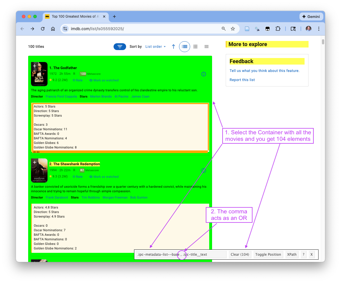
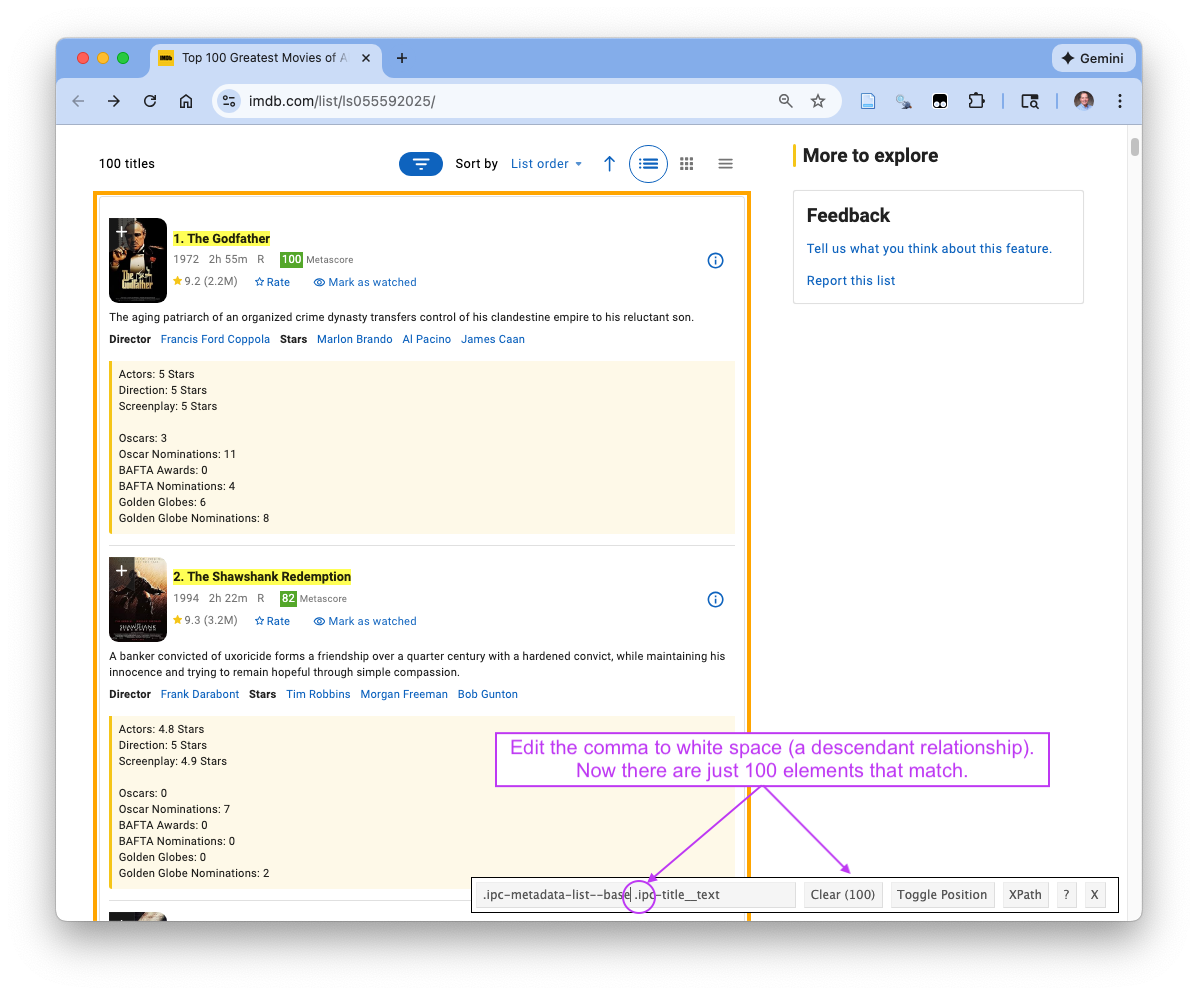
Figure 7.14 now shows that replacing with a single whitespace creates the proper selector that yields 100 elements for the Rank and Title.
- Visually inspect the page to confirm all the movies ranks and title are selected (in green or yellow) and that no unrelated headings are included.
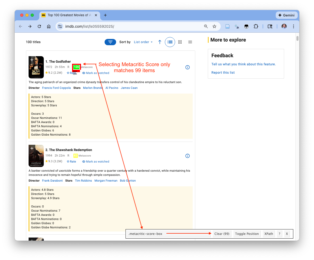
7.14.2.2 Metascore
Figure 7.15 shows SelectorGadget can identify a selector for the Metascore element.
- However, we do not get a clean 100-to-100 match:
- The selector returns 99 elements, which strongly suggests that at least one movie does not have a Metascore element (or it is represented differently for that movie).
- A movie is missing the element but we don’t know which one.
- If we scrape Metascore as a standalone vector, we immediately create an alignment problem: we have no reliable way to know which movie is missing the value.
This is exactly the situation where logical extraction using parent items is safer:
First select the parent element for each movie (one parent per movie).
Then, within each movie parent, extract the Metascore child element (or return NA if it is missing).
Even though the rendered page layout suggests an obvious “movie card” container, the best practice is to confirm the true parent structure in the DOM using browser Developer Tools before committing to the selector.
7.14.3 Identifying CSS Selectors with Browser Developer Tools
Whereas Selector Gadget navigated the DOM behind the scenes using heuristics to identify a selector, we will not navigate the DOM explicitly to find CSS selectors.
- This is a more effective way to integrate the Extraction Strategies from Section 7.11 into our workflow.
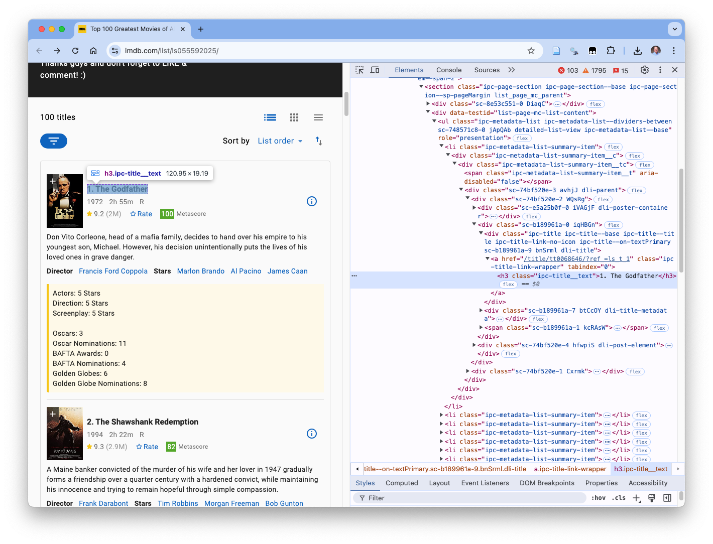
7.14.3.1 Rank and Title
Go to the web page (make sure Selector gadget is off) and right-click on the first movie’s rank (1), and chose Inspect.
Figure 7.16 shows the rank and title are in a single element with class ipc-title__text.
- This explains why Selector Gadget could not identify a selector just for Rank as there was none.
- The Rank number is a text value in the element along with the title.
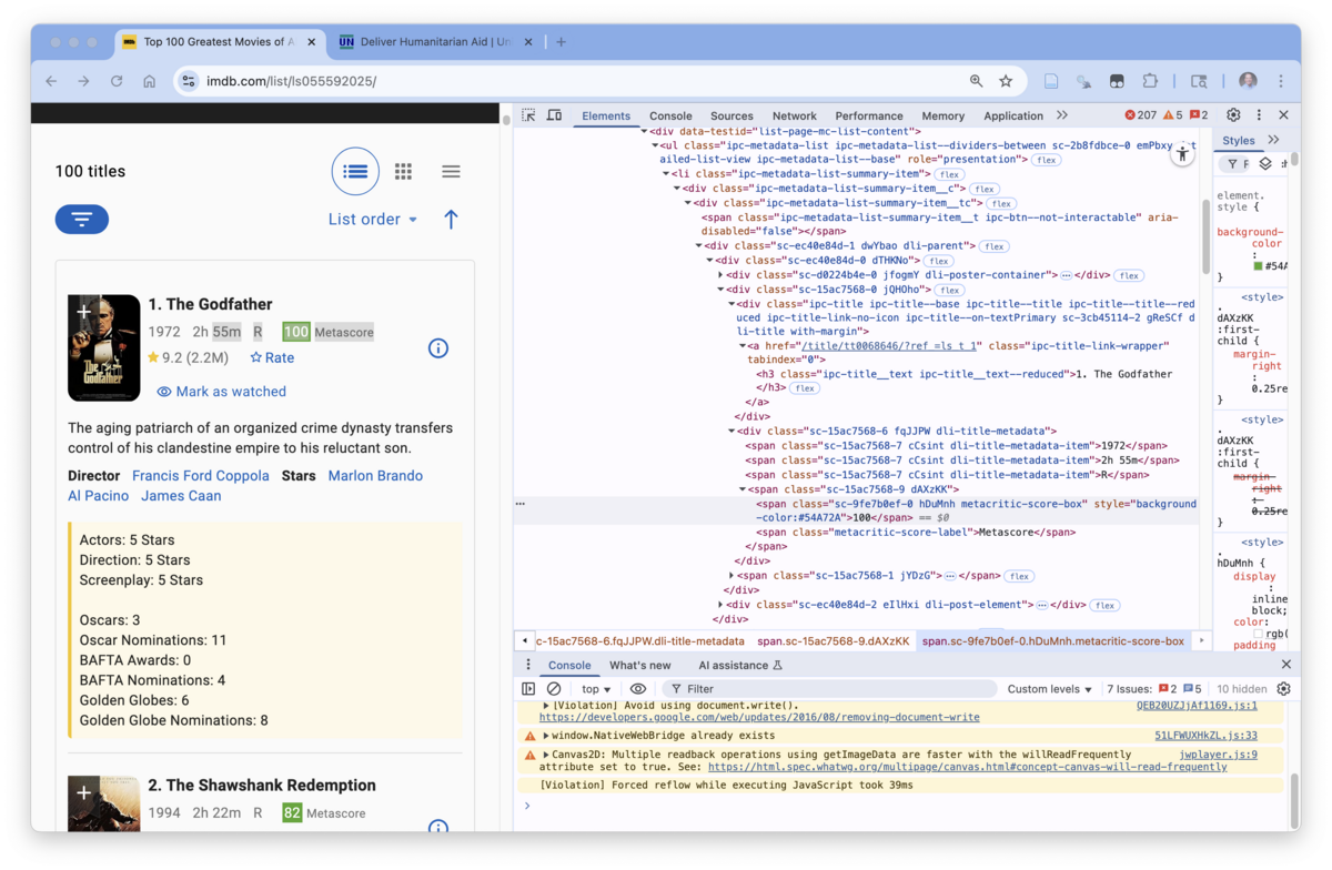
7.14.3.2 Metascore (Logical Scoping)
Figure 7.17 shows that if we Inspect Metascore, it has its own element with class, metacritic-score-box.
- The Selector Gadget CSS selector of
.metacritic-score-boxis accurate. - However, we need to find a parent element for logical scoping since there are only 99 of the elements.
- Inspect the Metascore element on the left to find its line in the DOM in the Elements pane.
- Work your way up the DOM tree element by element.
- As each element is highlighted it may highlight the corresponding element on the rendered page on the left.
- Eventually a “movie” element is highlighted in the rendered page on the left and also highlighted in the DOM tree in the Elements Pane.
Figure 7.18 shows the path from the metascore element to the “movie” element and that the movie element is the parent of metascore.
- Both the pop-up on the rendered page and the element line in the Elements Pane show the class of the movie element is
dli-parent.
When ready to extract we can use the CSS selector for the Parent, .dli-parent, and for the child Metascore, .metacritic-score-box as part of our logical scoping strategy.
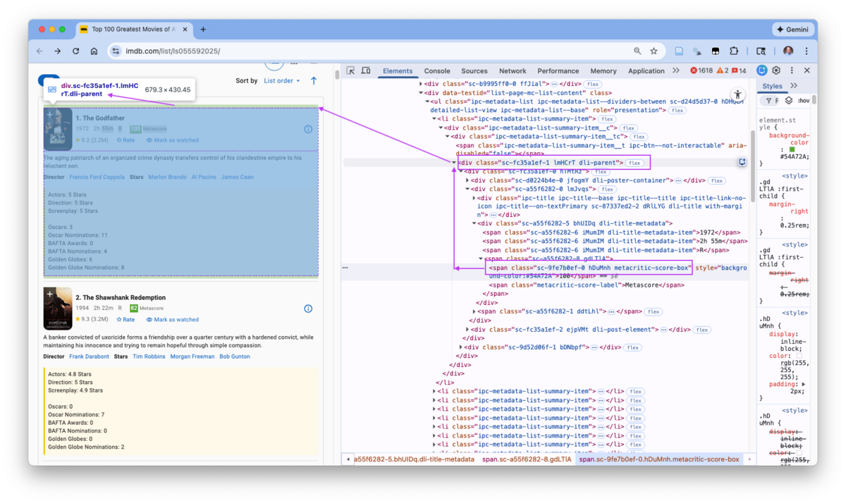
7.14.3.3 Year (Runtime, Rating, and Metascore) (Logical Scoping)
If we used Selector Gadget to find a selector for Year, it would identify the selector .dli-title-metadata-item:nth-child(1).
- This is a positional selector not a semantic one.
- It selects the “first child in the list”, not year.
- If IMDb inserts, removes, or reorders items in this list, the year may no longer be the first element.
- As a result, this selector is brittle and likely to break silently.
Figure 7.19 shows hows why this happens: Year, Runtime, and Rating all share the same CSS class.
- They are visually distinct, but structurally they are peer elements.
- There is nothing in the child element itself that uniquely identifies it as “Year”.
This is a strong signal that scraping the child element directly is risky.
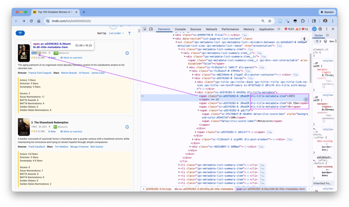
Just above the Year is a div with class dli-title-metadata which is a parent for four items, the year, run time, and rating, as well as metascore.
Figure 7.20 shows the relationship clearly.
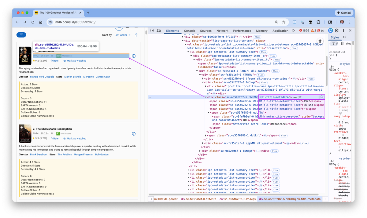
Extracting this parent container is a more robust strategy:
- It preserves the logical grouping of related metadata for a movie.
- It avoids relying on fragile positional assumptions (nth-child()).
- It allows downstream parsing rules to identify year, runtime, and rating based on content patterns rather than DOM position.
This does mean extracting more data than we immediately need, which requires additional cleaning. However:
- Extra cleaning is predictable and visible.
- Broken selectors are silent and harder to detect.
From a scraping perspective, structure-first extraction is safer than position-first extraction, especially when multiple fields share the same class and only differ by meaning, not markup.
7.14.3.4 Votes
If you try to use Selector Gadget for Votes, it will most likely fail with the message “No valid path found”.
- It is not clear here why it is failing on this element
Selector Gadget’s core workflow assumes a relatively “stable” DOM where:
- The nodes you click are the nodes that matter (not wrapped in interactive layers),
- The DOM doesn’t materially change right after load (hydration/infinite scroll),
- Repeated items have consistent markup (no conditional subtrees, no hidden duplicates).
Selector Gadget is useful for quick CSS discovery on static pages, but it was not designed for modern, JavaScript-heavy pages with dynamic DOM and can fail.
Always validate results from Selector Gadget in the Developer Tools.
In this case, Figure 7.21 shows that Votes has its own class, ipc-rating-star--voteCount.
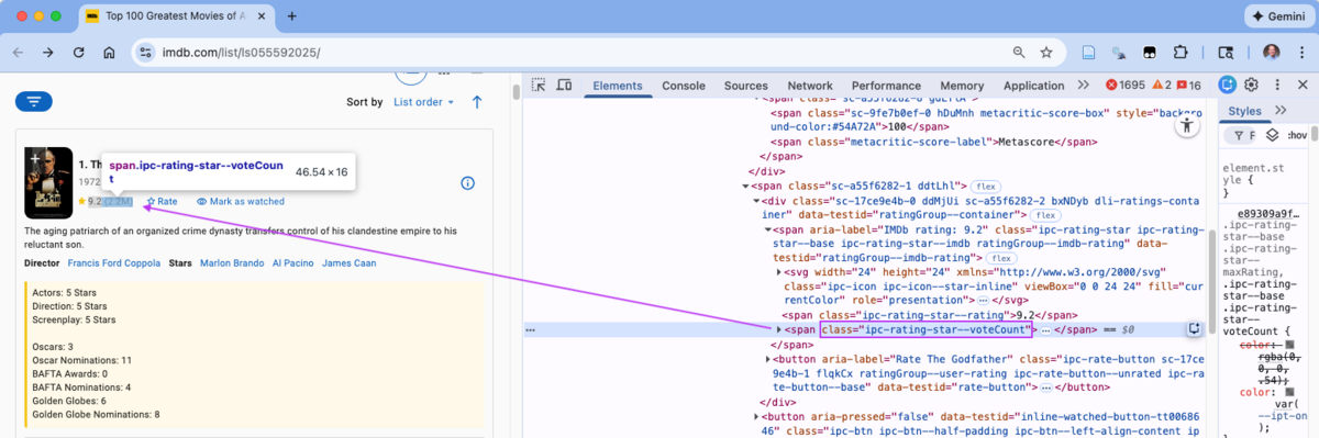
7.14.3.5 CSS Selector Summary
After using Selector Gadget for quick checks and Developer Tools for final identification our extraction strategy can work with the following CSS selectors.
Parent Movie item:
.dli-parentChild elements:
- Ranking and Title:
.ipc-title__text - Metascore:
.metacritic-score-box - Year:
.dli-title-metadata - Votes:
.ipc-rating-star--voteCount
- Ranking and Title:
Each selector is a class selector so begins with the . followed by the class.
7.14.4 Extract the Elements and the Data
Let’s try to extract all the movie elements from our page.
- Recall, when we ran the checks in Listing 7.5, we only got 27 nodes so we should not expect 100 movies.
- IMDb is using a form of infinite scrolling to load the movies after the first 25.
- We have 25 elements which makes sense given the maximum of 25
- We will work on getting the rest once we have confirmed our code can extract the elements we want from these 25 movies.
Since we have four css selectors, let’s build a small helper function to extract the text from an input xml object and a CSS selector.
Now we can put it all together inside a call to tibble() to get the elements using the selectors we identified earlier.
tibble(rank_title = get_text(imdb_movie_elements, ".ipc-title__text"),
        metascore = get_text(imdb_movie_elements, ".metacritic-score-box"),
        year_run_rating = get_text(imdb_movie_elements, ".dli-title-metadata"),
        votes = get_text(imdb_movie_elements, ".ipc-rating-star--voteCount")
) ->
movie_df
glimpse(movie_df)
We now have a nice tibble with 25 rows.
- There is clearly a bit of cleaning to be done but let’s see if we can get all 100 movies first.
- The additional data may generate some additional cleaning requirements.
Since IMDb is using infinite scrolling, we will have to use code to scroll the browser in such a way as to simulate a human.
This requires using a “live session” and a headless browser to simulate the interactions
7.14.5 Example 3: Scraping Dynamic Content with a Live Session (rvest live / chromote)
Use this example to practice:
- Distinguishing “not present in source” from “present but hard to select”
- Scrolling and waiting patterns for lazy-loaded content
- Extracting after rendering, then returning to normal parsing/extraction
Notes:
- Interactive code can succeed while rendered code fails because timing differs.
- Make sleeps explicit, and validate counts after scrolling.
As we have seen, even though we can “see” all 100 elements on a page, they are not really there when the page is first loaded. This is due to the designers using a form of Infinite Scrolling to dynamically load content on the page.
We will have to programatically “interact” with the page to get see as much content as we want. That means using code to simulate as if there were a live user interacting with the page using a mouse or keyboard.
There are several options for interacting with a web page.
- Minimalist approaches require less set up and can handle common actions such as scrolling or clicking.
- Comprehensive approaches allow you to navigating and manipulating interactions with entire web sites. This includes use of the web-site testing capabilities seen with {rselenium} in Section 7.21 or {selenider} in Thorpe (2024).
We will use a minimalist approach of using the {rvest} package.
The {rvest} package includes functions to create a live session and interact with a web page, e.g., read_html_live(). See Interact with a live web page
These functions use the {chromote} package to establish the session and interact with the page. The functions allow you to:
- open a live session in the Chrome browser and use the live session’s methods to
- scroll across the page,
- type text,
- press a key, or
- click on buttons or links.
my_session <- read_htm_live(my_url) creates a session object, e.g., my_session, where the url web page is active.
- The
my_session$view()method is useful for interactive debugging to see what is happening on the page as you execute other methods.- Be sure to comment out for rendering.
- There are several methods to scroll on the page, e.g,
my_session$scroll_by(up.down-pixel, left-right-pixel)can help by scrolling down dynamic pages.- You may need to do several to allow the page to scroll, load, and then scroll again
- The
my_session#click("my_css")moves to a button identified by a css selector and clicks it,- This can be useful when a page has a “load more” button as opposed to dynamic scrolling.
Once you have all the page loaded, you can use html_element() or html_elements() as usual with the my_session object.
7.14.5.1 Example of opening a page and scraping data without moving.
- Remove the comment
#onsess$viewto see it open. You can close the browser tab manually.
library(rvest)
sess <- read_html_live("https://www.forbes.com/top-colleges/")
Sys.sleep(1) # make sure page has time to load
# sess$session$is_active()
# sess$view()
my_table <- html_element(sess,".ListTable_listTable__-N5U5") |> html_table()
row_data <- sess  |>  html_elements(".ListTable_tableRow__P838D") |> html_text()
my_table |> head()
row_data[1:10]
sess$session$close()
7.14.5.2 Example of opening a page and scrolling.
Let’s get the data for 100 movies from the IMDB web page.
Scraping code that works interactively (human typing) may fail during a render process where there is no interactivity. This is because the website may detect the default NULL User Agent and block it (403 error).
To reduce the chances of being blocked, identify your machine by using httr::user_agent() to configure the user agent in the environment as other than NULL.
- Remove the comment
#onsess$viewto see the activity in a Chrome browser tab. You can close the browser tab manually when finished.
library(rvest)

# Define User-Agent string
#Chrome 144 and Mac OS 15.17
user_agent_str <- "Mozilla/5.0 (Macintosh; Intel Mac OS X 15_7_3) AppleWebKit/537.36 (KHTML, like Gecko) Chrome/144.0.0.0 Safari/537.36"

# Chrome 144 and Windows 10/11
#user_agent_str <- "Mozilla/5.0 (Windows NT 10.0; Win64; x64) AppleWebKit/537.36 (KHTML, like Gecko) Chrome/144.0.0.0 Safari/537.36"

# Set global User-Agent
0ua <- httr::user_agent(user_agent_str)

# Start polite live session
1sess <- read_html_live("https://www.imdb.com/list/ls055592025/")
2#sess$view()

# Scroll down slowly to load more movies
for (i in 1:4) {
3  sess$scroll_by(0, 10000)
  Sys.sleep(2)  # Give time for content to load
}

# Extract movie elements
sess |>
4  html_elements(css = ".dli-parent") -> imdb_100_elements

# ---- Save the rendered DOM to ./data ----
dir.create("./data", showWarnings = FALSE)

# Evaluate JS in the page to get the full HTML of the current DOM
5res <- sess$session$Runtime$evaluate(
  expression = "document.documentElement.outerHTML"
)
html_str <- res$result$value  # character string
imdb_path <- "./data/imdb_top_100_movies_live.html"
writeLines(html_str, imdb_path)

6sess$session$close()- 0
- Set the user agent based on OS and Browser. See Updated List of User Agents for Scraping & How to Use Them or similar sources.
- 1
-
Create a new session called
sess. - 2
- Un-comment for interactive work to check if the session is active - useful for interactive debugging.
- 3
- Scroll down the web page as far as needed to load all the elements of interest. In this case, four scrolls of 10,000 pixels each was required. The reason for 4 was to allow the page to load and re-scroll to catch all the movies. Other options may work.
- 4
- Scrape all 100 movie elements using the designated CSS selector.
- 5
-
The next several lines use the low-level browser session
sess$sessionto expose the JavaScript runtime of the page (sess$session$Runtime) and thenevaluate()executes JavaScript inside the browser, exactly as if you typed it in the browser console. The JavaScript expression returns a single character string containing the complete HTML of the page as currently rendered whichwriteLines()saves to the path/filename on disk. - 6
- Closes the session.
Now you can process the data you have collected.
# Build the table
tibble(rank_title = get_text(imdb_100_elements, ".ipc-title__text"),
        metascore = get_text(imdb_100_elements, ".metacritic-score-box"),
        year_run_rating = get_text(imdb_100_elements, ".dli-title-metadata"),
        votes = get_text(imdb_100_elements, ".ipc-rating-star--voteCount")
) -> movie_100_df

glimpse(movie_100_df)
Now we have a tibble with data for all 100 movies and the NA for metascore is for movie 91.
There is still a lot of cleaning to do though which is expected for scraped data.
7.14.5.3 Scrape a Dynamic Page with Chromote
If you need more flexibility than scrolling and clicking, you can try working directly with Chromote.
The {chromote} package uses the open-source Chromium protocol for interacting with Google Chrome-like browsers so you must have Chrome (or a similar browser) installed.
There is limited documentation of {chromote} so may need to search for help on other options.
{chromote} uses what is known as a “headless browser” to interact with a web page.
- A headless browser is a browser without a user interface screen - there is nothing for a human head to see or do.
- These tools are commonly used for testing web sites since without the need to load a user interface, the code can run much faster.
- We can use a
$view()method to create a screen we can observe.
Once the session is established, we can use {chromote} methods to manipulate the page and use {rvest} functions to get the elements we want as before.
Use the console to install the {chromote} package.
To scrape the data we will Load the {chromote} package and do the following
- Create a new session.
- Create a custom user agent. This is not always necessary but can be useful to avoid appearing like a Bot. IMDB will block the default user agent.
- Navigate to the desired web page
- When running interactively, open a browser we can observe.
- Use
Sys.Sleep()to ensure the page loads all the way. Theb$Page$loadEventFired()will suspend R until the page responds that it is full loaded. However, with IMDB it does not respond so we are manually imposing a delay on the next step. - Use a for-loop to scroll down the page while using
Sys.Sleep()to suspend operations so the dynamic content has loaded before scrolling again. This may take multiple loops that you can adjust. - Once you have scrolled to the bottom of the page, use a Javascript function to create an object with the entire page.
- Switch to the usual {rvest} functions to get the html object, scrape the elements of interest, and tidy as before.
- Close the session. This does not close the view you created earlier. You will have to do that.
library(chromote)
options(chromote.verbose = TRUE)

1b <- ChromoteSession$new()
2b$Network$setUserAgentOverride(userAgent = user_agent_str)

3b$Page$navigate("https://www.imdb.com/list/ls055592025/")
# b$Page$loadEventFired()
4#b$view()
5Sys.sleep(.3)
6for (i in 1:6) {
b$Runtime$evaluate("window.scrollTo(0, document.body.scrollHeight);")
Sys.sleep(.3)
}
7html <- b$Runtime$evaluate('document.documentElement.outerHTML')$result$value

8page <- read_html(html)
9imdb_100_elements <- html_elements(page, css = ".dli-parent")
10tibble(rank_title = get_text(imdb_100_elements, ".ipc-title__text"),
        Metascore = get_text(imdb_100_elements, ".metacritic-score-box")
) ->
11movie_100_df

12b$close()- 1
- Start a new session as a tab in a browser
- 2
- For IMDB, and perhaps other sites, create a custom agent to reduce the chance of being blocked as a bot and getting a status code 403 error.
- 3
- Navigate to the web page of interest.
- 4
- Un-comment if you want to see the page in the headless browser - For interactive use only..
- 5
- Use a delay to make sure the page is fully loaded before attempting to scroll
- 6
- Scroll to the bottom of the current page and wait, then scroll again, etc until you get to the bottom. You may have to increase the numb of loops for other sites.
- 7
- Create an object with the fully loaded page’s HTML.
- 8
- Use {rvest} to read in the the HTML page as before.
- 9
- Scrape the movie element
- 10
- Use the custom function from before to extract the text for the CSS selectors of interest and convert to a tibble.
- 11
- Save the resulting tibble.
- 12
- Close the session and disconnect from the browser
7.14.6 Example 4: Scraping Embedded JSON-LD as the “Stable Data Layer”
Use this example to practice:
- Finding JSON-LD blocks in the page source
- Extracting script contents
- Parsing JSON into structured objects
- Selecting the specific nested components you need
- Normalizing to a tibble
Notes:
- This is often more robust than scraping visible DOM text.
- JSON-LD may not include every on-page detail, but it is usually structured and stable.
Once you have saved the HTML page with the data for all 100 movies you may want look for embedded data describing the movies.
- You will only get data for the content that was rendered.
7.14.6.1 Find the Selector for the Embedded JSON
- Open the page in the browser and open the Developer Tools.
- Open the search bar (e.g., Cmd F on Mac) and type in “json” and hit enter.
- If it highlights a line, click on the arrow on the left in the Elements Pane to expand the content.
- It could look similar to Figure 7.22.
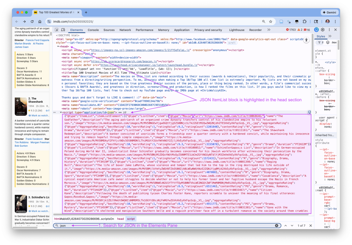
This element has HTML tag <script> with a type attribute of type="application/ld+json".
- The
<script>element does not execute JavaScript; the content is pure data intended for search engines, previews, or machine consumption. - It is usually far more stable than visible DOM text
- That is why JSON-LD is often called the “stable data layer”.
- You can see the JSON key:value pairs in the block in Figure 7.22.
The “LD” in the attribute signifies that the JSON is “Linked Data”.
- This means the content is organized based on a set of principles for publishing structured data so that:
- The data has explicit meaning (via shared vocabularies)
- Entities can be unambiguously identified
- The data can be connected (“linked”) across documents and sites
In practice, this means the data JSON-LD structure uses a well-defined schemas (most commonly from Schema.org) so the intended machine users can interpret it reliably.
This is just another type of element so we can create a CSS selector for it.
- The CSS selector combines the element HTML tag and its attribute as
'script[type="application/ld+json"]'.- Note the use of single quote on the outer edges given the double quotes in the type value.
- The selector says “Select
<script>elements where the type attribute equals application/ld+json.” - We can use this in
html_element()just like any other selector.
7.14.6.2 Extract the JSON Element
- Since we are working with JSON, load and attach the {jsonlite} package with
library(). - Open the saved file with all of the movies
- Extract the elements and extract the text from them.
# 1)
library(jsonlite)

# 2) Read the saved page (adjust path as needed)
path <- "./data/imdb_top_100_movies_live.html"
doc  <- read_html(path)

# 3) Find JSON-LD script blocks and extract their text
doc |>
  html_elements('script[type="application/ld+json"]') |>
  html_text2() ->
jsonld_txt

length(jsonld_txt)   # how many JSON-LD blocks did we find?
str_length(jsonld_txt)
class(jsonld_txt)
str_sub(jsonld_txt, 1, 150)- There is one block which is a character vector.
- But, it is a long vector as it all the embedded data for the 100 movies.
- Note: that does NOT mean it has all the data, just the data IMDb chose to expose to others in this way.
7.14.6.3 Convert from JSON and Extract a Tibble
Because this page contains a single JSON-LD block, we can parse it directly without iteration.
- Iteration is only required if we need to extract repeating items from inside the parsed object.
Here we can convert the JSON to text and examine the structure of the output.
- The first line shows there
itemListElementis a data frame. - We then see that it has two columns, one of which,
itemis a list column of the data frames. - We can use
pluck()to extract that element as save it.
The aggregateRating list column has the values for star rating and votes which are usually more precise here than in the visible DOM (for example, ratingCount is an integer rather than “2.2M”).
We can choose to unnest_wider() or just pluck().
The data frame from the JSON contains additional data and in several cases might be be easier to clean, e.g., aggregateRating-_ratingCountsince it is exact votes, not abbreviated using “M”.
- It is missing Rank but the movies are in order so we could use
- It is missing Metascore and Year which are not in the embedded data so we would have to extract and clean them from the original scraped elements.
To build the final dataset, we can treat JSON-LD as a stable “core metadata” layer and then join additional fields (metascore, year) extracted from the DOM using parent–child item scoping.
- Plot
Rankas a function ofVotes. Use a linear smoother and non-linear smoother and use a log scale on the x axis. - Interpret the plot.
- Run the linear model to check if the linear relationship is real and check the residuals with
plot().
- Since we already scraped the movie elements we do not need to rerun the live session. We can scrape from the existing
imdb_100_elemenents.
Show code
Both the linear and loess smoother show a positive relationship but the data is variable around both smoothing lines. It is not clear if the non-linear smoother is much better than the linear smoother except at the ends.
The \(p\)-value of 2.2e-16 for log(Votes) of linear model suggests there is substantial evidence of a negative relationship with rank.
However, the R-squared of .68 suggests the relationship explains a fair amount of the Star rating but it might help to add other variables.
The residual plots do not show significant issues with perhaps a slight non-linearity.
7.14.7 Example 5: Scraping Tables from Wikipedia’s Atlantic Hurricane Seasons Page
Use this example to practice:
- Extracting multiple tables
- Identifying which table(s) are relevant
- Normalizing inconsistent column sets
- Cleaning and parsing dates / numeric fields
Notes:
html_table()makes assumptions; plan for fill and post-cleaning.- Column name drift across tables is normal.
Let’s look at a Wikipedia article on hurricanes: https://en.wikipedia.org/wiki/List_of_Atlantic_hurricane_seasons
- This contains many tables which one could copy and paste into Excel but it could be a pain to clean and not amenable to being rectangular in its current form.
Let’s try to quickly get this data into tibbles using html_table().
html_table()makes a few assumptions:- No cells span multiple rows.
- Headers are in the first row.
As before, download and save the website content using read_html().
Use html_elements() to get the elements of interest, but this time we’ll extract all of the “table” elements.
- If you inspect the tables you see the name
tableand classwikitablewe can use either. Remember to add a.in front ofwikitableas a CSS class selector.
- Use
html_table()to get the tables from the table elements as a list of tibbles:
Compare the table names across the data frames.
- Use
map()to get a list where each element is a character vector of the names. - Use
map()to collapse each vector to a single string with the names separated by “:”. - Convert to a data frame for each of viewing.
7.15 Example 6: Scraping Tables of Taylor Swift Songs
Scrape the data on the Wikipedia page “List of Taylor Swift Songs” at https://en.wikipedia.org/wiki/List_of_songs_by_Taylor_Swift.
Create a line plot of the number of songs by the first year of release with a nice title, caption (the source data), and axis labels.
- Hint: Look at help for
separate_wider_delim().
- Find the CSS selector for the songs - which are in tables.
- Scrape all of the songs on the page.
- Extract as tables in a list.
- Convert only the “Released Songs” into a tibble.
- Look at the data for cleaning.
- Clean and Save
Song: remove extra"Year: Separate into two columns that are integer- Remove
Ref..
- Look at the data to check cleaning.
- Group by first year
- Summarize to get the count of the songs with
n(). - Plot with
geom_line().
Show code
swift_html_obj <- read_html("https://en.wikipedia.org/wiki/List_of_songs_by_Taylor_Swift")
xml2::write_html(swift_html_obj, "./data/swift_html_obj.html")

swift_elements <- html_elements(swift_html_obj, ".wikitable")

html_table(swift_elements)[[2]] ->
  swift_songs_df

glimpse(swift_songs_df)

swift_songs_df |>
  mutate(Song = str_replace_all(Song, '\\"', "")) |>
  separate_wider_delim(Releaseyear, delim = " and ",
                       names = c("Year_1st", "Year_2nd"),
                       too_few = "align_start") |>
  mutate(Year_1st = parse_integer(Year_1st),
         Year_2nd = parse_integer(Year_2nd)) |>
  select(-Ref.) ->
  swift_songs_df
glimpse(swift_songs_df)
Show code
swift_songs_df |>
  group_by(Year_1st) |>
  summarize(total_songs = n()) |>
ggplot(aes(Year_1st, total_songs)) +
  geom_line() +
  labs(title = "Taylor Swift Song Releases by First Year of Release",
       caption = "Source is https://en.wikipedia.org/wiki/List_of_songs_by_Taylor_Swift") +
  xlab("Year of First Release") +
  ylab("Number of Songs")
7.16 Example 7: Scrape Tables from Wikipedia Page on the Oldest Mosques
This example shows methods for integrating multiple tables with different structures and the effort required to scrape the tables and the effort it takes to clean reshape them for analysis.
The Wikipedia page on the oldest mosques in the world has tables of data about the oldest mosques in each country organized by different regions in the world.
The first step is to just look at the web page to get an idea of the data that is available and how it is organized.
- Use your browser to go to this URL: https://en.wikipedia.org/wiki/List_of_the_oldest_mosques .
We see a number of tables with different structures. However, each has data on the name of the mosque, the location country, when it was first built, and in some tables, the denomination. Many of the tables also have a heading for the region.
We want to scrape this data so we can plot the history of when were mosques first built across different regions.
- That question suggests we need to scrape the tables to get the data into a data frame suitable for plotting.
Let’s build a strategy for going from web page tables to a single data frame with tidy and clean data so we can plot.
- Inspect the web page tables.
- Use the browser’s Developer Tools to identify the right CSS selectors.
- Given the differences in the table structures we can scrape the regional information in the headers for each table separately from the tables themselves.
- Download the web page and save it as an XML object so we only have to download once. Add code to read in the XML object.
- Extract the data of interest, both headers and tables. Check we have the correct (same) number of headers and tables so we have a header for each table.
- Tidy the data into a data frame.
- Creating a data frame requires each data frame in the list to have the same variables which have the same class across the data frames.
- Clean the table headings (regions) and assign them as names for the table elements in the list of tables.
- Check the data frames for the different structures and fix any issues.
- Select the variables of interest.
- Convert into a tibble.
- Clean the data for consistent analysis.
- Ensure standard column names.
- Remove parenthetical comments.
- Convert data to be consistent of of the type desired for analysis.
We should now be able to create and interpret various plots.
7.16.1 Steps 1 and 2: Inspect Tables to Identify the CSS Selectors.
Go to this URL: https://en.wikipedia.org/wiki/List_of_the_oldest_mosques in your browser.
Look at the tables and inspect their structure/elements.
- Right-click on the table “Mentioned in the Quran” and select
Inspectto open the Developer Tools. - The Elements tab should be highlighting the element in the table where you right-clicked as in Figure 7.23.
- Move your mouse up the elements until you are highlighting the line
table class="wikitable sortable jquery-tablesorter".- You should see the table highlighted in the web page.
- The
class = "wikitable"tells us we want the CSS selector.wikitablebased onclass. - We can combine with the element html tag
tableto usetable.wikitableas a selector
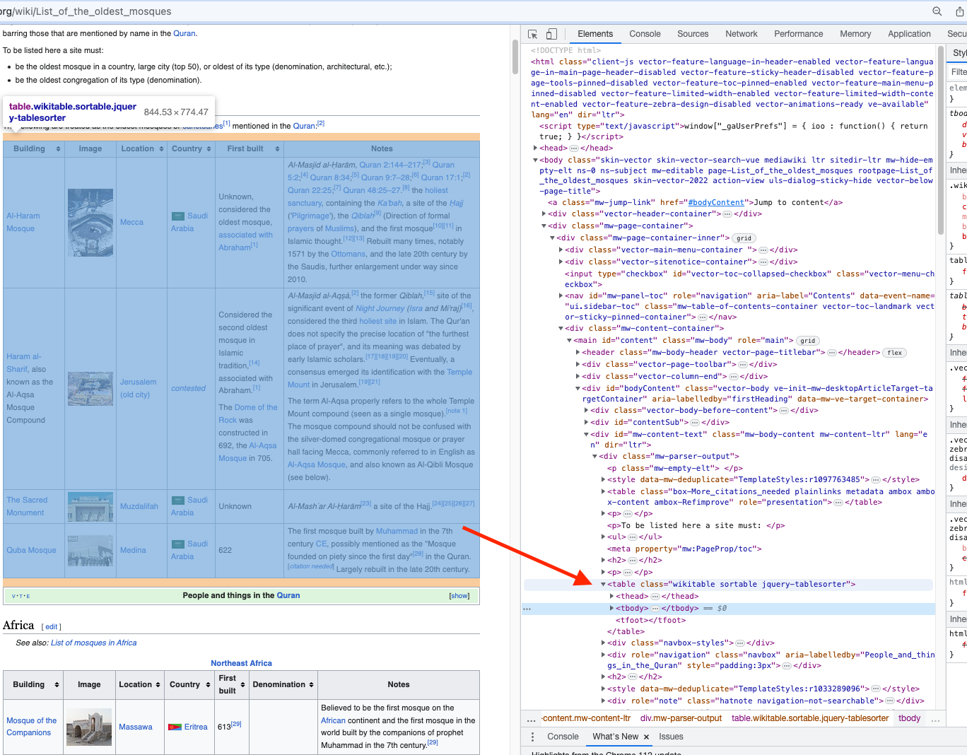
- Scroll down the elements to get to the next tag
tableso it is highlighted. Check this is alsoclass = wikitable.- You can check more tables to confirm they are all
class="wikitable"
- You can check more tables to confirm they are all
Let’s look at the regions now. These are the table headings for each region within a continent, e.g., “Northeast Africa” is a region within the continent “Africa”.
- Right-click on “Northeast Africa” and inspect it.
- It has the element
nameofcaptionso we can usecaptionas a CSS selector.- Confirm with a few other tables that the region is a
caption.
- Confirm with a few other tables that the region is a
Note that the first table, under the heading “Mentioned in the Quran” does not have a caption like the other tables.
- Right-click on “Mentioned in the Quran” and inspect it.
- It shows
id="Mentioned_in_the_Quran". Since we only want this one instance, we can use theidwith a#as a CSS selector, i.e.,#Mentioned_in_the_Quran.
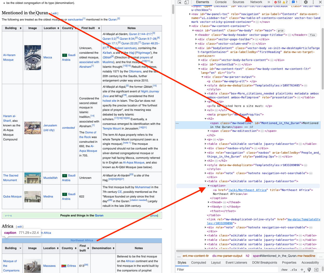
We now have selectors for each table and we can use the caption class for the regions for the tables that have them.
7.16.2 Step 3: Load (and Save) the Web Page.
Download the HTML page and save as a file.
- Then set a code chunk option
#| eval: falseso you don’t re-download each time you render and can just read in the saved file.
Read in the saved file.
- We now have the entire web page stored in an object of class
"xml-document" "xml-node".
We can now extract the elements of interest.
7.16.3 Step 4: Extract the Data of Interest
Extract the table elements and their headers (captions) using table.wikitable.
- Then extract the captions and tables them selves into a list.
- We can see from the page that not all tables have the same structure so we cannot collapse the list until we get the tables with the same columns and column types.
[1] 25List of 2
$ caption: chr NA
$ data : tibble [3 × 6] (S3: tbl_df/tbl/data.frame)
..$ Building : chr [1:3] "Al-Haram Mosque" "Al-Aqsa Mosque Compound (Al-Aqsa)" "Quba Mosque"
..$ Image : logi [1:3] NA NA NA
..$ Location : chr [1:3] "Mecca" "East Jerusalem" "Medina"
..$ Country : chr [1:3] "Saudi Arabia" "Administered by Israel, part of occupied Palestine" "Saudi Arabia"
..$ First built: chr [1:3] "Unknown, considered the oldest mosque, associated with Abraham[1]" "Considered the second oldest mosque in Islamic tradition,[14] associated with Abraham.[1]First prayer hall buil"| __truncated__ "622"
..$ Notes : chr [1:3] "Al-Masjid al-Ḥarām,[a] the holiest sanctuary, containing the Ka'bah, a site of the Ḥajj ('Pilgrimage'), the Qib"| __truncated__ "Al-Masjid al-Aqṣá,[2] the former Qiblah,[15] site of the significant event of Night Journey (Isra and Mi'raj)[1"| __truncated__ "The first mosque built by Muhammad in the 7th century CE, mentioned as the \"Mosque founded on piety since the "| __truncated__List of 2
$ caption: chr "Northeast Africa"
$ data : tibble [6 × 7] (S3: tbl_df/tbl/data.frame)
..$ Building : chr [1:6] "Mosque of the Companions" "Al Nejashi Mosque" "Mosque of Amr ibn al-As" "Mosque of Ibn Tulun" ...
..$ Image : logi [1:6] NA NA NA NA NA NA
..$ Location : chr [1:6] "Massawa" "Negash" "Cairo" "Cairo" ...
..$ Country : chr [1:6] "Eritrea" "Ethiopia" "Egypt" "Egypt" ...
..$ First built: chr [1:6] "620s–630s" "7th century" "641" "879" ...
..$ Tradition : chr [1:6] "" "" "" "" ...
..$ Notes : chr [1:6] "Believed by some to be the first mosque in Africa and built by the companions of Muhammad in the 7th century.[25]" "By tradition, the burial site of several followers of Muhammad who, during his lifetime, fled to the Aksumite K"| __truncated__ "Named after 'Amr ibn al-'As, commander of the Muslim conquest of Egypt. First mosque in Egypt and claimed to be"| __truncated__ "" ...- We now have 25 tables in a list where each elements is a list of 2 with the first element of a character and the second element is a tibble with the data.
The first table has NA for the caption so we can add it now using the id selector (which has a unique value).
List of 2
 $ caption: chr "Mentioned in the Quran"
 $ data   : tibble [3 × 6] (S3: tbl_df/tbl/data.frame)
  ..$ Building   : chr [1:3] "Al-Haram Mosque" "Al-Aqsa Mosque Compound (Al-Aqsa)" "Quba Mosque"
  ..$ Image      : logi [1:3] NA NA NA
  ..$ Location   : chr [1:3] "Mecca" "East Jerusalem" "Medina"
  ..$ Country    : chr [1:3] "Saudi Arabia" "Administered by Israel, part of occupied Palestine" "Saudi Arabia"
  ..$ First built: chr [1:3] "Unknown, considered the oldest mosque, associated with Abraham[1]" "Considered the second oldest mosque in Islamic tradition,[14] associated with Abraham.[1]First prayer hall buil"| __truncated__ "622"
  ..$ Notes      : chr [1:3] "Al-Masjid al-Ḥarām,[a] the holiest sanctuary, containing the Ka'bah, a site of the Ḥajj ('Pilgrimage'), the Qib"| __truncated__ "Al-Masjid al-Aqṣá,[2] the former Qiblah,[15] site of the significant event of Night Journey (Isra and Mi'raj)[1"| __truncated__ "The first mosque built by Muhammad in the 7th century CE, mentioned as the \"Mosque founded on piety since the "| __truncated__
We are finished scraping so are ready to clean and tidy the data for analysis.
7.16.4 Step 5: Tidy the data
Use {purrr} and other functions to convert the list of tables to a tidy tibble.
7.16.4.1 Clean the captions and assign to the list.
Cleaning the captions and adding them as names for the data frame elements in the list will make our data easier to look at.
Look at the captions for cleaning ideas.
 [1] "Mentioned in the Quran"
 [2] "Northeast Africa"
 [3] "Northwest Africa"
 [4] "Southeast Africa (including nearby islands of the Indian Ocean, but barring countries that are also in Southern Africa)"
 [5] "Southern Africa"
 [6] "West Africa"
 [7] "Arabian Peninsula (including the island-state of Bahrain)"
 [8] "Levant (including Cyprus and the region of Syria)"
 [9] "West Asia (excluding the Arabian peninsula, Caucasus, and Levant)"
[10] "Transcaucasia (excluding the Russian North Caucasus)"
[11] "Central Asia"
[12] "Greater China"
[13] "South Asia"
[14] "Southeast Asia"
[15] "East Asia (excluding Greater China)"
[16] "Central Europe and Eastern Europe (excluding the Caucasus, European Russia and Nordic countries)"
[17] "Iberian Peninsula"
[18] " Russia"
[19] "Scandinavia"
[20] "United Kingdom and Ireland"
[21] "Western-Central Europe (excluding the British Isles, Nordic countries, and countries that are also in Eastern Europe)"
[22] "North America (including Central America and island-states of the Caribbean Sea)"
[23] "South America"
[24] "Australasia"
[25] "Melanesia" - Several have parenthetical phrases we don’t need.
- ” Russia” has a leading space for some reason.
Let’s use {stringr} and regex to get rid of the extra text.
map_chr(mosque_tables, "caption") |>
  str_remove_all("\\s*\\([^)]*\\)") |> # drop parenthetical notes
  str_remove_all("\\[[0-9]+\\]") |> # drop footnote markers like [12] if present
  str_squish() |>
  make.unique() -> # be safe and ensure names are unique
cap_names

names(mosque_tables) <- cap_names # Assign as names

str(mosque_tables, max.level = 2)
List of 25
$ Mentioned in the Quran :List of 2
..$ caption: chr "Mentioned in the Quran"
..$ data : tibble [3 × 6] (S3: tbl_df/tbl/data.frame)
$ Northeast Africa :List of 2
..$ caption: chr "Northeast Africa"
..$ data : tibble [6 × 7] (S3: tbl_df/tbl/data.frame)
$ Northwest Africa :List of 2
..$ caption: chr "Northwest Africa"
..$ data : tibble [11 × 7] (S3: tbl_df/tbl/data.frame)
$ Southeast Africa :List of 2
..$ caption: chr "Southeast Africa (including nearby islands of the Indian Ocean, but barring countries that are also in Southern Africa)"
..$ data : tibble [7 × 7] (S3: tbl_df/tbl/data.frame)
$ Southern Africa :List of 2
..$ caption: chr "Southern Africa"
..$ data : tibble [8 × 7] (S3: tbl_df/tbl/data.frame)
$ West Africa :List of 2
..$ caption: chr "West Africa"
..$ data : tibble [6 × 7] (S3: tbl_df/tbl/data.frame)
$ Arabian Peninsula :List of 2
..$ caption: chr "Arabian Peninsula (including the island-state of Bahrain)"
..$ data : tibble [11 × 7] (S3: tbl_df/tbl/data.frame)
$ Levant :List of 2
..$ caption: chr "Levant (including Cyprus and the region of Syria)"
..$ data : tibble [11 × 7] (S3: tbl_df/tbl/data.frame)
$ West Asia :List of 2
..$ caption: chr "West Asia (excluding the Arabian peninsula, Caucasus, and Levant)"
..$ data : tibble [14 × 7] (S3: tbl_df/tbl/data.frame)
$ Transcaucasia :List of 2
..$ caption: chr "Transcaucasia (excluding the Russian North Caucasus)"
..$ data : tibble [2 × 7] (S3: tbl_df/tbl/data.frame)
$ Central Asia :List of 2
..$ caption: chr "Central Asia"
..$ data : tibble [1 × 7] (S3: tbl_df/tbl/data.frame)
$ Greater China :List of 2
..$ caption: chr "Greater China"
..$ data : tibble [11 × 7] (S3: tbl_df/tbl/data.frame)
$ South Asia :List of 2
..$ caption: chr "South Asia"
..$ data : tibble [13 × 7] (S3: tbl_df/tbl/data.frame)
$ Southeast Asia :List of 2
..$ caption: chr "Southeast Asia"
..$ data : tibble [8 × 7] (S3: tbl_df/tbl/data.frame)
$ East Asia :List of 2
..$ caption: chr "East Asia (excluding Greater China)"
..$ data : tibble [2 × 7] (S3: tbl_df/tbl/data.frame)
$ Central Europe and Eastern Europe:List of 2
..$ caption: chr "Central Europe and Eastern Europe (excluding the Caucasus, European Russia and Nordic countries)"
..$ data : tibble [19 × 7] (S3: tbl_df/tbl/data.frame)
$ Iberian Peninsula :List of 2
..$ caption: chr "Iberian Peninsula"
..$ data : tibble [11 × 7] (S3: tbl_df/tbl/data.frame)
$ Russia :List of 2
..$ caption: chr " Russia"
..$ data : tibble [4 × 6] (S3: tbl_df/tbl/data.frame)
$ Scandinavia :List of 2
..$ caption: chr "Scandinavia"
..$ data : tibble [6 × 7] (S3: tbl_df/tbl/data.frame)
$ United Kingdom and Ireland :List of 2
..$ caption: chr "United Kingdom and Ireland"
..$ data : tibble [2 × 7] (S3: tbl_df/tbl/data.frame)
$ Western-Central Europe :List of 2
..$ caption: chr "Western-Central Europe (excluding the British Isles, Nordic countries, and countries that are also in Eastern Europe)"
..$ data : tibble [5 × 7] (S3: tbl_df/tbl/data.frame)
$ North America :List of 2
..$ caption: chr "North America (including Central America and island-states of the Caribbean Sea)"
..$ data : tibble [11 × 7] (S3: tbl_df/tbl/data.frame)
$ South America :List of 2
..$ caption: chr "South America"
..$ data : tibble [7 × 7] (S3: tbl_df/tbl/data.frame)
$ Australasia :List of 2
..$ caption: chr "Australasia"
..$ data : tibble [3 × 7] (S3: tbl_df/tbl/data.frame)
$ Melanesia :List of 2
..$ caption: chr "Melanesia"
..$ data : tibble [3 × 7] (S3: tbl_df/tbl/data.frame)- We can see the elements are now named. We can also see that they have different numbers of rows which is fine, but at least one has a different numbers of columns which needs to be adjusted.
7.16.4.2 Convert the Data into a Tidy Data Frame.
We want to turn the list into a single tibble so we have to ensure each tibble shares the same column names and consistent classes..
Let’s look at the column names and classes for each tibble in the list.
Let’s use purrr::imap() to operate on the list elements using their names as the index.
imap_*()functions are versions ofmap2_*()functions where the second argument comes from an index associated with the data.- If the input is a named vector/list, the index uses the name of each element, else the numeric index.
- This allows us to access to the elements within each list element that gets passed by
imap().
- We are interested in the tibbles so using
map_chr()withclasswill return a named vector with the column names and classes.
For simplicity, lets use visual inspection of the results to check for consistency of column names and classes across the tibbles.
- If we had many more lines, we could convert each tibble’s results to a tibble (with columns for the
Region = region,variable = names(x$data), andclass = map_chr(x$data, class)), uselist_rbind()andpivot_wider(), and then summarize withn_distinct()to find values > 1.
Looking at all of the elements, we can see several issues with the columns
- The first element (“Mentioned in the Quran”) is missing a column for
Tradition, - Elements “Levant” and “Central Europe and Eastern Europe” use column name
Built(CE)instead ofFirst built, and, - Element Russia” is missing
Country. - Looking closely at
First builtandBuilt(CE)different tibbles have different classes. - The same is true for true for
Traditionas missing values are assigned logical instead of character.
We have to do some initial cleaning so we can tidy the data.
- Add a column for
Traditionto the first element’s tibble. - Standardize name
First builttoFirst_Builtand convertBuilt(CE)toFirst_Builtwhere it exists across all tibbles. - Add a column
Countryto element “Russia” tibble. - Let’s convert everything to character to ensure consistency and we can fix classes after creating the single tibble.
Since we want to access both the caption and data elements, let’s use imap() to operate on the list elements using their names as the index.
- We can access each element in the
imapexpression as needed to make fixes. - Saving the result with a different variable name eases troubleshooting.
imap(mosque_tables, \(x, region) {
  # 1) Use the list element names we created from the captions as region.)
  x$caption <- region

  # 2) Grab the tibble
  df <- x$data

  # 3) Ensure Tradition exists
  if (!"Tradition" %in% names(df)) {
    df <- df |> mutate(Tradition = NA_character_)
  }

  # 4) Standardize column names we want (Only rename if the old name exists.)
  if ("First built" %in% names(df)) {
    df <- df |>
      rename(First_Built = `First built`)
  } else if ("Built(CE)" %in% names(df)) {
    df <- df |>
      rename(First_Built = `Built(CE)`)
  }

  # 5) Add Country column  to Russia
  if (region == "Russia") {
    df <- df |>
      mutate(Country = "Russia", .after = Location)
  }

  # 6) Convert all columns to character to be predictable (often worth it for Wikipedia)
  df <- df |>
    mutate(across(everything(), as.character))

  # 7) Save the updated df
  x$data <- df

  x
}) -> mosque_tables_c

# quick sanity check
str(mosque_tables_c[[1]], max.level = 1)
glimpse(mosque_tables_c[[1]]$data)
glimpse(mosque_tables_c[["Levant"]]$data)
glimpse(mosque_tables_c[["Russia"]]$data)
Now that we have the same column names and classes for each data frame, we can convert the list to a tibble.
Let’s use imap() to extract the data frames as a list and then use list_rbind with the names_to = argument to keep the element names as a new column.
Our data of interest is now in a tidy data frame with 184 rows and 8 columns.
It is time to look at the data to see what cleaning needs to be done.
7.16.5 Step 6 : Clean the Data.
You can view() the data frame to look for cleaning opportunities.
We already know there are issues with First_Built since we could see different classes earlier.
First_Builtvalues are a mix of text, dates as centuries, and dates as years.- There are multiple footnotes demarcated by
[]which we do not need. - Let’s replace century dates with the last year of the century, e.g., “15th” becomes “1500”.
- We can then extract any set of numbers with at least three digits which means we don’t have to worry about the footnotes.
Several of the country names have parenthetical comments. Let’s remove those.
- The regex is designed to be safe by only removing text within a single set of parentheses by stopping matching at the first closing parenthesis.
- Note the
)does not need to be escaped when it is inside the[]where it is not treated as a special character.
We now have a tidy data frame with cleaned data for analysis
There are no hard and fast rules for the choices you will make in cleaning other than to get the data in a state that is useful for analysis.
In this example, you could try to find missing dates in other sources but for now we will let them stay as missing.
7.16.5.1 Plotting the Data.
Let’s plot the building of the mosques over time by region.
- Reorder the regions based on the earliest data a mosque was first built
- Make the title dynamic based on the number of mosques actually used in the plot.
- Use the magrittr pipe
%>%with theggplot()call embraced with{}so you can refer to the data frame with.
- Use the magrittr pipe
mosque_df_c |>
  filter(!is.na(Region), !is.na(First_Built)) %>%
  {ggplot(., aes( x = fct_reorder(.f = Region, .x = First_Built, .fun = min,
      na.rm = TRUE ),
    y = First_Built )) +
  geom_point(alpha = .5) +
  coord_flip() +
  labs(
    x = "Region", y = "First Built",
    title = glue::glue("First Built Dates for { nrow(.) } Prominent Mosques by Region"),
    subtitle = "Does not include mosques whose built date is unknown.",
    caption = "Source- Wikipedia"
)}Create a bar plot of the number of oldest mosques by Country for those countries with more than one oldest mosque.
- Group by country
- Mutate to add the count of mosques to the data frame
- Ungroup
- Filter to countries with more than one mosque
- Plot
- Reorder the countries by count
- Rotate the X axis titles by 90 degrees.
- Add Title, Caption, and X axis label.
Show code
mosque_df |>
  group_by(Country) |>
  mutate(count = n()) |>
  ungroup() |>
  filter(count > 1) |>
ggplot(aes(x = fct_reorder(Country, .x = count) )) +
  geom_bar() +
  theme(axis.text.x = element_text(angle = 90, vjust = 0.5, hjust = 1)) +
  xlab("Country") +
  labs(title = "Countries with Two or More of the Oldest Mosques",
       caption = "source = Wikipedia https://en.wikipedia.org/wiki/List_of_the_oldest_mosques")
7.17 Common Debugging Patterns
When something fails, identify which pipeline stage failed.
- Request failure: status code, blocking, rate limiting
- Response mismatch: consent or bot page
- Parse mismatch: wrong object type or empty nodes
- Extraction mismatch: selector too broad or too narrow
- Normalization mismatch: alignment issues due to missing fields
- Cleaning mismatch: parsing assumptions not met
A disciplined approach is:
- Inspect small samples.
- Check counts at every stage.
- Build a minimal working extractor before scaling up.
7.18 “Oh, By the Way, This Transfers to Python”
Everything in this chapter is a language-independent model.
The pipeline is the same:
- Request
- Response
- Parse
- Extract
- Normalize and align
- Clean and validate
Python uses different tools, but the same decisions and failure modes apply.
7.18.1 Concept Mapping (R ↔︎ Python)
- HTTP requests
- R:
read_html(),httr::GET() - Python:
requests.get()
- R:
- User-Agent and headers
- R:
httr::user_agent(),httr::add_headers() - Python:
headers={...}inrequests.get()
- R:
- Parsed document tree
- R: {xml2} document, nodes, node sets
- Python: Beautiful Soup (
bs4) parse tree, orlxmlelement tree
- Selection
- R:
html_element(),html_elements()withcss=orxpath= - Python:
.select_one(),.select()(CSS), or XPath vialxml
- R:
- Text and attributes
- R:
html_text2(),html_attr() - Python:
.get_text(),tag.get("href")
- R:
- Embedded JSON
- R:
jsonlite::fromJSON() - Python:
json.loads()
- R:
- Dynamic pages (rendered DOM)
- R:
read_html_live(), {chromote} - Python: Selenium or Playwright
- R:
The key takeaway:
- The hard part is not the language.
- The hard part is identifying the correct data layer and building a robust, validated extraction pipeline.
7.19 Scraping Multiple (Dynamic) Web Pages
Two common use cases involve scraping multiple web pages.
One use case is scraping the results on one page to get URLs you can use to scrape other pages.
- In the simplest version, the webpage is static so the URLs for the other pages are visible in the DOM.
- One can combine functions from the {rvest} package and the {purrr} package to scrape multiple pages automatically and get the results into a single tibble.
- The goal is to create a tibble with variables page ID, URL, and CSS selectors and then add columns with the scraped elements of interest and the scraped text as a column of tibbles.
- This way, all the data is in one object which documents how the data was collected in addition to the data and it can be stored for later analyses.
A second use case is when a website has content that is long to be displayed on a single page.
- A common method is to use multiple pages that adjust the content between pages dynamically as the size of viewport changes depending upon the device and zoom level.
- This is more complicated as it requires working with dynamic web pages.
7.19.1 Dynamic Web Pages, Asynchronous Coding, and Promises
When a web page is dynamic, it uses javascript to either load additional elements on the page as you scroll or control what happens when you click on the page.
The {rvest} package works well on static HTML and with its live capabilities can work with some package actions, however it can be insufficient to get the information you need on highly dynamic pages.
You need packages that support interacting with the website in a code-driven manner. These are typically packages based on frameworks for testing web sites using test scripts.
The developer writes the scripts and the package uses a “headless” browser (one not visible in the browser) to execute actions such as scrolling and clicking on the page to see if the web site behaves as intended.
Playwright is a relatively new capability for script-driven web site testing developed by Microsoft. It uses the node.js framework for javascript and fits works well with python.
The {rplaywright} package is a recent package that provides a wrapper around Playwright.
Many websites are developed using an asynchronous approach to coding.
In a synchronous approach, each operation (function) has to complete and return a result before starting the next operation, e.g., each step in a piped process must deliver the results before the next step can start.
In an asynchronous approach, the code can start a process but does not need to wait for it to finish before starting another process that does not depend on the results from the first process. This is especially useful in situations such as a website where multiple users may want to run processes at the same time and don’t want to wait for another user’s process to finish.
The javascript community refers to the asynchronous processes as creating a “promise” object which links the initiated code (the producing code) to the code that is waiting to work with the results (the consuming code).
When working with asynchronous code, the “promise” object is not the same as the “promise” object one gets as part of base R lazy evaluation. Both are approaches to deferred results, but their structures are completely different.
The {promises} package “brings asynchronous programming capabilities to R.” It is most useful when designing deployed applications e.g., shiny, where you want to support multiple users at once and some operations take a long time. Those are the ones you want to make asynchronous.
As the vignettes make clear, working with asynchronous programming is complicated as is not used for most R projects. Read the vignettes carefully.
7.19.2 Inspecting India Today Pages to Limit What Gets Scraped.
India Today is a media conglomerate whose elements include news, magazines and other media.
Its website provides a good refresher in identifying the css elements to focus the scraping to the items of interest and reduce clutter from similar elements that are not of interest.
- We are interested in scraping a single page which has information about each state and union territory in India: https://www.indiatoday.in/education-today/gk-current-affairs/story/list-of-indian-states-union-territories-with-capitals-1346483-2018-09-22.
- The data of interest is in the middle of the page and we don’t want all the extra material on the page.
A few tries with SelectorGadget gets to selector .paywall :nth-child(1).
- This yields one big blob of text plus redundant text that will take a lot of cleaning (
india_1below). - Using the browser Inspect tool shows
h3for the state names andlifor the list items. Using them alone captures extra elements outside the center of the page (india_2below). - The Inspect tool shows other classes such as
main__contentordescriptionthat only include elements in the center section.
- Add in the parent div with class
descriptionwill limit toh3andlithat are within thedescriptionclass div to reduce the extra scraped items (india_3below). This still includes one introductory paragraph not of interest. - Finally, you can use the inspect tool to get very specific on classes for the items of interest and select only them (
india_4below).
[1] 153[1] 295[1] 132[1] 131Each of the option returns character vectors of different lengths
You can see some of the differences by creating a tibble with a list column unnesting it, selecting just the first 10 columns, and shortening their contents.
# A tibble: 4 × 5
  option `data-1`               `data-2`               `data-3`         `data-4`
   <dbl> <chr>                  <chr>                  <chr>            <chr>
1      1 "India, a union of st" "India, a union of st" "There are 29 s… adverti…
2      2 "India Today"          "Aaj Tak"              "India Today Hi… NewsTak
3      3 "Let's take a look at" "1. Andhra Pradesh - " "Hyderabad was … The Bud…
4      4 "1. Andhra Pradesh - " "Hyderabad was the fo" "The Buddhist S… Recogni…
This example shows there are often multiple ways to scrape a page to balance the level of effort in scraping versus cleaning the data.
It also demonstrates the value of using the browser Inspect tool to get a broader perspective of the page structure.
These notes and examples just touch the surface of creating better CSS selectors.
Use the developer tools to inspect the page and then explore various options for selectors to scrape the text you want and only the text you want.
7.19.3 Scraping Dynamic Pages on Vikaspedia
Vikaspedia is a multi-language information portal sponsored by the government of India.
- We are interested in scraping the data about e-government initiatives in each state that is listed on https://vikaspedia.in/e-governance/states.
- This page lists each state and one can link to a page with a list of the e-government initiatives in the state and some short information about the initiatives.
- When you go to a state page, the data of interest is in the middle column of the page and we don’t want any of the comments and extra material, e.g., as seen on the sides of the page at https://vikaspedia.in/e-governance/states/andhra-pradesh.
Although the page layouts for the India today and Vikaspedia sites are similar in that we eventually want the data in the middle of the page, the pages come from different sites so the DOM and CSS structure is quite different between them.
7.19.3.1 Scraping Strategy
There are 31 states in India. Instead of manually getting their URLs and scraping each page individually, we want to develop code to scrape the overarching page with all the states and build a data frame of the individual state pages to scrape with their URLs. This assumes that each state page shares a common DOM and CSS structure.
This strategy allows us to adjust the tibble contents as appropriate as the analysis needs change or the web pages change over time.
This use case is an example of a strategy template where you have a set of data you want to use as arguments to a function.
- In this example, we have a set of many URLs we want to use as arguments to functions.
For these kinds of use cases, you could use a spreadsheet file to manage the arguments data over time instead of embedding it in your code. You could also add the CSS selectors into the spreadsheet.
Since it is now data, not code, It is easier to collaborate and configuration manage the data in a shared spreadsheet file than in R code (especially with people not on GitHub).
- You can adjust the code to use the {readxl} or {googlesheets4} package to read in the data, or,
- Export a .csv file to a data_raw directory and use
readr::read_csv()and a relative path to load the data into a tibble.
A similar use case is where humans generate free text data for fields, such as business names, where there is a “canonical” or standard name in the analysis so all data aligns to the correct name, but the humans tend to be overly creative and make their own variants of the names.
- Say the canonical name is “First Union Bank”. Humans might use “1st Union Bank” or “First Union Bk”.
Instead of trying to use Regex to manage all the variants, create a spreadsheet with the standard names in one column and all the erroneous variants you have had to fix in the second.
- Read in the spreadsheet and use it to clean the data using a join.
- You can also have the code identify any “new” errors which you can then add to the spreadsheet once you figure out what the correct standard is.
While you might think you can impose a standard on humans, if you don’t have a drop-down form with the canonical names so they are entering in free text, it is more robust to manage on the back end as data and outside of your code.
7.19.3.2 Step 1: Inspect the Page
If we go to the all states page https://vikaspedia.in/e-governance/states, we see some of the states.
The presence of multiple pages (depending upon your initial viewpoint size) indicates that this is a dynamic page and if we want all the states we will have to get the code to “click” on the next page.
Each page used to be a static page where the 30 states were on the first page were all loaded with the page and the unique portion of each state URL was visible on the page. - That portion could be combined with the canonical link for the site to create each state’s unique URL.
However the page has been restructured to be dynamic and javascript-driven.
- The number of states that load on the first page depends upon the size of the initial viewport.
- Smaller viewports mean fewer states per page and more pages to scrape.
- This is determined dynamically when the page is first opened.
- The State URLs are no longer visible at all.
- The URL is retrieved by by a javascript call to an API when the state is clicked on.
- If you use the Browser inspect tool and look at the Network Tab you can see the call happen when you click on an individual state.
Using the inspect tool
- The state elements are within a central div container with class
div.MuiGrid-root.MuiGrid-container.MuiGrid-spacing-xs-2.mui-isbt42. - Drilling down into a state div we can find a state element with name
h6which has the “title” attribute of the state name.
However the URL is not.
- One could use a dynamic tool to use javascript to capture the eventual URL based on “clicking” each state and tracking the API call. This can be quite complicated.
- However, in this example, clicking on several states and checking their URLs shows what appears to be a simple pattern.
- Take the state name, convert to lower class. If the name has more than one word in it, replace any characters between the words with a
-. - We will use that strategy to create the URLs for each state.
Thus to get the state names and URLs we will use the {rplaywright} package for interacting (and scraping) dynamic web sites.
7.19.3.3 Step 1a: Install {rplaywright}, Playright, and Node.js
Use the console to install {rplaywright} from GitHub with devtools::install_github("erikaris/rplaywright").
The {rplaywright} package is relatively new and has limited support, limited users, and only one minimalist vignette.
- It does work but can be complicated as it has some limitations that are not present in the python implementation of Playwright.
- LLMs still struggle with getting it right.
If you have serious scraping to do and want to use Playwright, using python might be an easier path.
If working in R, go through the vignettes for the {promises} package to get helpful background for understanding the R approach to Javascript promises used in {rplaywright}.
The {rplaywright} package is a wrapper for the Playwright Node.js library. so you need to have that installed on your system as well.
- For Macs: - use Homebrew with
brew install nodein the terminal. - For windows: Download installer from the Node.js organiztion.
Once installed, Check the versions using the terminal with node --version and npm --version. Both should return a version number. As of April 2025 that should be at least v23.11.0 and 10.9.2.
Then use the terminal to install the playwright software with npx playwright install.
7.19.3.4 Step 2. Create the Tibble of State Names and URLs from the All States Page
Given what we have learned from inspecting the page, we want to create a script to extract individual state names and create the URLs from the given all states page URL.
We will start with creating a script to scrape one page, regardless of how many states are on it.
You will notice several lines of code, e.g., to browser$new_context()$then(), that use the then() function.
- This code is asynchronous. The first part (
browser$new_context()) is generating a js promise and thethen()is acting on the promise to generate the results of the first promise. - One of the challenges is that the
then()function as implemented in {rplaywright} appears to return another promise (the expected behavior) for most calls but in some cases, e.g.,page$content()$then(), whenthen()has no arguments, it returns the value.
The following script goes through several steps.
- Initialize the browser, set the context and open a default page. Each of these are promises.
- Navigate to the URL for the all states page. Sleep for a few seconds to allow the page to load.
- Get the entire page’s HTML as a character variable.
- Close the browser and stop chromium.
Now the rest is regular R code.
- Parse the HTML to recreate the hierarchical structure of the DOM and CSS elements so they can be extracted.
- Extract the elements of interest to get to the state names as a vector.
- Create the function to generate URL slugs
- Create the tibble with the state names and URLs
library(rplaywright)
library(rvest)
library(dplyr)
library(stringr)
library(purrr)
library(logger)

# turn off logging completely
log_threshold(TRACE)   # sets the lowest level
log_appender()  # drop all output

# 1 Initialize Playwright
browser <- rplaywright::new_chromium()
context <- browser$new_context()$then()
page <- context$new_page()$then()

# 2 Navigate to the page
page$goto("https://en.vikaspedia.in/viewcontent/e-governance/states")$then()

# Use Sys.sleep
Sys.sleep(6)  # Wait 6 seconds for the page to fully load

# 3 Get the current page HTML
html_content <- page$content()$then()

# 4 Close the browser and stop the underlying chromium process when done
browser$close()$then()
stop_server()


# 5 Parse the HTML with rvest as usual
parsed_html <- read_html(html_content)

# 6 Extract state information using rvest getting the outer elements and
# then the inner elements
css_state_container <- "div.MuiGrid-root.MuiGrid-container.MuiGrid-spacing-xs-2.mui-isbt42"
css_state_item <- "h6"

state_elements <- parsed_html  |>
  html_element(css_state_container)  |>
  html_elements(css_state_item)

# Extract state names from the elements
state_names <- state_elements %>%
  html_text()  |>
  trimws() # remove leading training white spaces

# 7 Create a generate_slug function to create the URL slug for a state name
generate_slug <- function(state_name) {
  state_name %>%
    str_to_lower()  |>
    str_replace_all("&", "and") |>
    str_replace_all(" ", "-")  |>
    str_remove_all("[^a-z0-9-]")
}

# 8 Create a tibble with state information and URLs
state_df <- tibble(
  state_name = state_names
)  |>
  mutate(
    # Generate URL slug from state name using purrr
    url_slug = map_chr(state_name, generate_slug),
    # Construct full URL
    url = str_c("https://en.vikaspedia.in/viewcontent/e-governance/states/",
                url_slug, "?lgn=en")
  )
The above code returns a data frame with 12 states as that is how many appeared in the viewport for the default headless browser.
Now that we can get the data from one page. Let’s turn the extraction from a page into a function and use that and the slug function as part of a loop to go through each page.
- This is an example where a for-loop is helpful as we do not know how many pages we will need to process.
Let’s convert the script code into a function that takes the rplaywright page object as an argument and returns a data frame.
#' Extract state information from a single page
#'
#' @param page A rplaywright page object
#' @return A data frame containing state names and their URLs

library(rplaywright)
library(rvest)
library(dplyr)
library(purrr)

extract_states_from_page <- function(page) {
  # Get the current page HTML
  html_content <- page$content()$then()

  # Parse the HTML with rvest
  parsed_html <- read_html(html_content)

  # Extract state information using rvest
  state_elements <- parsed_html  |>
    html_element(css_state_container)  |>
    html_elements(css_state_item)

  # Extract state names from the elements
  state_names <- state_elements  |>
    html_text()  |>
    trimws()

  # If no states found, return empty data frame
  if (length(state_names) == 0) {
    return(data.frame())
  }

  # Create a data frame with state information and URLs
  state_df <- data.frame(
    state_name = state_names,
    stringsAsFactors = FALSE
  )  |>
    mutate(
      # Generate URL slug from state name
      url_slug = map_chr(state_name, generate_slug),
      # Construct full URL
      url = str_c("https://en.vikaspedia.in/viewcontent/e-governance/states/",
                  url_slug, "?lgn=en")
    )
  return(state_df)
}
The generate_slug() function.
Now use these functions to go through each page.
You will see javascript (from Claude) in the code below to find and select the buttons.
- While {rplaywright} has a function to click buttons, in this example which uses Material UI (MuiPagination) framework, the page buttons are dynamic themselves.
- There can be different numbers of buttons based on how the initial viewport is set with fewer pages for larger viewports.
- This makes it much more complicated to find and select them.
- Thus the javascript approach is considered more robust.
This function goes through several steps
- Initialize the playwright objects
- Go to the initial page and wait for it to load.
- Extract the states from the first page using the defined function.
- Determine the number of pages
- Find all the buttons for the pages.
- Use a for-loop to go through the remaining pages.
- Extract the states from each page and add to the data frame.
- Close the browser and stop chromium.
#' Scrape all state information from multiple pages
#'
#' @param base_url The base URL to start scraping from
#' @return A data frame containing all state names and their URLs across all pages
#'
library(rplaywright)
library(rvest)
library(dplyr)
library(purrr)

scrape_all_states <- function(base_url = "https://en.vikaspedia.in/viewcontent/e-governance/states") {
  # 1. Initialize Playwright
  browser <- rplaywright::new_chromium()
  context <- browser$new_context()$then()
  page <- context$new_page()$then()

  # 2 Navigate to the initial page
  page$goto(base_url)$then()

  # Wait for the page to load
  Sys.sleep(6)

  # 3 Extract states from the first page
  all_states <- extract_states_from_page(page)

  # 4 Get total number of pages
  html_content <- page$content()$then()
  parsed_html <- read_html(html_content)

  # 5 Extract page buttons (excluding first/last and prev/next buttons)
  page_buttons <- parsed_html %>%
    html_elements(".MuiPagination-ul li button.MuiPaginationItem-page") %>%
    html_text() %>%
    as.numeric()

  total_pages <- if (length(page_buttons) > 0) max(page_buttons) else 1

  # 6 Process remaining pages
  if (total_pages > 1) {
    for (page_num in 2:total_pages) {
      cat("Processing page", page_num, "of", total_pages, "\n")

      # Find and click the button for the current page number
      js_code <- paste0("
        () => {
          const pageButtons = Array.from(document.querySelectorAll('.MuiPagination-ul li button.MuiPaginationItem-page'));
          const targetButton = pageButtons.find(button => button.textContent.trim() === '", page_num, "');
          if (targetButton) {
            targetButton.click();
            return true;
          }
          return false;
        }
      ")

      button_clicked <- page$evaluate(js_code)$then()

      if (!button_clicked) {
        # Try clicking the next button as a fallback
        next_button_js <- "
          () => {
            const nextButton = document.querySelector('button[aria-label=\"Go to next page\"]');
            if (nextButton) {
              nextButton.click();
              return true;
            }
            return false;
          }
        "
        button_clicked <- page$evaluate(next_button_js)$then()

        if (!button_clicked) {
          warning("Could not navigate to page ", page_num)
          break
        }
      }

      # Wait for page to load
      Sys.sleep(2)

      # 7 Extract states from the current page
      current_page_states <- extract_states_from_page(page)

      # Append to the full dataset
      all_states <- bind_rows(all_states, current_page_states)
    }
  }

  # 8 Close the browser
  browser$close()$then()
  stop_server()

  # Return the complete dataset
  return(all_states)
}
Now that all the functions are set up, lets get all the states’ data.
# A tibble: 6 × 3
  state_name    url_slug      url
  <chr>         <chr>         <chr>
1 Tamil Nadu    tamil-nadu    https://en.vikaspedia.in/viewcontent/e-governance…
2 Tripura       tripura       https://en.vikaspedia.in/viewcontent/e-governance…
3 Uttar Pradesh uttar-pradesh https://en.vikaspedia.in/viewcontent/e-governance…
4 Uttarakhand   uttarakhand   https://en.vikaspedia.in/viewcontent/e-governance…
5 West Bengal   west-bengal   https://en.vikaspedia.in/viewcontent/e-governance…
6 Telangana     telangana     https://en.vikaspedia.in/viewcontent/e-governance…
We now have a data frame of all 31 state names and URLs.
7.19.3.5 Step 3. Use the Tibble of State Names and URLs to Scrape each States Page.
Using the browser tools to inspect the pages for the states shows that the content of interest is in the middle in the div with id=MiddleColumn_internal.
We want to select the h3, p, and ul.
We can use the selectors #MiddleColumn_internal h3, #MiddleColumn_internal p, #MiddleColumn_internal ul for each page.
Create a function using the same {rplaywright} capabilities as before to get the information for a state.
library(rplaywright)
library(dplyr)
library(rvest)

extract_state_content <- function(url) {
  # Initialize browser
  browser <- rplaywright::new_chromium()
  context <- browser$new_context()$then()
  page <- context$new_page()$then()

  # Navigate to the page
  page$goto(url)$then()

  # Wait for content to load
  Sys.sleep(10)

  # Get the page content after JavaScript execution
  html_content <- page$content()$then()

  # Parse the HTML
  parsed_html <- read_html(html_content)

  # Extract content using the correct selector
  content_element <- html_elements(parsed_html, vika_css)

  if (length(content_element) > 0) {
    content <- html_text2(content_element)
    cat("Content found! Length:", nchar(content), "characters\n")
  } else {
    content <- character(0)
    cat("No content found with selector #MiddleColumn_internal\n")
  }

  # Close the browser
  browser$close()$then()
  stop_server()

  return(content)
}
Test on one state.
Once we are comfortable it works, we can use purrr:map() to get the data for each state.
The all_states_df now has a 4th column where each row is a list of one element, a character vector, containing all the data scraped from the state’s page elements h3, p, orul`.
# A tibble: 6 × 4
  state_name    url_slug      url                                     state_data
  <chr>         <chr>         <chr>                                   <list>
1 Tamil Nadu    tamil-nadu    https://en.vikaspedia.in/viewcontent/e… <chr [47]>
2 Tripura       tripura       https://en.vikaspedia.in/viewcontent/e… <chr [40]>
3 Uttar Pradesh uttar-pradesh https://en.vikaspedia.in/viewcontent/e… <chr [46]>
4 Uttarakhand   uttarakhand   https://en.vikaspedia.in/viewcontent/e… <chr [33]>
5 West Bengal   west-bengal   https://en.vikaspedia.in/viewcontent/e… <chr [47]>
6 Telangana     telangana     https://en.vikaspedia.in/viewcontent/e… <chr [5]>
Each state has different data on its page. Here is a sample of first part of each element of state_data.
 [1] "Online Citizen Friendly Services of Transport department (CFST)"
 [2] "Apply for Inner Line Permit"
 [3] "Electoral Rolls"
 [4] "Online Grievance Registration"
 [5] "e-Jan Sampark"
 [6] "Online Lands Records"
 [7] "Grievance Redressal"
 [8] "Issuance of Birth / Death Certificates"
 [9] "Mahiti shakti"
[10] "Online Land Records - Bhu Lekh/Jamabandi"
[11] "e-Samadhan - Online Public Grievance Solution"
[12] "Community Information Center - CIC"
[13] "Nagar Sewa Portal "
[14] "Bhoomi"
[15] "Akshaya"
This is ready for conversion using standard list processing and string manipulation methods appropriate for your analysis.
Since each state’s data is different but may also share common issues, custom functions with {tidyr} and {stringr} functions might be able to help reshape the data and clean it.
7.20 Scraping PDF with {pdf} and {tabulapdf}
7.20.1 tabulapdf
The {tabulapdf} package is designed for extracting tables from PDF files.
- Install the package from GitHub instead of CRAN using
install.packages("tabulapdf", repos = c("https://ropensci.r-universe.dev", "https://cloud.r-project.org")). - May be tricky to install the java tools on Windows machines. Read the README
- On a Mac need to ensure you have the latest version of Java.
Load the library and provide a relative path and file name of a PDF file.
Extract text and the output value is a character vector.
- Here is an example of the House of Representatives Foreign Travel Report Feb 06 2023
[1] "./pde_pdf_docs//congressional_record_travel_expenditures.pdf"
[2] "./pde_pdf_docs//house_commmittes_23_06_01.pdf"
[3] "./pde_pdf_docs//List of the oldest mosques - Wikipedia.pdf"
[4] "./pde_pdf_docs//pde_methotrexate_29973177_!.pdf" [1] "CONGRESSIONAL RECORD — HOUSE H705 February 6, 2023 \nTomorrow, during the State of the \nUnion, I will be joined by Ms. Pamela \nWalker, a police account"Extract tables from the pdf and the value is a list.
- Here the elements of the list are data frames instead of the default matrices.
- The data frames are broken up by page instead of by table.
- The
area=argument allows a bit more control.
You can extract text from columns that look like tables but are not captured that way.
- Here is an example from the House of Representatives List of committee memberships by member.
- The result is a long character vector.
Both text and table output can require a lot of cleaning, especially if tables have multiple rows in a cell and/or a table covers more than one page.
However, it may be less than copying and pasting into Word or Excel.
7.20.2 PDE
PDE is an interactive GUI for extracting text and tables from PDF.
Follow the Vignette closely.
There are two components.
- The Analyzer allows you to choose the files to analyze and adjust the parameters for the analysis. It runs the analysis and produces output.
- The Reader allows you to review.
7.20.2.1 Setup Package and Software
- The Reader requires you to
install.packages("tcltk2"). - The package requires the Xpdf command line tools by Glyph & Cog, LLC.
- Install manually by downloading the tar file and manually moving the executable and man files to the three proper locations as in the install.txt file. This may require creating new directories.
- On Macs, also have to individually allow them to be opened using
CTRL-Clickon each file. install.packages("PDE", dependencies = TRUE)
7.20.2.2 Organize Files
Put the PDF files to be analyzed into a single directory.
If you want output to go to a different directory, create that as well.
Review the files to identify attributes for the tables of interest such as key words, names, and structure.
7.20.2.3 Analyzing PDFs
7.20.2.3.1 Open the Analyzer:
Fill in the directory names for input and output folders.
Go through the tabs to identify specific attributes and parameters for the analysis (use the vignette as a guide).
PDE will analyze all the files in the directory.
- You can filter out files by for the analysis by requiring Filter words to be present in a certain amount in the text.
- You can also use keywords to select only specific parts of files to be extracted.
Save the configuration as a TSV file for reuse.
Click
Start Analysis.
PDE will go through each file and attempt to extract test and or tables based on the selected parameters across the tabs.
- It will create different folders for the analysis output as in Figure 7.25.
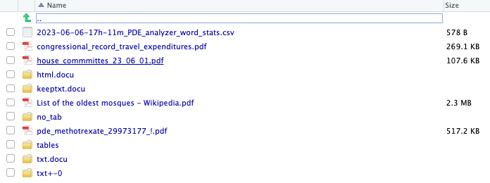
Here you see both the input and the output in the same directory.
- There are different directories for text and tables.
You can manually review the data by navigating through the directories.
7.20.2.3.2 Open the Reader
The Reader GUI allows you to review the output and annotate it by moving through the files.
- It also allows you to open up a PDF folder and TSV file to reanalyze a document.
The vignette has examples of the types of actions you can take.
Both {tabulapdf} and {PDE} are general packages for working with PDFs so there is substantial cleaning to do.
They both appear to work best for small tables that are clearly labeled as “Table”.
They do offer an alternative if copy and paste into a document or spreadsheet is not working well.
If you can access the an original document on the web, it might be easier to scrape it using custom code, than convert to PDF and scrape the PDF with a general use package.
7.21 Scraping Dynamic Web Pages with the {RSelenium} Package
April 2025. The websites in this section have recently been updated so the code will not work as it has to be updated to accomodate the changes in CSS and structure.
It remains as a guide for a strategy to use RSelenium but the code has been turned off until the section can be updated.
7.21.1 Introduction
This is a case study on using using the {RSelenium} package for scraping the Indian E-Courts website, an interactive and dynamic web site.
This case study uses multiple techniques for using Cascading Style Sheet selectors to identify different kinds of elements on a web page and scrape their content or their attributes to get data.
The functions in what follows are not documented nor do they include error checking for general use. They are designed to demonstrate how one can scrape data and tidy/clean it for analysis for this site.
This web site in this case study is constantly evolving to new page designs and uses different approaches and standards for similar designs.
The functions here worked on the test cases as of early June 2023. However, if the test web pages are changed or one is scraping additional district courts for different acts, it could lead to errors if they are using a different design or page structure.
The user should be able to compare the code for these test sites, for old and new designs, and use their browser Developer Tools to Inspect the attributes of the elements on the erroring page, to develop updated solutions.
The E-courts website allows users to search for and gather information on local and district civil court cases for most Indian states.
- There are many thousands of possible cases so the site is interactive as it requires users to progressively identify or select the specific attributes for the cases of interest to limit how much data is provided so users get the information they want.
- The site is dynamic in that as a user makes selections, e.g., the state, the court, the applicable law(s), the web page will update to show the next set of selections and eventually the data based on the selected attributes.
- The website also incorporates a requirement to solve a Captcha puzzle to get to the actual cases.
- Including a Captcha is designed to force human interactivity and keep bots from being able to scrape everything automatically.
The case study focuses on getting data on court cases based on the states, judicial district, court, and legal act (law) for the cases. The E-courts site allows for search by other attributes such as case status.
The site has a separate web page for each district of which there are over 700.
- There are two different designs for district sites.
- The older design redirects to a services site for searching for cases using a dynamic page.
- The newer design embeds the dynamic search capability from the service site into the district page.
- The sites have different structures but similar attributes for the data of interest.
This diverse structure of many pages and dynamic pages means the strategy for scraping data must handle navigating to the various pages and accommodating the different designs.
The strategy uses {RSelenium} to provide interactivity and {rvest} to access and scrape data. The strategy has three major parts:
- Get Static Data: Use {rvest} and custom functions to access and scrape static pages about states and districts which create the URLs for the state-district dynamic pages.
- Get Dynamic Data - Pre-Captcha: Use {RSelenium}, {rvest} and custom functions to interact with the website to access and scrape data up to the requirement to solve the Captcha.
- Get Dynamic Data - Post-Captcha: Use {RSelenium}, {rvest} and custom functions to interact with the website once the Captcha is solved to access and scrape data.
7.21.1.1 The {RSelenium} Package
The {RSelenium} Package Harrison (2023a) helps R users work with the Selenium 2.0 Remote WebDriver.
The Selenium WebDriver is part of the Selenium suite of open-source tools for “automating all major web browsers.”
- These tools are designed to help developers test all of the functionality of their website using code instead of humans.
- The automating part is about using code to mimic the actions a human could take when using a specific web browser to interact with a webpage.
- Actions includes scrolling, hovering, clicking, selecting, filling in forms, etc..
Since developers want to test their sites on all the major browsers, there is a three-layer layered structure to provide flexibility for different browsers but consistency in top-level coding for the developer.
- At the top layer, a developer writes R code to use {RSelenium} functions to represent human interactions with a web page using a browser.
- In the middle layer, the {RSelenium} functions use the Selenium WebDriver standards to interact with “driver” software for the browser.
- At the lower layer, the browser “driver” interacts with the specific brand and version of browser for which it was designed.
- As the webpage (javascript) responds to the requested actions, it communicates updates back up the layers to the R code.
- RSelenium allows the developer to observe the dynamic interactions on the web site through the browser.
Each brand and version of a browser, e.g., Chrome, Firefox, etc., has its own “driver” software, e.g., Chrome Driver for Chrome and Gecko Driver for Firefox.
The Selenium construct is for testing if the website code operates in accordance with its specifications.
It does not test if humans will actually like or be able to use the web site.
Testing the user experience (UX) is a whole other specialty in web site design. Institute (2023)
7.21.1.2 Setup for Using the {RSelenium} Package
- Setting up to use {RSelenium} can be a bit complex as you have to have matching versions of software for each of the three layers (R, Driver, Browser) and the software has to be in the right location, which is different for Windows and Mac.
- Update all the software:
- Update to the latest versions of RStudio and the {Rselenium} package.
- Update your Java SDK to the latest version. See Java.
- Update your browser to the latest version. Recommend Firefox or Chrome.
- Install the correct driver for the browser you want to use.
- If using Firefox, install the gecko web driver for your version. Go to https://github.com/mozilla/geckodriver/releases/.
- For a Mac with homebrew installed, you can use
brew install geckodriver.
- For a Mac with homebrew installed, you can use
- If using Chrome, you need the version number to get the correct web driver.
- Open Chrome and enter the following to see the installed version
chrome://version/version. - Go to https://sites.google.com/chromium.org/driver/ and download the matching version.
- Open Chrome and enter the following to see the installed version
- If using Firefox, install the gecko web driver for your version. Go to https://github.com/mozilla/geckodriver/releases/.
Google is deprecating the old chromedriver. The supported way forward is to use Chrome for Testing (CFT), which ships with a matching chromedriver.
This following steps explain how to set it up on macOS (Apple Silicon) and Windows for use with RSelenium.
7.21.1.3 Installing Chrome or Testing on macOS (Apple Silicon)
Download Chrome for Testing - Get the mac-arm64 build from Google: Chrome for Testing. The homebrew version may be out of date.
Install Chrome for Testing - Move the app into Applications using the terminal
mv ~/Downloads/chrome-mac-arm64/chrome-mac/ "/Applications/Chrome for Testing.app"
- The path to the binary is now
/Applications/Chrome for Testing.app/Contents/MacOS/Chrome for Testing.
Install Chrome Driver sing the terminal .
sudo mv ~/Downloads/chrome-mac-arm64/chromedriver-mac-arm64/chromedriver /usr/local/bin/
sudo chmod +x /usr/local/bin/chromedriver
- You will need to enter your password.
- Test in the terminal with
chromedriver --version. You will probably get a security warning from the Mac.
- Use
sudo xattr -d com.apple.quarantine /usr/local/bin/chromedriverto change the status and retest.
- When ready use the following in your R code.
7.21.1.4 Installing Chrome or Testing on Windows
Download Chrome for Testing. Get the win64 build from: https://googlechromelabs.github.io/chrome-for-testing/
Extract Chrome for Testing. Unzip. You’ll see:
chrome-win/ chrome.exe chromedriver-win64/ chromedriver.exe
Move chromedriver to PATH. Copy chromedriver.exe to a folder in your PATH, e.g.:
C:\Windows\System32\Test with powershell
chromedriver --versionWhen ready, point to it in your R code.
- Test with the Firefox browser using the code below with the {httpuv} package to get a random unused port.
- You will need to install {httpuv} using the console.
- Setting
check= FALSEwill prevent it from checking for the formerly-free netstat port.
library(RSelenium)
# start the Selenium server and open the browser
my_port <- httpuv::randomPort()

rdriver <- rsDriver(
  port    = my_port,
  browser = "firefox",
  check   = FALSE
)

# create a "client-user" object to connect to the browser
obj <- rdriver$client

# navigate to the url in the browser
obj$navigate("https://wikipedia.org/")

# close the browser
obj$close()
# remove the test objects from the environment
rm(obj, rdriver)
7.21.2 Scraping Strategy Overview
Accessing the court cases requires knowing the state, the judicial district, the court, the act(s) (laws), and case status of interest.
The scraping strategy was originally designed to collect all of the courts for each state and judicial district and save them for later collection of the acts for each court.
- This design assumed the data would be stable in terms of the court names and option values. However, experience has shown the assumption is incorrect as they change rather frequently.
- The functions below have not incorporated error checking yet so if a court option value changes it causes an error and the process steps.
- Thus the strategy was revised to identify only the courts for a given state and judicial district and then get the acts for those courts. This reduces the opportunities for errors.
- The process below now saves the data for a state, district, and court along with the acts to a
.rdsfile with the codes for the state and district. There are hundreds of these files. - The process also incorporates a random sleep period between 1-2 seconds between each state/district to minimize the load on the web site.
- Scraping the acts for the almost 10,000 states, districts, and courts can take multiple hours.
Scraping the Data takes place in three steps.
7.21.2.1 Get Static Data
The base e-courts site is interactive but static. Users interact to select states and districts.
The web pages have data needed to create URLs for accessing the state and district and district services pages. Custom functions are used to scrape data and create URLs. The data saved to an .rds file.
7.21.2.2 Get Dynamic Data - Pre-Captcha
Each Judicial District has links to the “Services Website” search capability which is interactive and dynamic.
- This is where the user has to make selections on the specific courts, acts, and status of cases of interest.
- Web scraping gathers all of the options for the various kinds of courts and the many laws.
- Since the website is dynamic, the code uses {RSelenium} to navigate to each state-district URL.
- The two types of court and specific courts of each type are scraped for each state and district combination.
- Each court has its own set of acts that apply to its cases.
- The acts data for each is scraped.
- Each state-district combination has its own data set of court types, specific courts, and acts. This data set is saved as an individual .rds file (several hundred of them).
This step ends with the saving of the data given the need to solve a Captcha puzzle to make progress.
While there are options for using code to attempt to break Captcha puzzles, these notes do not employ those methods.
7.21.2.3 Get Dynamic Data - Post-Captcha
Getting to the cases requires solving a Captcha puzzle for every combination of state-district-specific court, and acts.
That is a lot of puzzles to be done one at a time.
Thus one should develop a strategy for choosing which combinations are of interest.
- That can involve filtering by state-district, court-type, court, and/or acts.
For each combination of interest, the code navigates to the appropriate site and enters the data up to the acts.
The user then has to choose the type of cases: active or pending, and then the “Captcha puzzle has to be solved.
Once the Captcha puzzle is solved, the site opens a new page which provides access to the case data.
- The case data can be scraped and saved or further analysis.
7.21.2.4 Manipulatng the Data
Once the data has been scraped, there is code to help manipulate the data for additional analysis or scraping.
- One can read in all the files into a single list.
- Then one can reshape that list into a data frame with a row for each state, district and court and a list column of the acts.
- Then one can identify a vector of key words for filtering the acts.
- Then one can filter the acts for each court to reduce the number of acts.
- Finally one can unnest the acts.
7.21.3 Step 1. Get Static Data
7.21.3.1 Getting Data for States and Judicial Districts
We start with the top level web site page, https://districts.ecourts.gov.in/ which has an interactive map showing each state.
- Each state name is a hyperlink with a URL to open a page with an interactive map for the state showing the judicial districts in the state.
- Note: The judicial districts do not align exactly to the state administrative districts. In several cases, multiple administrative districts are combined into a single judicial district.
- The URLs for the state web pages use abbreviated state names.
- The district names are also hyperlinks with a URL to open a page with administrative information about the judicial district.
- The old design for a district page has a panel on the right for
Services.- The
Case Status/Actis a hyperlink with a URL to open a new page the “services” website (base URLhttps://servces.ecourts.gov.in) for the selected state and district. - This is the starting web page for interacting with the site to select courts, acts (or laws) and eventually cases.
- The
- The new design for a district page has an icon for Case Status which contains a link for
Actswhich opens up an embedded search capability from the services site.
7.21.3.2 Load Libraries
7.21.3.3 Get States and Judicial Districts
7.21.3.3.1 Build Helper Functions
This step builds and tests several help functions to get the text or the attributes from an element.
- Set the root level url.
- Define a function for scraping text from a URL.
- Define a function for getting the HTML attributes of a selected object from a URL.
7.21.3.3.2 Scrape the official state names and state URL names.
Scrape the official state names.
- Inspect the web page to get the CSS selector for the div with
class="state-district" - That div is a parent of children list items, one for each state with the tag
afor hyperlink. - Scrape the names using the combined selector for parent and child of
".state-district a". - Rename the scraped names and save to a data frame.
Scrape the state URL names.
- The state URL names are abbreviated.
- They appear the values of the
hrefattributes of the children list items for each state.- The
hrefvalues are designed to be the last part of a URL so each comes with a/on the front end.
- The
- Append the
state_url_nameto the end of the site root URL for a complete URL for each state. - Write the code so as to start with binding the
states_dfto the result, by columns, and save.
7.21.3.3.3 Scrape the state pages to get the official district names and URLs.
Scrape the district names and URLs for each state and save as a list-column of data frames.
Append the scraped url to the end of the root URL to get a complete URL for the page.
Note the
map()progress bar in the console pane.
url_ecourts <- "https://districts.ecourts.gov.in"
district_state_css <- ".state-district a"
states_df |>
  mutate(state_district_data = map(state_url, \(url){
    #bind_cols(
      scrape_text(url, district_state_css) |>
        rename(district_name = value)#,
      (scrape_attrs(url, ".state-district a") |>
        unlist() |>
         as.vector()) |>
        tibble(district_url_name = _) |>
        mutate(district_url = str_c(url_ecourts, district_url_name, sep = ""))
   # )
  }, .progress = TRUE)
  ) ->
states_districts_ldf
7.21.3.3.4 Scrape district pages to get the URLs for their Services page.
- Given the two different design for the district web pages, the layout and list structure for each district are **not* the same.
- The newer sites embed the services site into the page and others open a new window with the services site.
- However, both designs use of the attribute
title="Act"for the link to the services page. - The selector for a named attribute uses
'[attribut|="value"]'(see The Ultimate CSS Selectors Cheat Sheet) - Note the use of single and double quotes.
The two designs also differ in the value of the href for the services search capability.
- The old design site provides a complete “absolute URL” since it is opening up a new page in a new window.
- The older design uses numeric codes for state and district in the URL.
- The newer design site is a redirect from the older-style district URL to a new site.
- Instead of an absolute URL, it uses an internal “relative URL” to refresh the page with the embedded search capability now showing.
- This relative URL must be appended to the “canonical URL` defined in the head of the web page to navigate to the page.
- The results are different style URLs for districts and states.
- Most states have an active search capability but not all.
- About 53 districts have an “empty” link to the services site (0s in the code fields) so you cannot search for cases based on the acts for those districts.
7.21.3.3.4.1 Build a helper function to get the canonical URL for a page.
7.21.3.3.4.2 Build a function to get the services URL given a base district URL and the css for the services link.
Since there are still more older design district pages than newer, only get the canonical URL if required for a new design page.
- Use
css = '[title|="Act"]'for both new and older design web pages. - The structures above the list items have different classes but using the title attribute skips ignores them in searching the DOM.
Test the function get_s_d_url() on one or more districts with the css = '[title|="Act"]'.
7.21.3.3.4.3 Scrape the data and unnest to get state and district service URLS and codes where they exist.
Update the list-column of district data with the services URLs
- Unnest to create a wider and longer data frame.
- Extract the state and district codes for the older design URLs.
map(states_districts_ldf$state_district_data, \(df) {
    df$district_url |>
     map_chr( \(url) get_s_d_url(url, '[title|="Act"]')) |>
          tibble(state_district_services_url = _) ->
        temp
   bind_cols(df, temp)
  },
  .progress = TRUE
  ) ->
  states_districts_ldf$state_district_data

states_districts_ldf |>
  unnest(state_district_data) |>
  mutate(
    state_code = str_extract(state_district_services_url, "(?<=state_cd=)\\d+"),
    district_code = str_extract(state_district_services_url, "(?<=dist_cd=)\\d+")
  ) ->
states_districts_df- Write the states district data to
"./data/states_districts_df.rds".
This completes the scraping of static data.
7.21.4 Step 2. Get Dynamic Data - Pre-Captcha
In this step, the goal is to capture all the possible courts within each State and Judicial District and then capture all the possible acts that apply to each court.
That data can be then used to select which states, districts, courts, acts, and status to be scraped after solving the Captcha puzzle.
7.21.4.1 The Services Web Site is Interactive
The services site allows one to search for information by court and act and status on a web page for a given state and district.
There are two types of court structures: Complexes and Establishments in a district. They have different sets of courts.
- The services site web pages are dynamic. As the user selects options, the page updates to reveal more options.
- Note: each option has a
value(hidden) and aname(what one sees on the page). - The
valuesare needed for updating the page and thenamesare useful for identifying thevalues.
- Note: each option has a
- The services site URLs use numeric codes for states (1:36) and districts. However, the pages do not contain data on the state or district only the URL does. The linkages between states and URLs were captured in step 1.
The step begins with loading the data from step one for a given state and judicial district.
The user must select a type of court (via a radio button).
Once the type of court is selected, the user has to select a single court option.
- The data is scraped to collect each possible court of each type for the district.
Once the court option is selected, the user can enter key words to limit the possible options for acts.
- The search option is not used below as the goal was to collect all the acts.
- The data is scraped for all possible act option values and names.
- Some courts have over 2000 possible acts.
- Once an act is selected, the user can also enter key words to limit to certain sections of the act in the
Under Sectionsearch box. That is not used in this effort.
At this point the data with all the acts for all courts in a state and district is saved to a file.
Once an act is selected, the user must chose (using radio buttons) whether to search for
PendingorDisposedcases.Once that choice is made a Captcha puzzle is presented which must be solved.
The presentation of the Captcha ends step 2.
7.21.4.2 Build/Test Custom Functions
Let’s start with reading in the data from step 1.
- Read in states-districts data frame from the RDS file.
Let’s build and test functions to get data for each State and District and type of Courts
- Define smaller functions that are then used in the next function as part of a modular approach and a build-a-little-test-a-little development practice.
Define functions for the following:
- Access the pages for each state, district, and type of court.
- Convert each html page into an {rvest} form.
- Scrape Court Names and Values from each form based on the court type of Court Establishment or Court Complex.
- Scrape the specific courts of both court establishments and court complexes for each state and district.
7.21.4.2.1 Access Court Pages as a Form for each URL
Define a function using rvest::html_form and rvest::session to access the page for a URL as a session form.
- The new design has two elements in the form object and we want the second element.
- Test the function with a URL of each design.
Define a function to get court pages as “forms” for a state and district.
- Use the just-created
get_court_page()function.
get_court_pages <- function(.df = states_districts_df, .s_name = "Andhra Pradesh", .d_name = "Anantpur") {
  stopifnot(is.data.frame(.df), is.character(.s_name), is.character(.d_name))

  dplyr::filter(.df, state_name == .s_name & district_name == .d_name) |>
  mutate(ec_form = map(state_district_services_url, \(url) get_court_page(url))) ->
  .df
  .df
}
Test the function get_court_pages().
- Save to a variable
test_pagesto use later on.
The result for each test should be a list-object of with one element which has class form.
The form elements are the fields o the form to which one can navigate.
7.21.4.2.2 Use the Form to Make Choices and Access the Data
Define a function to extract court names and values from the page’s form based on type of court structure.
- Handle both types of court structures as they have different form object
names. - Use the names from the fields of the correct form and scrape the option names and values for the select box.
- The first entry is the “Select Court …” default so can be removed.
get_court_data <- function(ec_form, court_type) {
  if (ec_form[[1]][1] == "frm") { # old_design

    if (court_type == "establishment") {
      tibble(
        court_names = names(ec_form$fields$court_code$options)[-1],
        court_values = ec_form$fields$court_code$options[-1]
      )
    } else if (court_type == "complex") {
      tibble(
        court_names = names(ec_form$fields$court_complex_code$options)[-1],
        court_values = ec_form$fields$court_complex_code$options[-1]
      )
    }
  } else { # new design
    if (court_type == "establishment") {
      tibble(
        court_names = names(ec_form$fields$est_code$options)[-1],
        court_values = ec_form$fields$est_code$options[-1]
      )
    } else if (court_type == "complex") {
      tibble(
        court_names = names(ec_form$fields$est_code$options)[-1],
        court_values = ec_form$fields$est_code$options[-1]
      )
    }
  }
}
Test the function get_court_data() with test_pages$ec_form.
- The results should be an empty list.
Define a function to extract court establishments and court complexes for a state and district.
- Select the identifying URL and court type and pivot to convert into character vectors of the names and values
- Use a left join to add to the
states_districts_df.
get_courts <- function(.df, .s_name, .d_name) {
  get_court_pages(.df, .s_name, .d_name) |>
  mutate(court_establishments = map(ec_form,
                                    \(form) get_court_data(form, "establishment")),
         court_complexes = map(ec_form,
                               \(form) get_court_data(form, "complex"))) |>
  select(-c(state_district_services_url, ec_form)) |>
  pivot_longer(cols = starts_with("court_"),
               names_to = "court_type",
               names_prefix = "court_",
               values_to = "data") |>
  unnest(data) |>
  ungroup() |>
  unique()  |>  ## get rid of duplicate data in one district court
  left_join(states_districts_df)  |>
  arrange(state_name, district_name, court_type) ->
  tempp
  tempp
}
Test the get_courts() function with examples of old and new designs.
- The result should be data frame with 12 columns and 39 and 42 rows.
Now that the functions are built and tested, they can be used in scraping the dynamic website.
7.21.4.3 Use {RSelenium} Access to Acts for each Court
Load {RSelenium} then start the driver and connect a client-user object to it.
We will use the running server as we build and test functions (that use our previous functions) to access the data in sequence instead of as isolated test cases.
- If you are having to restart due to error or time out of the server you may have to close the server and garbage collect which will close the java server.
- Ref Stop the Selenium server
Use RSelenium::rsDriver() to create a driver object to open the browser to be manipulated.
- Use
netstat::freeport()to identify a free port for the driver to use. - The resulting
rDhas class"rsClientServer" "environment". - Assign a name to the
rDr$clientobject (a remoteDriver) as a convenience for accessing your “user”.
7.21.5 Scope the Scraping for Steps 2 and 3.
Scraping the entire data could take a while since there are 722 districts across the states.
One can filter the data frame to states_districts_df to chose a subset of districts based on state_name and/or `district_name.
- Create a data frame for which states and districts are to be scraped.
- Adjust filters to expand or limit.
# chose states
chosen_states <- unique(states_districts_df$state_name)
set.seed(1234)
chosen_states <- sample(chosen_states, size = 2)

# chose districts
chosen_districts <- unique(states_districts_df$district_name)
set.seed(1234)
chosen_districts <- sample(chosen_districts, size = 5)

states_districts_df |>
  filter(state_name %in% chosen_states) ->
  chosen_states_districts
chosen_states_districts |>
  group_by(state_name) |>
slice_head(n = 3) |>
  ungroup() ->
  chosen_states_districts
Scrape all acts for each court based on the states and districts in chosen_states_districts.
- Open the server if required.
- Scrape all the acts for the states-courts of interest.
Step 2 is now complete.
You can close the driver/browser for now.
All of the acts are saved for all of the courts in the states and districts of interest.
7.21.6 Scope the Scraping for Step 3.
The data from Step 2 is saved in .rds files, each of which is identified by the state and district names.
- Each .rds file contains a data frame with data on all of the courts and their applicable acts for the state and district.
Even without the requirement to solve a Captcha puzzle, one would probably want to filter the data prior to the Step 3 scraping of cases to reduce the volume of data to what is relevant for a given analysis.
Given the Captcha puzzle, one can only scrape for cases for one state, district and court at a time, for a selected set of acts.
However, one can scope the amount of scraping for Step 3 by selecting specific states and districts to be scraped as well as the acts to be scraped. This will greatly reduce the number of cases to just the relevant cases for the analysis.
- The selected states and districts can be a subset for a state-district-focused analysis or a random sample for a broader analysis.
- The selected acts can be based on either specific act names or key words that might appear in an act name.
- Unfortunately, the act names are not consistent across all courts.
- Thus, key words might provide better data (with an initial analysis focused on cleaning the data for consistent names for the analysis).
The following sections demonstrate methods for scoping the data for Step 3 in the following sequence.
Filter by state and District
- Load all the file names saved from Step 2 into a data frame.
- Identify the states and districts of interest.
- Filter by state-district.
- Load in the files for the file names of interest.
Filter the Courts
- Identify the courts of interest for the analysis.
- Filter the data frame based on either
court_typeorcourt_name.
Filter the Acts
- Identify the key words of interest for the acts.
7.21.6.1 Filter by File Name
The data from step two is saved in .rds files each of identified by the state and district codes.
- Load all the file names saved from Step 2 into a data frame and append to the path.
- The
list.files()function retrieves all of the file names in the directory.
- The
- Create a character vector of the states and districts of interest by their names.
- Filter the file names to only those with codes of interest.
- Load in the files for the file names of interest and reshape as a data frame.
# Create list of file names
tibble(file_names = list.files("./data/court_act_rds")) |>
  mutate(file_names = str_c("./data/court_act_rds/", file_names)) ->
 court_act_rds_files

# Create vector of state_district names of interest
my_states_districts <- c("Andhra Pradesh_Anantpur", "Andhra Pradesh_Krishna")

court_act_rds_files |>
  mutate(s_d = str_extract(file_names, "([:alpha:]+\\s?[:alpha:]+_[:alpha:]+\\s?[:alpha:]+)(?=\\.rds)")) |>
  filter(s_d %in% my_states_districts) |>
  select(-s_d) ->
 court_act_rds_files

 ## read in the files of interest
all_acts <- map(court_act_rds_files$file_names, read_rds)- Reshape the list into a data frame with one list-column for act_names.
The court_acts_all data frame now contains all of the acts for the state-district courts of interest.
7.21.6.2 Filter Courts
The court_acts_all data frame has data on all of the courts.
One can filter the data frame based on the variables court_type and/or court_name.
- Let’s assume we only want to filter to “establishment” courts.
- That would leave 46 courts in the data frame.
- We will leave them all in for now.
7.21.6.3 Filter Acts based on Key Words
There are thousands of acts in the data, most of which are probably not of interest for a given analysis.
We can try to scope the data to the acts of interest based on key words.
- Create a vector of key words for the acts of interest.
- As an example, let’s assume the question of interest is about land reform.
- Convert the vector into a regex string.
- Define a function to filter a data frame to the acts of interest based on the key word regex.
- Use
map()to filter each data frame to the acts of interest. - Save the updated data to a file.
- Help from a domain expert will be needed to determine if Land Acquisition Act, Land Acquisition (Amendment) Act , Land Acquisition (Amendment and Validation) Act, and Land Acquisition (Mines) Act are truly different acts or different versions of the same act.
We now have a data frame with the states, districts, courts, and acts of interest for which we want to find cases in Step 3.
7.21.7 Step 3. Get Dynamic Data - Post-Captcha
Given the presence of the Captcha puzzle, Step 3 requires working one state, district, court, and act at a time.
- The cases can have status “Pending” or “Disposed” which must be chosen before the Captcha Puzzle is activated as well.
- There are 722 districts. Each can have between 10 to 30 courts. There are over 2000 acts and an average of 100 plus for each court.
- Thus, there is no practical way to to scrape all of the data for even a single act across all courts and districts. That would require solving thousands of Captcha puzzles.
Many courts do not have any cases for many acts.
- A domain expert might be able to assist in narrowing the parameters for a given question of interest.
The question of interest will shape how to proceed across the various attributes to get to cases of interest
Let’s assume one wants to look for cases under a single Act, “LAND ACQUISITION (A.P. AMENDMENT) ACT, 1953”, that are already Disposed.
Assuming one has identified a small set of states, districts, and courts, the following strategy can help get to and scrape the case data.
7.21.7.1 Strategy
- Create the data frame of attributes of interest (state, district, court type, court, act, case status)
- Start the selenium server web driver.
- Start with the first record of interest.
- Use the client object to navigate to the state-district web page with the services search capability.
- Use functions to make entries for the court type and specific court and the act.
- Use functions to enter the case status.
- Manually enter the Captcha solution.
- In many cases the response is “No records found.” If so, record that result, and move to the next entry.
- If cases are found, a new page will open. Scrape the data and save to a file.
- Move to the next record of interest.
7.21.7.2 Preparing for the Captcha
7.21.7.2.1 Create the Data Set
Let’s create a test case for state “Andhra Pradesh”, district “Anantpur”, all courts, act “LAND ACQUISITION (A.P. AMENDMENT) ACT, 1953” and disposed cases.
- Read in the data for the state and district courts and acts.
- Unnest and ungroup the acts data frame.
- Filter to the “LAND ACQUISITION (A.P. AMENDMENT) ACT, 1953”
- Use an index variable,
indextto select row of interest for each column and create variables for the attributes of interest
Create a variable for the first part of the file name for the cases.
7.21.7.2.2 Create Functions to Enter Act and Case Status
The functions in this section have only been developed and tested on old-design web pages. Updating the functions to the new design is an exercise left to the reader.
Define a function to enter acts after a court is entered.
enter_act <- function(act_value) {
  act_value2 <- str_replace_all(act_value, '\\"', "")
if (court_type == "complexes") {
  act_box <- remDr$findElement(using = 'id', value = "actcode")
  # act_box$clickElement()

} else {
  radio_button <- remDr$findElement(using = 'id', value = "radCourtEst")
  # radio_button$clickElement()
  # option <- remDr$findElement(using = 'id', value = "court_code")
}
#
## Update act item
 option <- remDr$findElement(using = 'xpath',
                             str_c("//*/option[@value = ", act_value2, "]", sep = "")
                             )
option$clickElement() ## fire change for act )
}
Define a function to enter case status.
enter_status <- function(status) {
  if (status == "Pending") {
    ## Get pending Cases
    radio_button <- remDr$findElement(using = "id", value = "radP")
    radio_button$clickElement()
  } else {
    ## Get Disposed Cases
    radio_button <- remDr$findElement(using = "id", value = "radD")
    radio_button$clickElement()
  }
}
Test enter_act()and enter_status().
- Open Selenium for testing
- The individual lines can be run and the user has to choose whether to run the pending cases or disposed cases.
- Then manually enter the captcha solution and go to the next code chunk.
7.21.7.3 Take action on the Browser via the Selenium server.
Open Selenium Server.
Enter the data to be scraped.
7.21.7.4 Scrape Cases
Once the captcha has been solved, the cases can be scraped with the following function
- Requires an active Selenium server where the court and act have already been entered.
Build a function to get a data frame with identification details for each case.
get_cases <- function() {

case_table <- remDr$findElement(using = 'id', value = "showList1")
case_table$getElementText() |>
str_extract_all("(?<=\n).+") |>
  tibble(data = _) ->
  tempp
tempp |>
  unnest_longer(data)  %>% # need to use to support the "." pronoun
  mutate(table_col = rep_len(c("c1", "versus", "c3"), length.out = nrow(x = .))) |>
  mutate(case_no = ((row_number() + 2) %/% 3) ) |>
  pivot_wider(names_from = table_col, values_from = data) |>
  mutate(sr_no = as.integer(str_extract(c1, "^\\d+ ")),
         case_type = str_extract(c1, "(?<=^\\d{1,3}\\s).+ ")) |>
  separate_wider_delim(cols = case_type, delim = " ",
                       names = c("case_type", "temp"),
                       too_many = "drop") |>
  mutate(petitioner = str_extract(c1, "(?<=\\d{4}\\s).+"),
         respondent = str_extract(c3, "^.+(?= Viewdetails)"),
         case_number = str_extract(c3,
                                   "(?<=Viewdetails for case number\\s).+")) |>
  select(sr_no, case_type, petitioner, versus, respondent, case_number) |>
  mutate(state_district_services_url = state_district_services_url,
         court_type = court_type,
         court_value = court_value,
         act_value = act_value,
         case_status = case_status,
         .before = 1) -> tempp
}
Scrape the case data for all the cases that are returned.
- Scrape the data frame of cases.
- Build a function to view the details of each case.
- Test the
view_case()function.
- The result should be the site opens the second page with details for the case that looks like Figure 7.26:
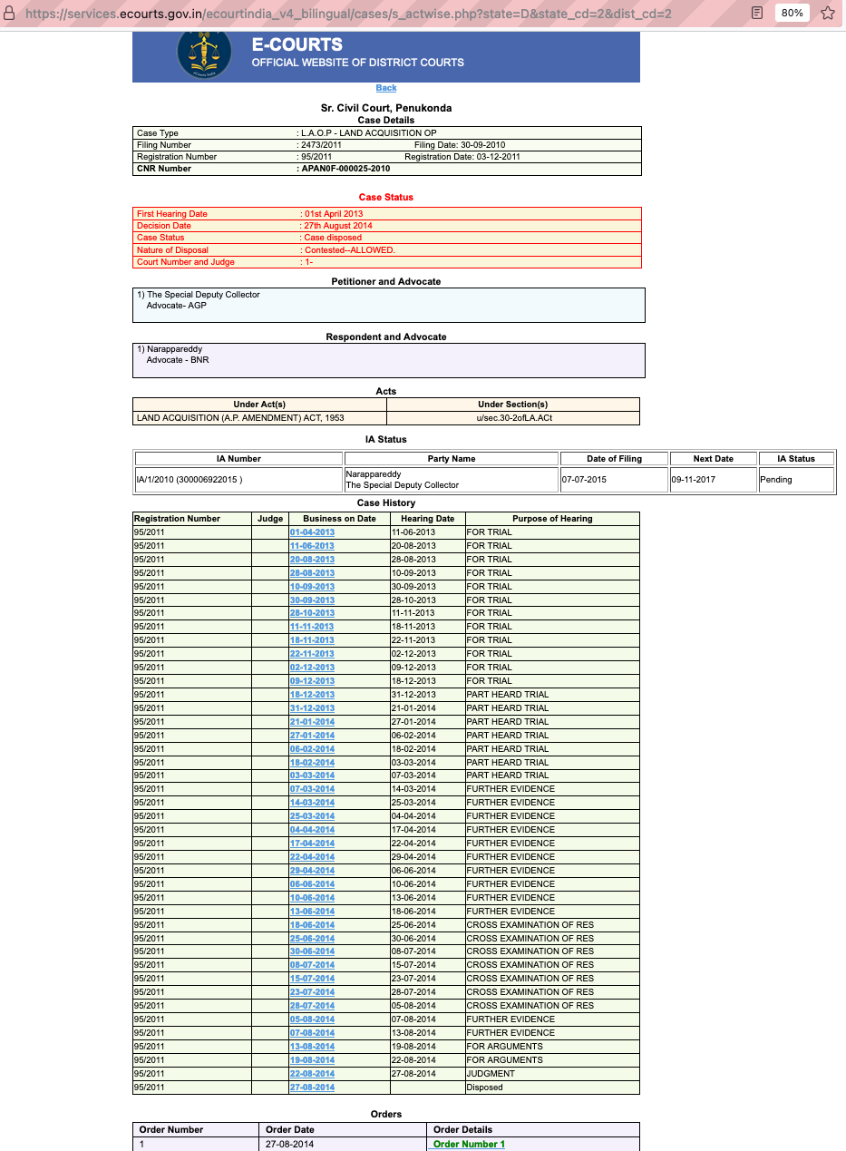
Build a function to get the case details, save, and return (go back) to the first page for the next case.
This function only tidy’s the data into a data frame with a list-column of data frames with the data in each table. It does not clean the data in each table. That can be done later when one is sure of the data to be analyzed.
It was observed that some pages use a table structure instead of the list structure therefore consider extracting the table instead of the text. That would require a different approach to tidying.
get_case_details <- function() {
case_details <- remDr$findElement(using = 'id', value = "secondpage")
case_details$getElementText() -> tempp
write_rds(tempp, "./data/tempp.rds")

table_type = c("Case Details", "Case Status", "Petitioner and Advocate", "Respondent and Advocate", "Acts", "IA Status", "Case History", "Orders")

tempp |> tibble(text = _) |>
  unnest_longer(text) |>
  separate_longer_delim(cols = text, delim = "\n") |>
  mutate(t_type = (text %in% table_type),
         t_type = cumsum(t_type),
         t_type = c("Court Name", table_type[t_type])
         ) |>
  filter(text != "") |>
  nest_by(t_type) ->
  tempp2
cnr <- str_sub(tempp2$data[[2]][[9,1]], start = 3)
write_rds(tempp2, glue::glue("./data/court_act_rds/case_details_", f_name, "_",
                     court_type,"_", court_value, "_", cnr, ".rds"))
go_back <- remDr$findElement(using = "css",
                               value = '[onclick*="funBack"]'
                               )
go_back$clickElement()
}
Scrape all the detailed data and save it.
The result will be a list with null elements with a length of the number of cases.
7.21.7.5 Step 3 Summary of Steps
- Read in the data from step 2 for the state and district courts and acts of interest.
- Unnest and ungroup the acts data frame.
- Filter to the Act of interest, here, “LAND ACQUISITION (A.P. AMENDMENT) ACT, 1953”.
- The result is a data frame of district courts for the chosen act.
- Use an index variable,
indextto select row of interest for each column and create variables for the attributes of interest
- Change the index, increment by 1, to work through each row of the data frame.
- Note when a court has no cases of interest.
- Create a variable for the first part of the file name for the cases.
- Open the Selenium Server and browser.
- Enter the data to be scraped into the browser for the state-district services page.
Solve the Captcha and note if there are no records.
If there are records, scrape the data frame of cases.
- Scrape all the detailed data and save it.
7.21.8 Summary of E-courts Scraping.
This case study shows multiple techniques useful in scraping interactive and dynamic sites using {rvest} and {rSelenium} packages.
It also shows several challenges:
- When a site inserts a Captcha puzzle, that injects a manual step and inhibits automated scraping at scale.
- When a site is evolving, there can be major design differences in the pages that require multiple checks in the functions with different code branches to handle the different designs.
- Even when a site has a similar look and feel, if the pages have been built by different developers, they can use different approaches which again result in additional changes to code.
Recommendations:
- Work with a domain expert who understands how the overall system works to better shape the data to be scraped.
- As an example, if the interest is land reform acts, it may not make sense to search for cases under family courts.
- Work with a system technical expert who understands how the overall systems is evolving to better identify the differences in web page design across the site instead of just finding errors.
7.22 Summary of Web Scraping
When you want to analyze data from a web page and there is no download data or API access, you can try to scrape the data using the {rvest} package tools.
- Use SelectorGadget and/or Developer Tools to find the best CSS selectors.
- Download the page once and save.
- Scrape the elements of interest using the CSS Selectors.
- Create a strategy to convert to a tibble that is useful for analysis.
- Execute the strategy, one step at a time.
- Build-a-little-test-a-little, checking the results at each step.
- Look at the data for cleaning and clean what you need.
Use your new data to answer your question!