Rows: 3
Columns: 15
$ id               <chr> "1401.3269v1", "1502.00318v1", "1712.07349v1"
$ submitted        <chr> "2014-01-14 17:43:11", "2015-02-01 21:43:51", "2017-1…
$ updated          <chr> "2014-01-14 17:43:11", "2015-02-01 21:43:51", "2017-1…
$ title            <chr> "Teaching precursors to data science in introductory …
$ abstract         <chr> "Statistics students need to develop the capacity to …
$ authors          <chr> "Nicholas J Horton|Benjamin S Baumer|Hadley Wickham",…
$ affiliations     <chr> "", "", ""
$ link_abstract    <chr> "https://arxiv.org/abs/1401.3269v1", "https://arxiv.o…
$ link_pdf         <chr> "https://arxiv.org/pdf/1401.3269v1", "https://arxiv.o…
$ link_doi         <chr> "", "https://doi.org/10.1080/09332480.2015.1042739", …
$ comment          <chr> "", "", ""
$ journal_ref      <chr> "", "", ""
$ doi              <chr> "", "10.1080/09332480.2015.1042739", ""
$ primary_category <chr> "stat.CO", "stat.CO", "stat.OT"
$ categories <chr> "stat.CO|cs.CY|stat.OT", "stat.CO|cs.CY|stat.OT", "st…6 Getting Data Using APIs
6.1 Introduction
6.1.1 Learning Outcomes
- Identify potential sources for data from federal, state, local and international governments and agencies.
- Use R tools for interacting with Application Programming Interfaces (APIs) to obtain data from the web and other sources.
- Apply {tidyr} functions to assist in tidying JSON data obtained from a web API output.
6.1.2 References:
- {keyring} R package Csardi (2022)
- {httr2} R Package Wickham (2023)
- {tidycensus} R Package Walker and Herman (2023b)
- {jsonlite} R Package Ooms (2014) Ooms (2023)
- {tidyr} Rectangling Vignette Wickham et al. (2023)
6.1.2.1 Other References
6.2 Governmental Open Data
On Jan 14, 2019, the Foundations for Evidence-Based Policymaking Act of 2018 became law.
Known as the “Open Data Law”, it requires federal agencies to publish their information online as “open data”, using standardized, machine-readable data formats, with their metadata included in the Data.gov catalog.
The Federal Government Data Catalog has metadata on over 250,000 databases available for public use. Most are from state and local governments but there are many from the Federal level or international sources.
The topics cover a wide range of government functions.
The data catalog has links to web sites or repositories from the sponsoring agency.
In many cases, the data is not produced by the source but is curated by an organization as part of an international arrangement, e.g., meteorological or oceanic data.
6.2.1 Federal Government Web Sites
Most Departments, Agencies, and Offices of the federal government have their own websites for providing open data and/or use the central catalog.
- These websites often have tools for visualizing the data as well as downloads.
- Downloads options can include multiple formats: e.g., zip, csv, html, or Excel as well as special formats for mapping data.
- Many sites allow for direct download via your browser while others may require FTP for large data sets.
Some Sites Are Specialized; Others use data.gov
- Census Bureau for data on US people and economy, as well as mapping data.
- Department of Agriculture
- Department of Commerce
- Department of Defense
- Department of Education
- Department of Energy - A spreadsheet
- Department of Health and Human Services
- Department of Justice
- Department of Labor links to the data.gov site with filters set to DOL
- May be faster to go to the Bureau of Labor Statistics
- Department of State
- Department of Transportation takes you to the data.gov catalog
- Other sources of “data”, e.g., Library of Congress can provide cultural context for the nouns and numbers.
6.2.2 Local Government Open Data Initiatives
Many locales have publicly-available data. A few examples:
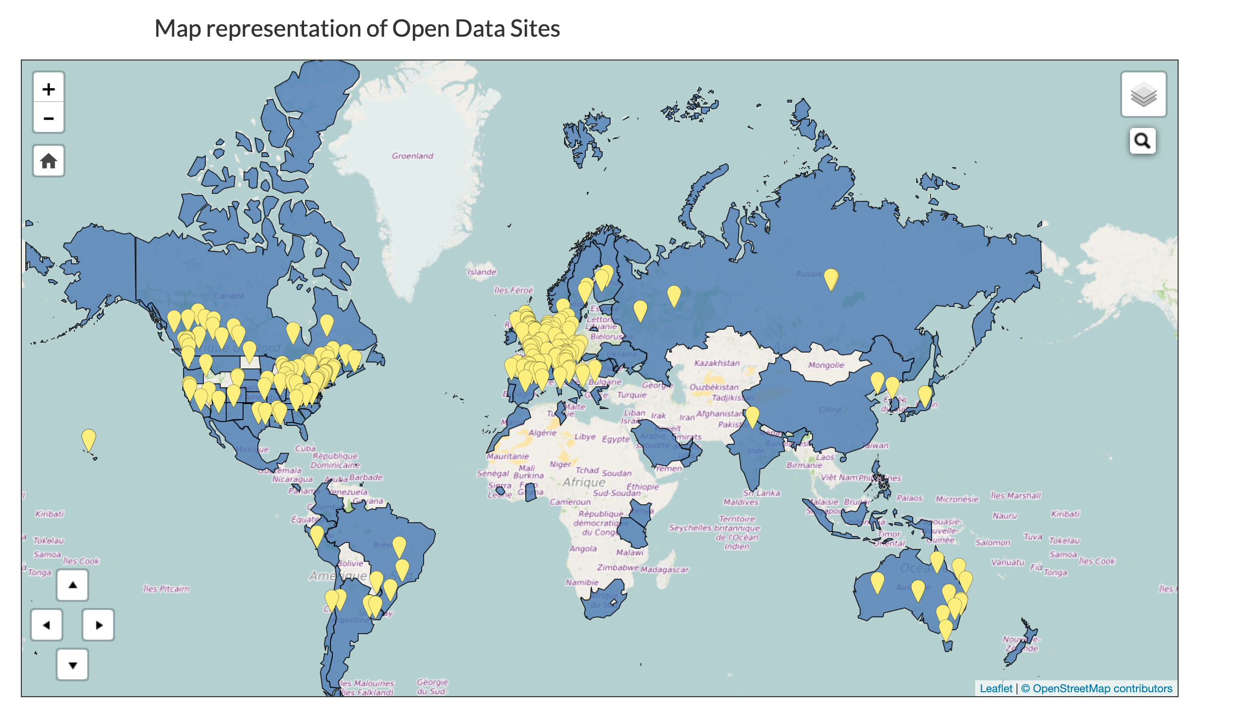
6.2.3 Open Data exists in, or for, Many Countries.
6.2.4 Organizations Sponsor Open Data Sites (some charge a fee)
6.2.5 Bottom Line: Data, Data Everywhere
with Billions and Billions of Bytes to Think
with apologies to Samuel Taylor Coleridge
6.3 APIs and Authentication
6.3.1 Accessing Data on the Web
Nohe (2017)
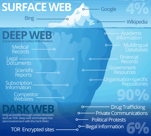
If you think of the web as an iceberg, Open Data is the 4% above the water level.
- This where web-crawlers and search engines roam freely, the surface web . Like an iceberg, there is much more data below the surface - in the deep web.
- This data is protected behind firewalls or application programming interfaces where general search engines (or you) can’t access it without additional steps to establish your identity.
Organizations limit access to their data for many reasons:
- They want want to know who is accessing it (so they can prohibit excess usage).
- They want to protect data integrity (security), intellectual property, or privacy.
Below the Deep web is about 6% of the data in the “Dark Web”, protected by special browsers and routers.
- We will not be working at all with the “Dark Web”.
There are at least four ways to access data via the web:
- Click on a link to download a .csv/.xlsx/.txt/.json/.XML/… file.
- Use a package to interact with an API.
- Write code to interact directly with an API.
- Scrape from directly from the HTML file.
We know how to do 1; this class is about doing 2 and 3 and next class is about 4.
6.3.2 What is an API?
When organizations put their data behind an Application Programming Interface (API) on the Deep Web, they are using software to act as a gateway to control the access to the data.
- A common form of API is known as the Representational state transfer or REST API.
- This architecture is especially useful accessing data as a transaction through public-facing APIs.
APIs can control Who can access, What can be accessed, How can it be accessed, When it can be accessed, and What is returned.
- An API Endpoint is a location of a resource to be accessed by an API (think of an endpoint as aligned with a specific URL).
- APIs may act as gateways to many different endpoints which can be turned open or closed.
Organizations typically publish an API description document to provide users information on how to interact with the API.
- A “how to” guide for requesting data from a particular API (and endpoint), and a description of what type of response you get after the request.
These days, most API will return data in one of two formats:
API’s are an abstraction and can be implemented in many programming languages.
- Think of it like a user interface for a computer program.
- You click a button and expect the user interface to do something.
- An API lets a program click a metaphorical “button” and it expects to get something back.
There are lots of free and public APIs: https://github.com/public-apis/public-apis
- Remember this link for the homework if you can’t think of a site.
Important
Most APIs use common internet communication protocols and data structures.
However, they implement them differently so each API and each API wrapper package will be unique.
You have to read the documentation.
6.3.2.1 Example with Arxiv.
arXive[https://arxiv.org/] is a free distribution service and an open-access archive for nearly 2.4 million scholarly articles in the fields of physics, mathematics, computer science, quantitative biology, quantitative finance, statistics, electrical engineering and systems science, and economics. Materials on this site are not peer-reviewed by arXiv.
The arXiv API is designed to enable efficient searching and retrieval of its huge collection of articles using query keywords.
- One can use it to access metadata about all of the papers on arXiv as well as the papers themselves.
The is an R package called {aRxiv} (Karthik and Broman 2023) which wraps the AIU to provide easier access for R users.
The following example uses {aRxiv} to find all of the arXiv scholarly articles which have Hadley Wickham as an author and are in the “stat”(istics) category.
- Note that the output from the package function is a ready-to-use R data frame.
- The package has other search arguments to customize your search
- The package has additional functions for working with the articles it retrieves.
6.3.3 Authentication
Organizations differ in the level of control they establish for their APIs.
- Some APIs are fully open and do not require any identification or authentication, e.g., the arXiv API in the example above. They may have terms of service to guide your usage but they do not require you to identify yourself.
- Some APIs require you to register your email address so they know who is using their data.
- The next level of greater control is basic authentication where you establish a username and password with the API owner for using the API.
- Many APIs, especially for commercial organizations and US government agencies, now require more advanced authentication such as establishing a Personal Access Token or Access Key.
- Finally, some organizations require you to register as a “developer” and request permission to use their data. They can issue multiple unique authorization tokens/keys for each “app” you are developing to govern your access and the access of any of your “App” users.
Organizations will typically provide documentation on their required level of control and how you gain access to using the API.
6.3.3.1 Basic Authentication
Some API’s use what’s called “Basic” authentication, where you provide a username and password. The basic syntax for this is:
- You can usually apply for a username and password.
- Keep your password secure using the {keyring} package functions and variable names as discussed below.
6.3.3.2 API Keys and Personal Access Tokens
More secure APIs now require you to obtain an API key or personal access token (PAT) credential to establish your identity.
- You may also have to register as a developer.
Important
- Once you get a key, you are responsible for all behavior associated with your key.
- Never save or display your private key in a file you might share such as a R script, .qmd, or .Rmd file.
There are two main ways to store your key so you can access it in R.
- Storing it in your
.Renvironfile. This approach is easy and does not depend on other libraries to access the key but it leaves your key exposed in a plain text file. - Using the {keyring} package. This approach requires installing the package and interacting with your computer credential manager but it keeps your key/password protected at the same level as your computer.
6.3.3.3 Example: Getting an API Key for OMDB
OMDB is the Open Movie Datbase, an open source for information on movies maintained by volunteers. The site is not endorsed by or affiliated with IMDb.com.
OMDB requires you to register your email to obtain a key to use the API.
- Sign up for a free key at: https://www.omdbapi.com/apikey.aspx.
- You should get an email from OMDB with the key.
6.3.3.3.1 Option 1 (Easy but Not Very Secure): Use the .Renviron File to Store and Access Your Key or PAT
This is safer than pasting your key into an .qmd or .R file which you might share.
- Make sure you have the {use_this} package installed on your computer (comes with {devtools}).
- Use the console to open up your .Renviron file using the {usethis} package function
edit_r_environ()e.g.,usethis::edit_r_environ() - Enter the following in your .Renviron:
OMDB_API_KEY = <your-private-key>- “OMDB_API_KEY” is the key name you chose for your key and
- “
” is the key OMDB sent you in the email.
- Restart R.
- You can now always access your private key using the function:
Sys.getenv(key_name), e.g.,Sys.getenv("OMDB_API_KEY").
6.3.3.3.2 Option 2 (More Secure): Use the {keyring} Package to Store and Access Your Key or PAT
Using .Renviron means your key is still in a plain text environment in hidden but unsecure file.
Add a layer of security by using the {keyring} package: https://github.com/r-lib/keyring.
- This puts the key into your computer’s key and credential manager for storage.
- Use the console to install the {keyring} package if you do not have it already:
install.packages("keyring"). - Load the {keyring} package using
library(keyring).
Use the console to save the key into your computer’s login credential manager using key_set(key_name).
- You only do this once!
- This should bring up a pop-up window where you can paste the key you got from OMDB in their email.
- If asked, say
Allow Always. - Using
keyset("key_name")will save the key in the credential manager with the name you choose for the key, e.g.,key_set("API_KEY_OMDB").- On a Mac it will set the name into the “Where” field which is the Mac Keychain Access field for the “service” in the
key_set()andkey_get()functions.
- On a Mac it will set the name into the “Where” field which is the Mac Keychain Access field for the “service” in the
For this example, use the console to enter key_set("API_KEY_OMDB").
- To access the key, a.k.a. credential, in your code, use the
key_get(key_name)function. - You can do this inside your .qmd or .R file as many times as you need.
- Your key is not exposed either in the file or your .Rhistory.
Note
For Mac Users.
🔑 Managing API Keys on macOS
- Starting in 2023, Apple introduced the Passwords & Passkeys app as the primary user-facing tool for managing passwords and passkeys.
- ⚠️ However, this app does not provide programmatic access to API keys.
- The Keychain Access app is still the underlying secure system for storing and accessing secrets like API keys.
- It supports programmatic access via Apple’s Keychain Services API.
- This makes it the recommended option if you want apps or scripts (e.g., R, Python, Swift) to securely access stored API keys.
🗝️ Viewing and Editing API Keys in Keychain Access
- Open Keychain Access: Press CMD ⌘ + Space, type Keychain Access, hit Enter.
- To Keep it handy: Once open, right-click the dock icon and choose Keep in Dock for easier access later.
- Find your API key: Look under login → Passwords. Double-click the item -> check Show password (enter your Mac password).
⚙️ Adjusting Permissions for Apps (e.g., RStudio)
- In the API key’s detail window, go to Access Control.
- Change permissions to:
- “Allow all applications to access this item” (less secure), or
- Add specific apps like RStudio.app (recommended).
- This ensures that RStudio (or another tool) can retrieve the API key automatically when you run a query, without prompting every time.
Warning
A person with password access to your computer can open your credential manager to see your key.
- If they just have access to your computer and know R and the {keyring} package, they could still get to your key.
- However, using the credential manager with {keyring} is more secure than placing your key in a plain text file like .Renviron.
6.3.3.4 Using Your Key in your Code
You could access your key and save it to a variable in your file, e.g, my_key <- keyring::get_key("my_API_key_name").
- However that exposes your key in the global environment and .Rhistory.
A better approach is to just use key_get(key_name) or Sys.getenv(key_name) inside your API functions to access your credential without creating an intermediate variable.
- There are more details about secure ways to access keys in R in this {httr} vignette on secrets.
6.4 Using the {httr2} Package to Access APIs
Most website APIs use HTTP (Hyper-Text Transfer Protocol). It’s a language for querying and obtaining data.
- The six most common http verbs are :
GET(),PATCH(),POST(),HEAD(),PUT(), andDELETE().
We won’t learn HTTP, but we will use the R {httr2} package to interface with APIs through HTTP.
- The goal of this section is not to provide a comprehensive lesson on HTTP and extracting data using API’s. Rather, this just points you to some resources and gives you some examples.
Every API is different, so you always have to figure out how to interact with a new API.
APIs should have documentation you can read to understand important info:
- What parameters you can send?
- How do you need to send them?
- What data you should get back based on the values of those parameters?
6.4.1 The {httr2} Package
The {httr2} package is a complete rewrite of the {httr} package which is now superseded (not updated).
- The package uses several other packages such as {curl} which provides lower level interfaces using HTTP.
- The R {curl} package uses curl capabilities that you may see mentioned in many online posts about accessing data from URLs.
The new {httr2} package transitions from using a single function, GET(), which was executed immediately, to a family of functions around the concept of a “request” object.
- You will still see evidence of underlying usage of
GET()but you do not have to use it as {httr2} allows you to operate at a higher level.
This family of functions allows you to create a request as an R object so you can work with it and refine your request without always executing it.
Use the console and install the {httr2} package.
Use library(httr2) to load and attach the {httr2} package.
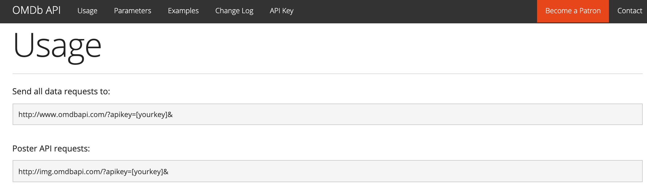
We will use the API for OMDB which is fairly simple and is documented at http://www.omdbapi.com/.
Let’s build a request object and fetch data from OMDB on the movie The Lighthouse.
6.4.2 Building a Request Object
6.4.2.1 Start with the URL
Every request starts with a URL.
- OMDB API documentation says to send all requests to the endpoint “http://www.omdbapi.com/?apikey=[yourkey]&”.
- The terms after
?are the query parameters, so we will just use the base URL to start.
Use request() with the URL and assign a variable name to it.
- To manage the request object we will be using functions that start with
req_....
<httr2_request>
GET http://www.omdbapi.com/
Body: empty- You can see the
GETas the start of the request with the URL but the body of the request is empty.
You can run a “dry-run” to see exactly what will be sent to the URL without sending it.
GET / HTTP/1.1
accept: */*
accept-encoding: deflate, gzip
host: www.omdbapi.com
user-agent: httr2/1.2.3 r-curl/7.1.0 libcurl/8.14.1- The first line is the HTTP method which tells the server what you want to do, along with the protocol version. Here it’s
GETbut it could be other verbs if we were managing a website or posting to a blog. - The host is the URL (stripped of protocol information) and where we will build our query.
- You can modify the additional parameters but we don’t need to do that now.
6.4.2.2 Add Parameters to the Query
We use the req_url_query() function to add name-value pairs to our URL as part of our query, again using the API documentation to define the pair parameter names and possible values.
- The API documentation shows multiple possible parameters:
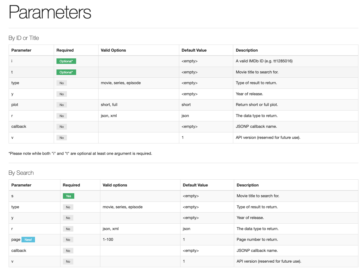
We can build up the query one parameter at a time using the pipe so it is easy to modify.
- Run
req_dry_run()to see what it looks like.
GET / HTTP/1.1
accept: */*
accept-encoding: deflate, gzip
host: www.omdbapi.com
user-agent: httr2/1.2.3 r-curl/7.1.0 libcurl/8.14.1
When you are happy with the request, use req_perform() to actually run the request and then save the response.
6.4.3 Working with the Response
We can see the response object has class httr2_response and displays information we can scan to quickly see what happened.
- First line is the request URL with query.
- Second line is the status code.
- Third line is the Content type. It says
application/json,but it is stored in RAW format. - Fourth line is the size of the body content in RAW form.
[1] "httr2_response"<httr2_response>
GET http://www.omdbapi.com/?t=The%20Lighthouse&plot=short&r=json&apikey=a76d624c
Status: 200 OK
Content-Type: application/json
Body: In memory (990 bytes)The response object is a named list.
- We have seen the
$method,$URL, andstatus_codealready. - We can use the
$headersfor troubleshooting if we absolutely need to withresp_headers(). - The content we want is in the
$body. Note the RAW encoding with 2-character hexadecimal codes.
List of 8
 $ method     : chr "GET"
 $ url        : chr "http://www.omdbapi.com/?t=The%20Lighthouse&plot=short&r=json&apikey=a76d624c"
 $ status_code: int 200
 $ headers    : <httr2_headers>
  ..$ Date                       : chr "Tue, 14 Jul 2026 15:14:28 GMT"
  ..$ Content-Type               : chr "application/json; charset=utf-8"
  ..$ Transfer-Encoding          : chr "chunked"
  ..$ Connection                 : chr "keep-alive"
  ..$ Cache-Control              : chr "public, max-age=3600"
  ..$ Expires                    : chr "Tue, 14 Jul 2026 16:14:28 GMT"
  ..$ Last-Modified              : chr "Tue, 14 Jul 2026 15:14:28 GMT"
  ..$ Vary                       : chr "*"
  ..$ Server                     : chr "cloudflare"
  ..$ X-Aspnet-Version           : chr "4.0.30319"
  ..$ Access-Control-Allow-Origin: chr "*"
  ..$ Cf-Cache-Status            : chr "DYNAMIC"
  ..$ Content-Encoding           : chr "gzip"
  ..$ CF-RAY                     : chr "a1b17a325c017007-IAD"
 $ body       : raw [1:990] 7b 22 54 69 ...
 $ timing     : Named num [1:6] 0 0.0455 0.0714 0.0715 0.1592 ...
  ..- attr(*, "names")= chr [1:6] "redirect" "namelookup" "connect" "pretransfer" ...
 $ request    :List of 8
  ..$ url     : chr "http://www.omdbapi.com/?t=The%20Lighthouse&plot=short&r=json&apikey=a76d624c"
  ..$ method  : NULL
  ..$ headers : list()
  ..$ body    : NULL
  ..$ fields  : list()
  ..$ options : list()
  ..$ policies: list()
  ..$ state   :<environment: 0x848c300b0>
  ..- attr(*, "class")= chr "httr2_request"
 $ cache      :<environment: 0x84e1f7d20>
- attr(*, "class")= chr "httr2_response"- To manage the response we will be using functions that start with
resp_....
6.4.3.1 Check the Status of the Request
The status code describes whether your request was successful.
Use resp_status() to get the code for our request:

Here is a list of some possible status codes.
200 OKmeans our request processed correctly through the API. It does Not mean we got the data we want.204 No Contentmeans our request was accepted but did not return any content.400 Bad Requestmeans the API could not interpret our request.401 Unauthorizedmeans the apikey was not recognized or not validated.408 Time Outmeans it took too long to process due to a slow or broken internet connection.
Codes 204, 400, and 401 mean you should look at the query request and the help documentation for the API to ensure it is correct. Check for typos etc..
Responses with status codes 4xx and 5xx are HTTP errors and {httr2} automatically turns these into R errors.
6.4.3.2 Manipulate the Body Content
There are several resp_body_* functions to convert the content into useful form.
resp_body_raw()shows the raw content in hexidecimal so not so useful for us.
 [1] 7b 22 54 69 74 6c 65 22 3a 22 54 68 65 20 4c 69 67 68 74 68 6f 75 73 65 22
[26] 2c 22 59 65 61 72 22 3a 22 32 30 31 39 22 2c 22 52 61 74 65 64 22 3a 22 52
[51] 22 2c 22 52 65 6c 65 61 73 65 64 22 3a 22 30 31 20 4e 6f 76 20 32 30 31 39
[76] 22 2c 22 52 75 6e 74 69 6d 65 22 3a 22 31 30 39 20 6d 69 6e 22 2c 22 47resp_body_json()converts the RAW content into JSON content with all of the Key:Value pairs.
List of 25
 $ Title     : chr "The Lighthouse"
 $ Year      : chr "2019"
 $ Rated     : chr "R"
 $ Released  : chr "01 Nov 2019"
 $ Runtime   : chr "109 min"
 $ Genre     : chr "Drama, Fantasy, Horror"
 $ Director  : chr "Robert Eggers"
 $ Writer    : chr "Robert Eggers, Max Eggers"
 $ Actors    : chr "Robert Pattinson, Willem Dafoe, Valeriia Karaman"
 $ Plot      : chr "Two lighthouse keepers try to maintain their sanity while living on a remote and mysterious New England island in the 1890s."
 $ Language  : chr "English"
 $ Country   : chr "Canada, United States"
 $ Awards    : chr "Nominated for 1 Oscar. 33 wins & 139 nominations total"
 $ Poster    : chr "https://m.media-amazon.com/images/M/MV5BMTI4MjFhMjAtNmQxYi00N2IxLWJjMGEtYWY1YmU3OTQ0Zjk3XkEyXkFqcGc@._V1_QL75_U"| __truncated__
 $ Ratings   :List of 3
  ..$ :List of 2
  .. ..$ Source: chr "Internet Movie Database"
  .. ..$ Value : chr "7.4/10"
  ..$ :List of 2
  .. ..$ Source: chr "Rotten Tomatoes"
  .. ..$ Value : chr "90%"
  ..$ :List of 2
  .. ..$ Source: chr "Metacritic"
  .. ..$ Value : chr "83/100"
 $ Metascore : chr "83"
 $ imdbRating: chr "7.4"
 $ imdbVotes : chr "301,036"
 $ imdbID    : chr "tt7984734"
 $ Type      : chr "movie"
 $ DVD       : chr "N/A"
 $ BoxOffice : chr "$10,867,104"
 $ Production: chr "N/A"
 $ Website   : chr "N/A"
$ Response : chr "True"resp_body_string()converts the RAW content into a character vector of the JSON Key:Value pairs.
chr "{\"Title\":\"The Lighthouse\",\"Year\":\"2019\",\"Rated\":\"R\",\"Released\":\"01 Nov 2019\",\"Runtime\":\"109 "| __truncated__Here you can see the JSON key:value pairs, e.g.,
"Title\":\"The Lightouse\".If we had used parameter
"r = xml", we could useresp_body_html()to convert the RAW content into an HTML object.You can pipe the response from
resp_body_json(my_resp)toas.data.frame()to convert it to adata.framewhere the$Ratingslist column has been flattened.
Rows: 1
Columns: 30
$ Title            <chr> "The Lighthouse"
$ Year             <chr> "2019"
$ Rated            <chr> "R"
$ Released         <chr> "01 Nov 2019"
$ Runtime          <chr> "109 min"
$ Genre            <chr> "Drama, Fantasy, Horror"
$ Director         <chr> "Robert Eggers"
$ Writer           <chr> "Robert Eggers, Max Eggers"
$ Actors           <chr> "Robert Pattinson, Willem Dafoe, Valeriia Karaman"
$ Plot             <chr> "Two lighthouse keepers try to maintain their sanity …
$ Language         <chr> "English"
$ Country          <chr> "Canada, United States"
$ Awards           <chr> "Nominated for 1 Oscar. 33 wins & 139 nominations tot…
$ Poster           <chr> "https://m.media-amazon.com/images/M/MV5BMTI4MjFhMjAt…
$ Ratings.Source   <chr> "Internet Movie Database"
$ Ratings.Value    <chr> "7.4/10"
$ Ratings.Source.1 <chr> "Rotten Tomatoes"
$ Ratings.Value.1  <chr> "90%"
$ Ratings.Source.2 <chr> "Metacritic"
$ Ratings.Value.2  <chr> "83/100"
$ Metascore        <chr> "83"
$ imdbRating       <chr> "7.4"
$ imdbVotes        <chr> "301,036"
$ imdbID           <chr> "tt7984734"
$ Type             <chr> "movie"
$ DVD              <chr> "N/A"
$ BoxOffice        <chr> "$10,867,104"
$ Production       <chr> "N/A"
$ Website          <chr> "N/A"
$ Response         <chr> "True"
We will see more methods for working with JSON data later.
6.5 R Packages to “Wrap” APIs
Many of the most popular databases/websites already have an R package to “wrap the API”.
The developers have built functions that use familiar R syntax to interact with the API on your behalf and return the data in a form amenable to working in R.
Tip
If an R package exists for an API, you should try it first.
- The developers have tried to make it easier and faster for you to access the data through the API.
- If the R package is missing some functionality you need, you can always use its source code as a guide for developing your own code to interact with the API based on the documentation for the API.
Examples of R packages that wrap APIs:
- Census Bureau APIs: tidycensus
- Ebird API dataset for bird sightings: rebird:
- Geographic location names: geonames
- GitHub REST API: gh
- Spotify API data: spotifyr
- Wikipedia API data: WikipediR
- World Bank Data API: wbstats
- See ROpenSci for many more.
6.6 The {tidycensus} Package
The {tidycensus} package allows users to interact with the US Census Bureau’s decennial Census and every-five-year American Community Survey (ACS) APIs and return tidyverse-ready data frames, optionally with simple feature geometry included. Walker and Herman (2023b)
- We will follow the package tutorial. Walker and Herman (2023a)
There are other Census Bureau API “endpoints” - see Available APIs.
- For our purposes, an endpoint” is essentially a specific URL a system owner has established to enable a user to access a set of data by using an API.
- {tidycensus} has expanded to additional endpoints such as the Migration Flows.
A decennial census may have multiple “Summary files”. See the Census Guidance.
- 2000 Census Summary Files
- 2010 Census Summary Files
- 2020 Decennial Census Redistricting Data
- As of July 2023, only limited data from the 2020 Census, such as the Apportionment and Redistricting data, has been released but more products are on the way. See About 2020 Census Data Products.
There are other R packages for the Census bureau data.
- Hannah Recht’s {censusapi} package enables accessing more Census Bureau APIs or data sets.
- There are other R packages for working with various forms of US Census Data. See A Guide to Working with US Census Data in R section on “How CRAN Can Help”.
6.6.1 Setup
- Install the {tidycensus} package using the console.
- Load {tidyverse} and {tidycensus}.
Important
The tidycensus news for Version 1.8 May 14, 2026 states
Breaking change: the Census Bureau now requires an API key for all requests, including metadata endpoints used by load_variables() and get_pop_groups(). Tidycensus will now error (rather than warn) when no key is available. Pass a key with the key argument or store one for future sessions with census_api_key(“YOUR KEY”, install = TRUE). load_variables() and get_pop_groups() gain a key argument, and table lookups triggered by the table = argument to get_acs() / get_decennial() now forward the resolved key automatically.
Request a key from the US Census Bureau:https://api.census.gov/data/key_signup.html.
- Use your name and email.
- You should get an email in a few seconds.
- Click on the link in the email to activate your key.
- Copy the key from the email - it will be long….
- Set up your key using the console pane:
key_set("API_KEY_CENSUS"). - When queried for a password, use your new key.
- Do not run with INSTALL = TRUE as it will put your key in plain text in your .Renviron file
You could put your key value into a variable but it is better to just use the function key_get() each time e.g., key_get("API_KEY_CENSUS").
6.6.2 Accessing US Census Bureau APIs
The {tidycensus} package has two Main Functions to interact with the Census Bureau’s APIs:
The function get_decennial() grants access to the 1990, 2000, and 2010 decennial US Census APIs as well as the 2020 decennial Census PL-94171 redistricting data.
- Unfortunately, as of 21 Sept, 2020, Error: The 1990 decennial Census endpoint has been removed by the Census Bureau. We will support 1990 data again when the endpoint is updated; in the meantime, we recommend using NHGIS (https://nhgis.org) and the {ipumsr} R package
The function get_acs() grants access to the 5-year American Community Survey (ACS) APIs.
ACS data differ from decennial census data in that ACS data are based on an annual sample of approximately 3 million households, rather than a complete enumeration of the US population.
Thus, ACS data points are estimates with an associated margin of error.
{tidycensus} will always return the estimate and margin of error together for any requested variables when using
get_acs().get_acs()now defaults toyear = 2020to retrieve data from the 2016-2020 five-year ACS. One-year data for 2020 ACS are not yet available in {tdycensus}.Data may be available at multiple levels of resolution or “geographies”, e.g., State, county, tract, etc.. See the full list at Standard Hierarchy of Census Geographies.
6.6.3 First Example - Median Gross Rent
- Let’s look at median gross rent by state in 2000 from the Summary File 3.
- The geography is “state” and the variable is “H063001”.
# A tibble: 6 × 4
  GEOID NAME       variable value
  <chr> <chr>      <chr>    <dbl>
1 01    Alabama    H063001    447
2 02    Alaska     H063001    720
3 04    Arizona    H063001    619
4 05    Arkansas   H063001    453
5 06    California H063001    747
6 08 Colorado H063001 671[1] 52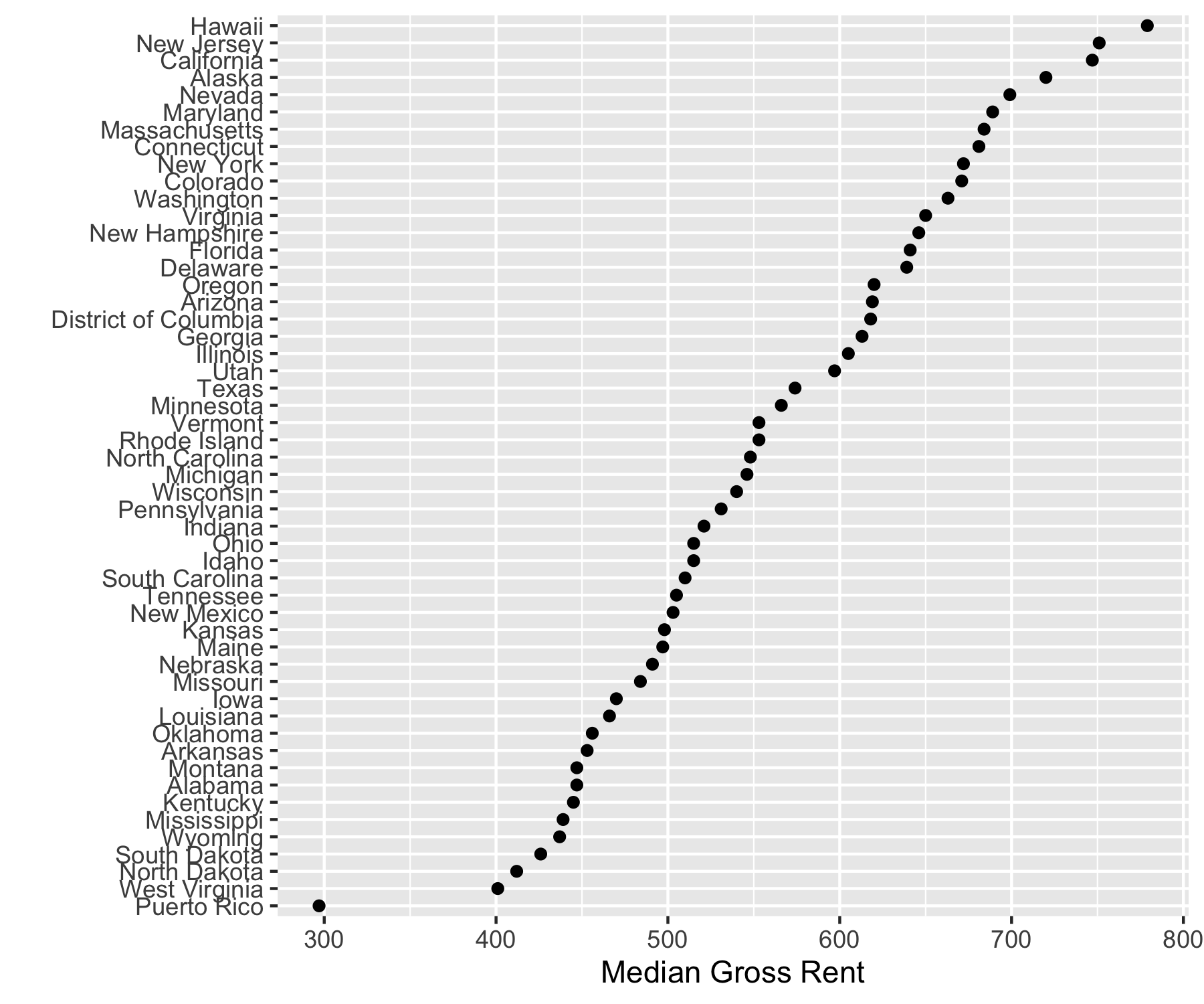
6.6.4 Searching for Census Bureau Variable IDs
There are thousands of variables IDs across the different census bureau files and their IDs are not consistent (but they are configuration managed).
Getting variables from the decennial census or ACS requires knowing the variable ID for the specific product based on the year(s).
To rapidly search for variables, use the load_variables() function.
- Two required arguments:
- the year of the census or the end year of the ACS sample, and
- the dataset: “sf1”, “sf3”, “acs5”, or “acs1”.
- For ideal functionality, assign the output to a variable.
- Then you can use the
Viewfunction in RStudio to interactively browse for variables or usefilter(str_detect())if you know part of the name or concept.
v17a <- load_variables(2017, "acs5", key = keyring::key_get("API_KEY_CENSUS"))
v19a <- load_variables(2019, "acs5",  key = keyring::key_get("API_KEY_CENSUS"))
v00d1 <- load_variables(2000, "sf1",  key = keyring::key_get("API_KEY_CENSUS"))
v00d3 <- load_variables(2000, "sf3",  key = keyring::key_get("API_KEY_CENSUS"))
v10d1 <- load_variables(2010, "sf1",  key = keyring::key_get("API_KEY_CENSUS"))
v20_pl <- load_variables(2020, "pl",  key = keyring::key_get("API_KEY_CENSUS"))
v20a <- load_variables(2020, "acs5",  key = keyring::key_get("API_KEY_CENSUS"))
## v10d3 <- load_variables(2010, "sf3",  key = keyring::key_get("API_KEY_CENSUS"))
6.6.5 Median Gross Rent Continued
Now let’s look at changes over time.
[1] "name" "label" "concept"# A tibble: 0 × 3
# ℹ 3 variables: name <chr>, label <chr>, concept <chr>- Surprise!! There is no median gross rent available for 2010 census.
Let’s jump to the latest data for the ACS 2020 to see if we can find an equivalent variable.
[1] "name" "label" "concept" "geography"# A tibble: 6 × 4
name label concept geography
<chr> <chr> <chr> <chr>
1 B25031_001 Estimate!!Median gross rent --!!Total: MEDIAN… tract
2 B25031_002 Estimate!!Median gross rent --!!Total:!!No bedro… MEDIAN… tract
3 B25031_003 Estimate!!Median gross rent --!!Total:!!1 bedroom MEDIAN… tract
4 B25031_004 Estimate!!Median gross rent --!!Total:!!2 bedroo… MEDIAN… tract
5 B25031_005 Estimate!!Median gross rent --!!Total:!!3 bedroo… MEDIAN… tract
6 B25031_006 Estimate!!Median gross rent --!!Total:!!4 bedroo… MEDIAN… tract # A tibble: 6 × 5
GEOID NAME variable estimate moe
<chr> <chr> <chr> <dbl> <dbl>
1 01 Alabama B25031_001 811 5
2 02 Alaska B25031_001 1240 16
3 04 Arizona B25031_001 1097 5
4 05 Arkansas B25031_001 760 5
5 06 California B25031_001 1586 4
6 08 Colorado B25031_001 1335 6[1] 52Now let’s combine the data frames and plot in sorted order by the 2000 values.
mgr00 |>
  mutate(estimate = value) |>
  bind_rows(mgr20) |>
  group_by(NAME) |>
  mutate(
    delta = 100 * (max(estimate) - min(estimate)) / min(estimate),
    min = min(estimate)
  ) |>
  ungroup() ->
mgr_00_20
mgr_00_20 |>
  ggplot(aes(x = fct_reorder(NAME, min), y = estimate, color = variable)) +
  geom_point() +
  coord_flip() +
  scale_color_discrete(name = "Year", labels = c("2020", "2000")) +
  xlab("") +
  theme(legend.position = "left") +
  ylab("Median Gross Rent") +
  ggtitle("Median Gross Rent") ->
p1
p1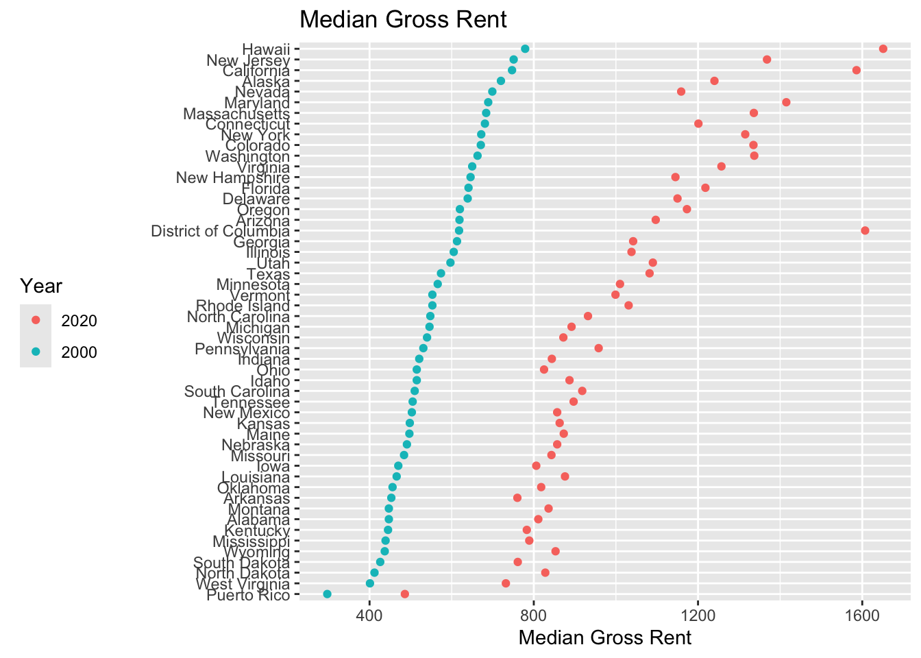
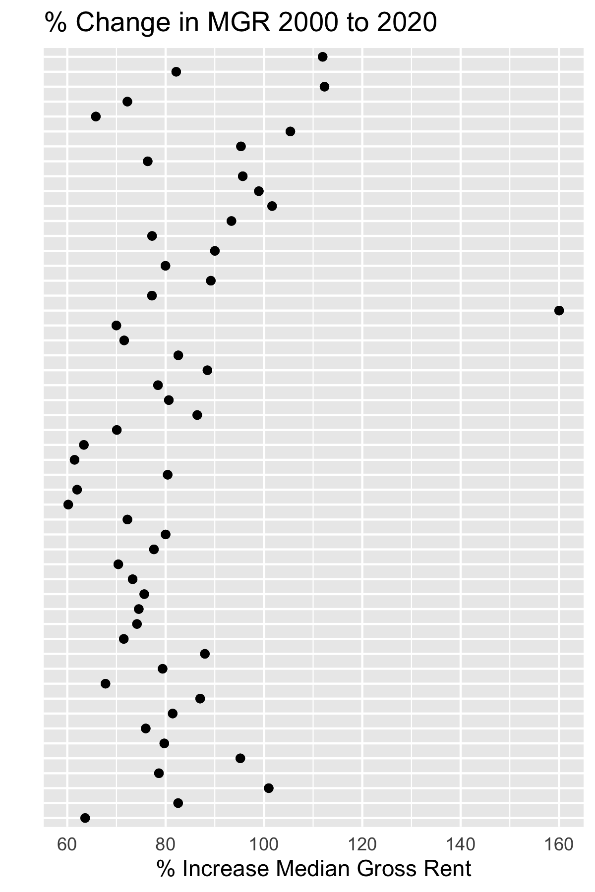
Now let’s combine the data frames and plot the relative percent increase in rent.
mgr_00_20 |>
  ggplot(aes(x = fct_reorder(NAME, min), y = delta)) +
  geom_point() +
  coord_flip() +
  xlab("") +
  theme(
    ## axis.text.x = element_blank(),
    axis.text.y = element_blank(),
    axis.ticks = element_blank()
  ) +
  ylab("% Increase Median Gross Rent") +
  theme(legend.position = "bottom") +
  ggtitle("% Change in MGR 2000 to 2020") ->
p2

p1
p2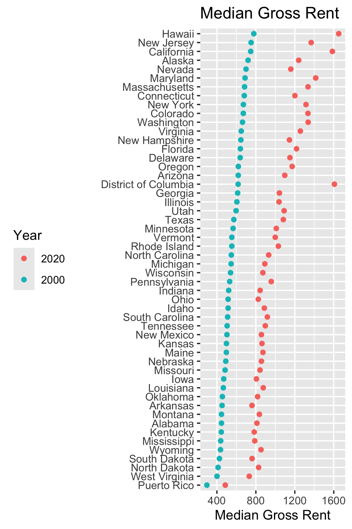
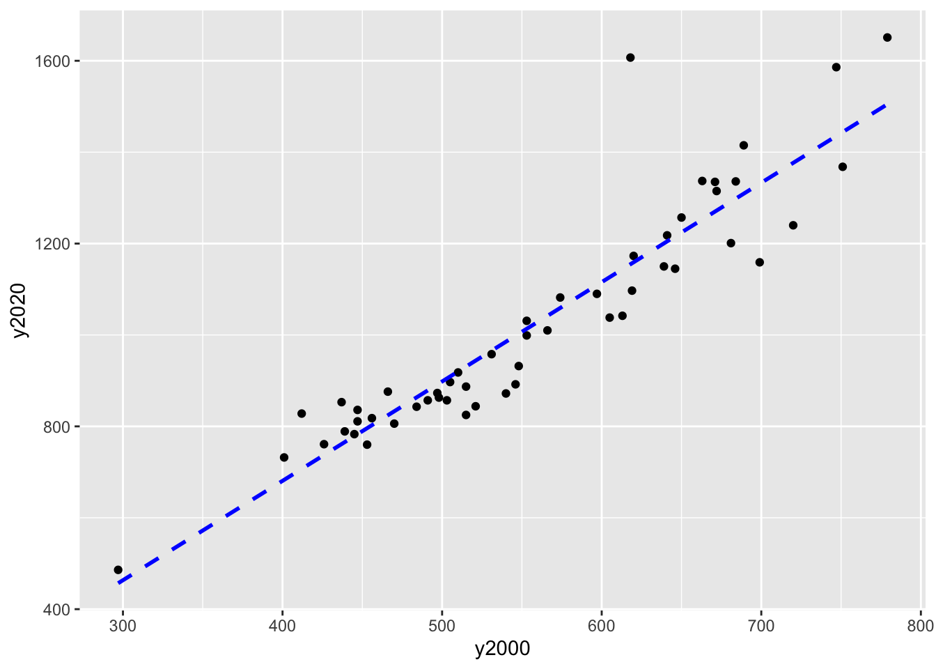
Let’s plot the two years as a scatter plot and add a linear smoother.
mgr_00_20 |>
  mutate(year = ifelse(str_detect(variable, "^H"), 2000, 2020)) |>
  select(-c(variable, value, moe)) |>
  pivot_wider(names_from = year, names_prefix = "y", values_from = estimate) ->
mgr_wide

mgr_wide |>
  ggplot(aes(x = y2000, y = y2020)) +
  geom_point() +
  geom_smooth(se = FALSE, method = lm, color = "blue", lty = 2)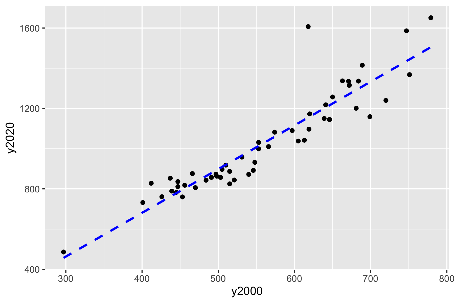
Run a linear model and check the output.
Call:
lm(formula = y2020 ~ y2000, data = mgr_wide)

Residuals:
    Min      1Q  Median      3Q     Max
-171.91  -52.83   -9.86   33.90  452.21

Coefficients:
             Estimate Std. Error t value Pr(>|t|)
(Intercept) -188.9385    72.5423  -2.605   0.0121 *
y2000          2.1743     0.1276  17.035   <2e-16 ***
---
Signif. codes:  0 '***' 0.001 '**' 0.01 '*' 0.05 '.' 0.1 ' ' 1

Residual standard error: 96.19 on 50 degrees of freedom
Multiple R-squared:  0.853, Adjusted R-squared:  0.8501
F-statistic: 290.2 on 1 and 50 DF, p-value: < 2.2e-16# A tibble: 2 × 7
term estimate std.error statistic p.value conf.low conf.high
<chr> <dbl> <dbl> <dbl> <dbl> <dbl> <dbl>
1 (Intercept) -189. 72.5 -2.60 1.21e- 2 -335. -43.2
2 y2000 2.17 0.128 17.0 1.84e-22 1.92 2.43Get the decennial census data for median age by state in 2010, the variable ID is P013001.
Plot the data and reorder the states, on the y axis, by value.
6.6.6 Example: Median Age by Race
Find the variables for median age for both sexes for the 2000 census in the sf1 file from the v00d1 downloaded earlier.
# A tibble: 10 × 2
   name     concept
   <chr>    <chr>
 1 P013001  MEDIAN AGE BY SEX [3]
 2 P013A001 MEDIAN AGE BY SEX (WHITE ALONE) [3]
 3 P013B001 MEDIAN AGE BY SEX (BLACK OR AFRICAN AMERICAN ALONE) [3]
 4 P013C001 MEDIAN AGE BY SEX (AMERICAN INDIAN AND ALASKA NATIVE ALONE) [3]
 5 P013D001 MEDIAN AGE BY SEX (ASIAN ALONE) [3]
 6 P013E001 MEDIAN AGE BY SEX (NATIVE HAWAIIAN AND OTHER PACIFIC ISLANDER ALONE…
 7 P013F001 MEDIAN AGE BY SEX (SOME OTHER RACE ALONE) [3]
 8 P013G001 MEDIAN AGE BY SEX (TWO OR MORE RACES) [3]
 9 P013H001 MEDIAN AGE BY SEX (HISPANIC OR LATINO) [3]
10 P013I001 MEDIAN AGE BY SEX (WHITE ALONE, NOT HISPANIC OR LATINO) [3]
Get the 2000 data for median age for both sexes for White, Black, American Indian/Alaska, and Asian, doing two variables at a time and combining into a single tibble.
Recode variable as a factor with better levels.
Plot median age by Race. How do you interpret the results?
Run an Analysis of Variance to test if all of the Races have the same average median age.
- We have one quantitative response variable (
value) and one categorical (factor) variable (variable). - How do you interpret the results?
             Df Sum Sq Mean Sq F value Pr(>F)
variable      3   2411   803.7   93.64 <2e-16 ***
Residuals   204   1751     8.6
---
Signif. codes: 0 '***' 0.001 '**' 0.01 '*' 0.05 '.' 0.1 ' ' 1# A tibble: 2 × 6
term df sumsq meansq statistic p.value
<chr> <dbl> <dbl> <dbl> <dbl> <dbl>
1 variable 3 2411. 804. 93.6 3.85e-38
2 Residuals 204 1751. 8.58 NA NA Without creating any intermediate variables, let’s find the top 10 entities in terms of the difference between the highest and lowest median ages by Race and plot.
m2000 |>
  group_by(NAME) |>
  summarize(delta = max(value) - min(value)) |>
  slice_max(delta, n = 10) |>
  left_join(m2000) |>
  ggplot(aes(x = fct_reorder(NAME, delta), y = value, )) +
  geom_point(aes(color = variable)) +
  coord_flip() +
  xlab("Entity") +
  ylab("Median Age") +
  scale_color_discrete(name = "Race") +
  theme(legend.position = "top") +
  ggtitle(paste0("Top 10 Entities in terms of the Delta between Max and Min\nacross all Races"))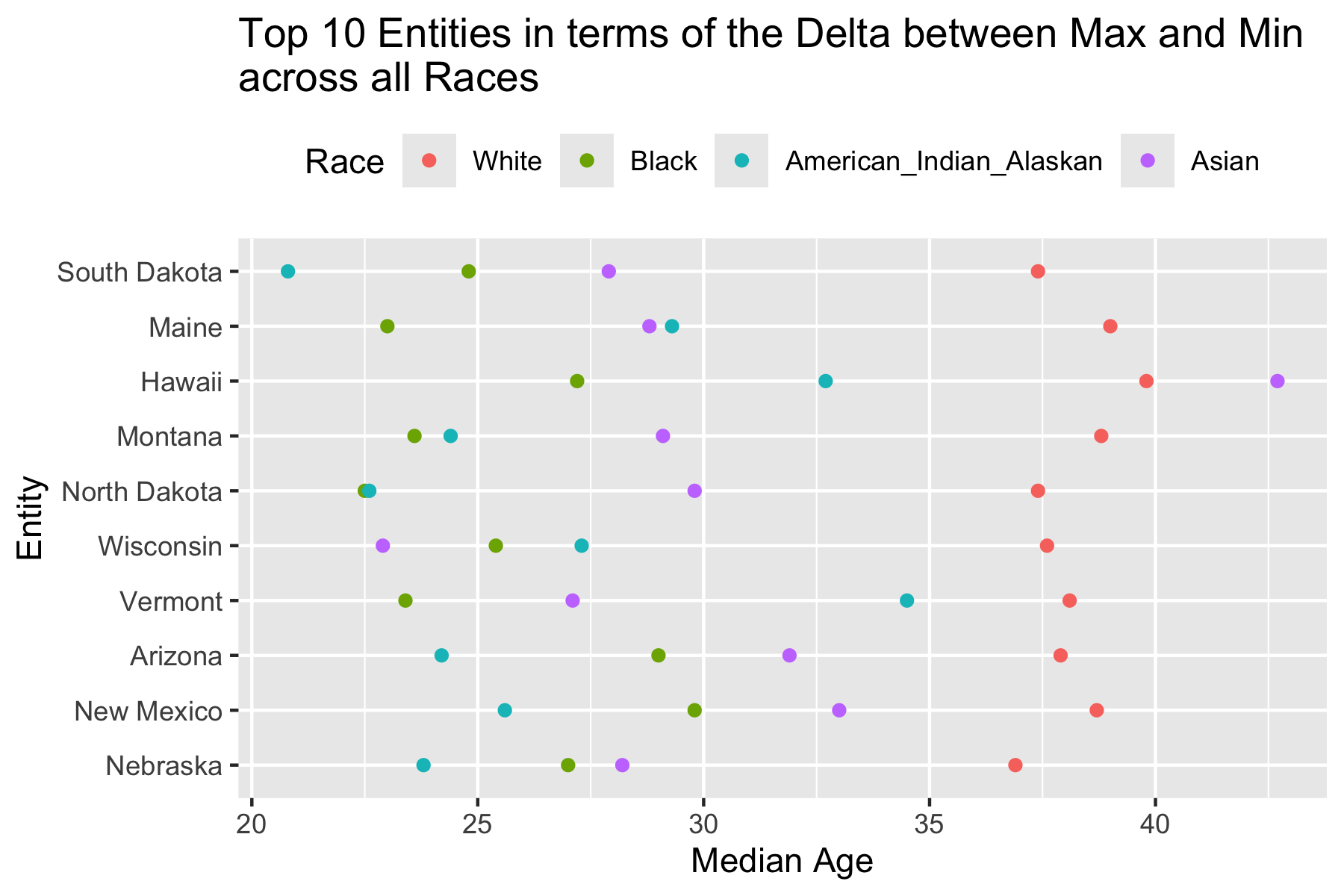
6.6.7 2020 Decennial Redistricting Data
A limited set of variables as required by the Public Law.
# A tibble: 6 × 2
  concept                                                                      n
  <chr>                                                                    <int>
1 GROUP QUARTERS POPULATION BY MAJOR GROUP QUARTERS TYPE                      10
2 HISPANIC OR LATINO, AND NOT HISPANIC OR LATINO BY RACE                      73
3 HISPANIC OR LATINO, AND NOT HISPANIC OR LATINO BY RACE FOR THE POPULATI…    73
4 OCCUPANCY STATUS                                                             3
5 RACE                                                                        71
6 RACE FOR THE POPULATION 18 YEARS AND OVER                                   71
There are only a limited number of concepts.
Let’s look at the concept HISPANIC OR LATINO, AND NOT HISPANIC OR LATINO BY RACE.
- We are not interested in the breakout by Race so we will work with the top level variables.
# A tibble: 3 × 2
  name    label
  <chr>   <chr>
1 P2_001N " !!Total:"
2 P2_002N " !!Total:!!Hispanic or Latino"
3 P2_003N " !!Total:!!Not Hispanic or Latino:"- Note that
P2_001Nis the total ofP2_002NandP2_003N.
Let’s look at the distribution of the percentage of Hispanic or Latino in each county in each state, ordered by total state populations.
- How do you interpret the results?
m2020 <- get_decennial(
  geography = "county",
  variables = c("P2_002N", "P2_003N"),
  year = 2020,
  summary_var = "P2_001N",
  key = key_get("API_KEY_CENSUS")
)
m2020 |>
  separate_wider_delim(NAME, names = c("County", "State"), delim = ", ") |>
  mutate(pct = value / summary_value) ->
m2020
m2020 |>
  group_by(State, variable) |>
  mutate(state_pop = sum(summary_value, na.rm = TRUE)) |>
  ungroup() |>
  filter(variable == "P2_002N") |>
  ggplot(aes(x = fct_reorder(State, state_pop), y = pct)) +
  geom_boxplot() +
  coord_flip()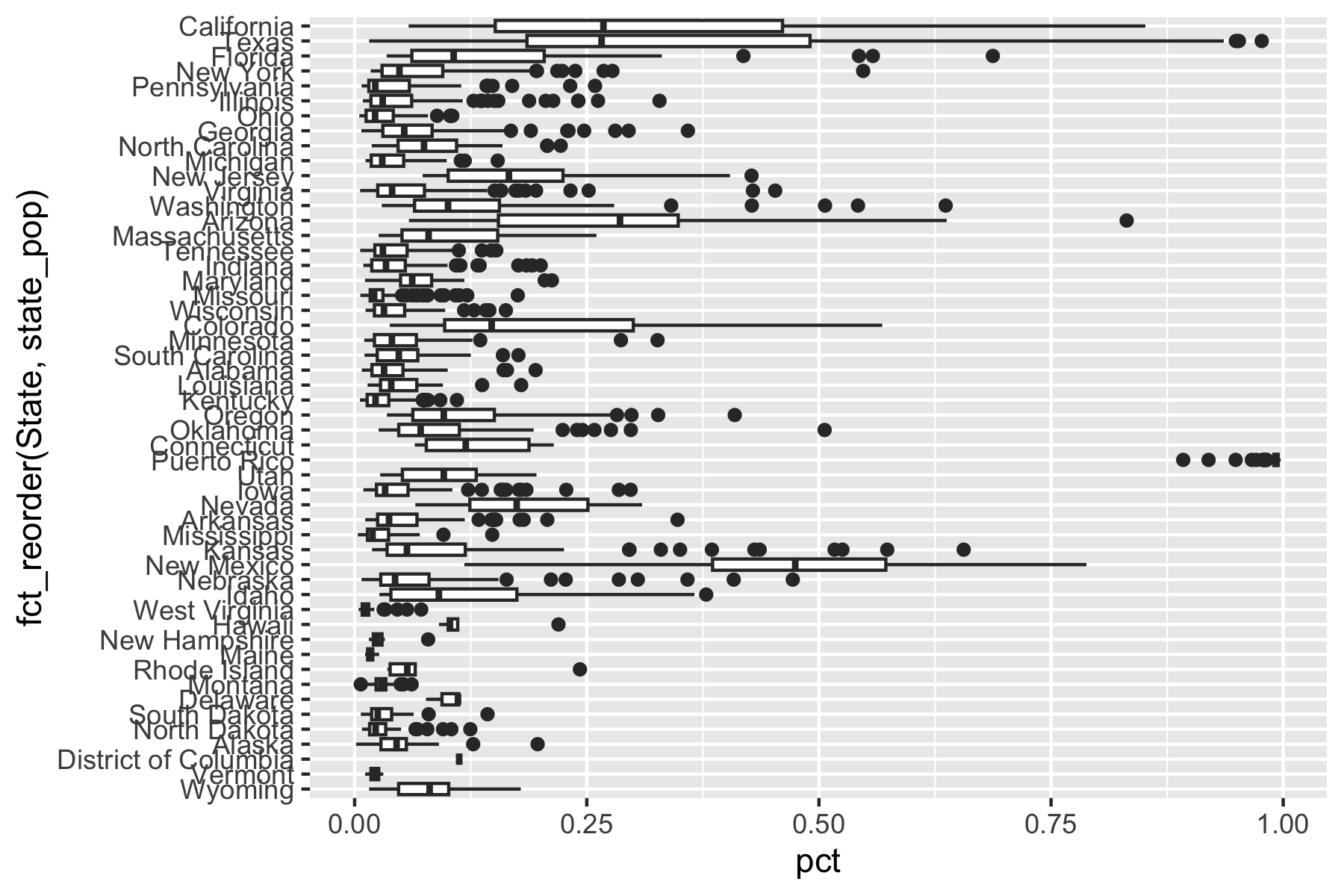
Let’s look at the percentage of Hispanic or Latino in each county by census region.
- Load the census_region_states.csv file from GitHub using https://raw.githubusercontent.com/AU-datascience/data/main/413-613/census_region_states.csv.
- Join with the original data frame and plot by region.
- How do you interpret the results?
census_regions <- read_csv("https://raw.githubusercontent.com/AU-datascience/data/main/413-613/census_region_states.csv")

m2020 |>
  inner_join(census_regions) |>
  group_by(Division, variable) |>
  mutate(div_pop = sum(summary_value, na.rm = TRUE)) |>
  ungroup() |>
  filter(variable == "P2_002N") |>
  ggplot(aes(x = Division, y = pct)) +
  geom_boxplot() +
  coord_flip()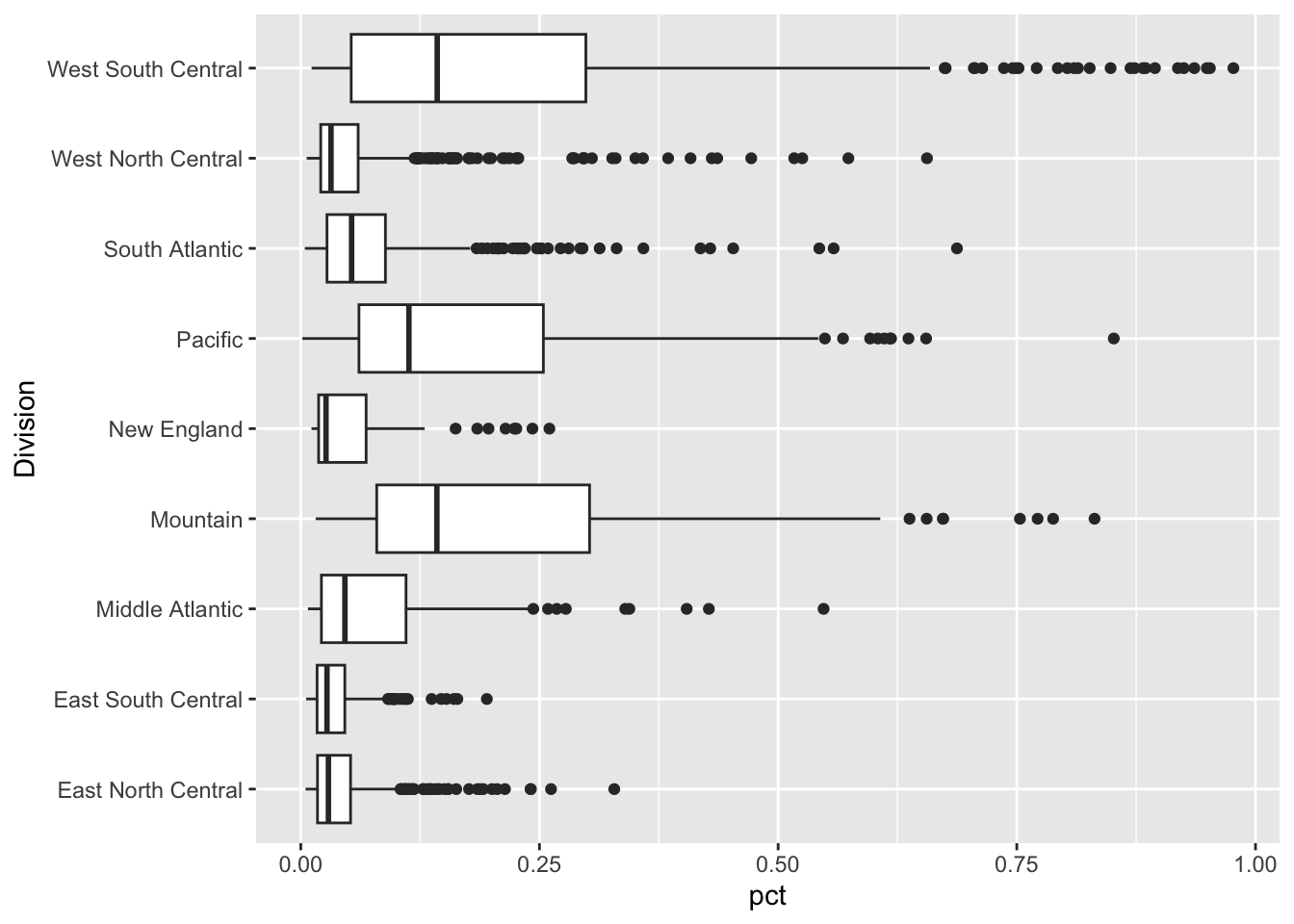
6.6.8 Using get_acs()
Let’s fetch median household income data from the 2016-2020 ACS for counties in Virginia.
# A tibble: 6 × 5
  GEOID NAME                        variable  estimate   moe
  <chr> <chr>                       <chr>        <dbl> <dbl>
1 51001 Accomack County, Virginia   medincome    46178  2575
2 51003 Albemarle County, Virginia  medincome    84643  3217
3 51005 Alleghany County, Virginia  medincome    48513  4275
4 51007 Amelia County, Virginia     medincome    63918  6276
5 51009 Amherst County, Virginia    medincome    57368  4546
6 51011 Appomattox County, Virginia medincome 55457 5246# A tibble: 6 × 5
GEOID NAME variable estimate moe
<chr> <chr> <chr> <dbl> <dbl>
1 51790 Staunton city, Virginia medincome 52292 3116
2 51800 Suffolk city, Virginia medincome 79899 3566
3 51810 Virginia Beach city, Virginia medincome 78136 1419
4 51820 Waynesboro city, Virginia medincome 43480 3487
5 51830 Williamsburg city, Virginia medincome 59288 5801
6 51840 Winchester city, Virginia medincome 61102 4170The output is similar to a call to get_decennial(), but instead of a value column, get_acs() returns estimate and moe (margin of error) columns.
- The
moerepresents (as the default) a 90 percent confidence level around the estimate; this can be changed to 95 or 99 percent with themoe_levelparameter inget_acs()if desired.
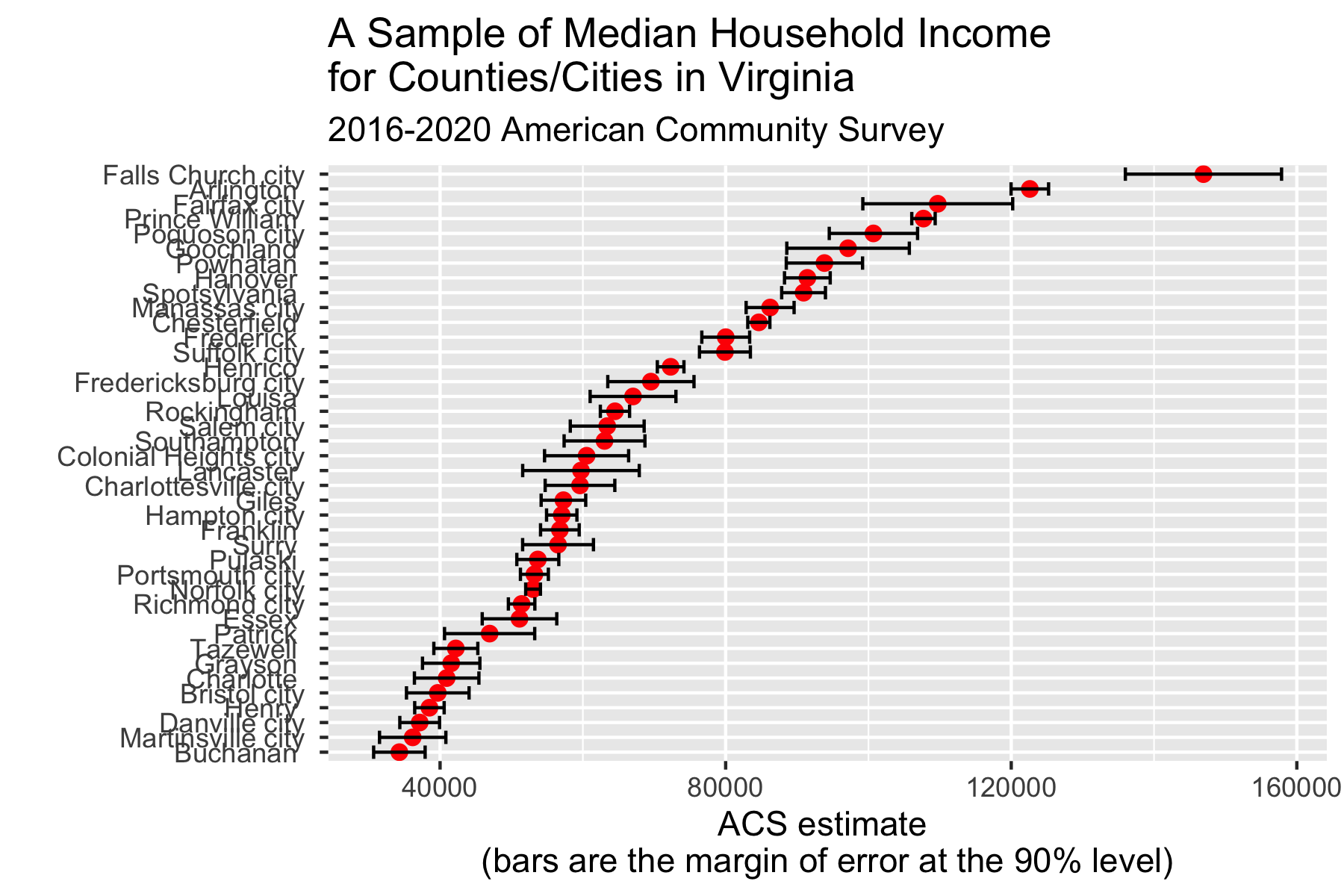
As we have the margin of error, we can visualize the uncertainty around the estimate.
Given the large number of counties and independent cities in VA, let’s randomly sample 40 counties/cities and plot the moe for their median house income.
- How would you interpret the graph?
set.seed(1)
va |>
  mutate(NAME = str_remove_all(NAME, "(County)|(Virginia)|(,)")) |>
  slice_sample(n = 40) |>
  ggplot(aes(x = estimate, y = fct_reorder(NAME, estimate))) +
  geom_point(color = "red", size = 2) +
  geom_errorbarh(aes(xmin = estimate - moe, xmax = estimate + moe)) +
  labs(
    title = "A Sample of Median Household Income\nfor Counties/Cities in Virginia",
    subtitle = "2016-2020 American Community Survey",
    y = "",
    x = "ACS estimate \n(bars are the margin of error at the 90% level)"
  )
6.7 Working with JSON Structured Data
JSON (Javascript Object Notation) is an open-standard text format that is largely replacing XML.
- JSON is completely language independent but uses conventions familiar to programmers for many languages so it’s an ideal data-interchange language.
JSON uses data arrays of attribute-value pairs with multiple data types:
- numbers (double)
- strings (double-quotes)
- boolean (T or F)
- arrays (ordered list, square bracket notation with elements comma-separated)
- null
6.7.1 JSON R packages
There are multiple packages for working with JSON when a download or API returns a JSON file (or you have a URL direct to a JSON file).
- They typically can convert between JSON and a nested R list or data frame.
The rjson package was an early package that has been updated to be faster working with large R objects. It outputs unnamed lists so can be unwieldy.
The jsonlite package is a JSON parser/generator optimized for the web.
- It has bidirectional mappings between JSON data and the most important R data types.
- One can convert between R objects and JSON without loss of type or information, and without the need for any manual data manipulation.
- It also includes functions to stream, validate, and prettify JSON data.
- It’s ideal for interacting with web APIs, or to build pipelines where data structures seamlessly flow in and out of R using JSON.
The {tidyjson} package takes an alternate approach to structuring JSON data into tidy data.frames. Similar to {tidyr}, {tidyjson} builds a grammar for manipulating JSON into a tidy table structure.
We’ll work with {jsonlite} package.
- Use the console to install and then load/attach {jsonlite} using
library().
6.7.2 Simplification in the {jsonlite} Package
Simplification is the process by which JSON arrays are automatically converted from a list into a more specific R class.
- The
fromJSON()function has 3 arguments which control the simplification process:simplifyVector,simplifyDataFrameandsimplifyMatrix.
| Type | Example Jason | Simplifies to | Argument in fromJSON() |
|---|---|---|---|
| Array of primitives, | [“Amsterdam”, “Rotterdam”, “Utrecht”, “Den Haag”] | Atomic Vector | simplyVector |
| Array of objects, | [{“name”:“Erik”, “age”:43}, {“name”:“Anna”, “age”:32}] | Data Frame | simplifyDataFrame |
| Array of arrays, | [ [1, 2, 3], [4, 5, 6] ] | Matrix | simplifyMatrix |
6.7.2.1 Examples for fromJSON() and toJSON()
Simplify is TRUE by default and {jsonlite} works with the structure of the input array to determine what kind of output.
- For an array of like primitives, you get an atomic vector.
[1] "Mario" "Peach" NA "Bowser" chr [1:4] "Mario" "Peach" NA "Bowser"- Turn off simplify and you get a list from any JSON array.
[[1]]
[1] "Mario"

[[2]]
[1] "Peach"

[[3]]
NULL

[[4]]
[1] "Bowser"
When you have a JSON array with key-value pair objects, you can simplify it into a data frame by default.
    Name Age Occupation
1  Mario  32    Plumber
2  Peach  21   Princess
3   <NA>  NA       <NA>
4 Bowser  NA      Koopa
You can convert back with toJSON().
6.7.3 Exercise with the US Congress JSON data
Question: Which gender in congress do you think has the higher average age? Just take a guess. Let’s get some data to see what the data shows.
Get data on the current members of Congress from the @unitedstates project.
- Create a variable
url_congress <- "https://unitedstates.github.io/congress-legislators/legislators-current.json" - Use this as an argument of
fromJSON(). - What is the structure of the output?
A nested data frame with 3 columns of packed data frames and four columns of lists.
Using view() will automatically flatten the structure for viewing in RStudio.
- Notice the variable names for the packed columns are in the form
data-frame-name$column-name, e.g.,id$bioguide.
Rerun with the flatten = TRUE argument. How did the structure change?
An unpacked data frame with 23 columns of data and the same four columns of lists.
Notice the variable names for the packed columns are in the form data-frame-name.column-name, e.g., id.bioguide, where the $ operator has been replaced by a period.
Use {lubridate} functions to convert birthday to a date class and add a column for age in years, convert gender to a factor, add a column for their current term party, and save back to the same data frame.
- Hint: look at help for
time_length(). - Hint: Note that the
$termscolumn is an unnamed list of data frames where each row represents a term in Congress so each party member has different numbers of rows. However, each data frame has$partyas a column of type character. Consider usingmap_chr()withdplyr::last()to extract the last value of$partyfor each member. - Hint: do not try to solve all of these at once. Code one and test it. Then code the next one and test it. and so on.
Who are the three oldest and the three youngest members? Show just the official full name, birthday, gender, and current party.
What is the count by gender? Create a table of counts by gender and current party.
Convert data.
Three oldest and youngest.
Count by gender and table of counts by gender and current party.
Plot the distribution of ages by gender. What do you notice?
Multiple Options
Show code
Each plot shows similarities between the distribution of ages for Females and Males. Both distributions appear symmetric. The violin and box plots have similar medians and the density plots have similar shape and mode. The jitter plot shows similar distribution of points on the Y (age) axis.
Use a t-test to determine if there is a difference between the mean ages of the genders.
6.8 Advanced {httr2} Capabilities for working with APIs
The {httr2} package has multiple functions to help with common situations you might face when getting data using APIs.
- See the package Reference page for details on these functions.
A few common situations include:
- Iterating across multiple queries to get more data than is provided in a single query.
- Iterating across multiple endpoints (URLs) to get more data than is provided with a single query.
- Controlling the rate of multiple queries to avoid exceeding the API’s limits.
- Caching the responses to avoid having to use the API to run the same query.
Important
Many APIs sit behind gateways and rely on supporting search infrastructure (such as Elasticsearch, Amazon OpenSearch Service, or Azure AI Search) so API designers can focus on exposing domain data rather than implementing search systems from scratch. In this architecture:
- A gateway enforces external, policy-driven limits on how clients may call an API.
- The search infrastructure enforces internal, system-configuration limits on how queries can be executed safely and efficiently.
When APIs feel “mysteriously slow or capped,” it is often the interaction of both layers, gateway throttling combined with search-engine query limits, that explains the behavior.
- Gateways protect the overall infrastructure from “abuse” by throttling requests, limiting payload size, or short-circuiting expensive queries.
- See What is Azure API Management? as one example.
- Search Services, e.g., Elasticsearch may restrict deep pagination, aggregation depth, or query execution time to prevent performance degradation affecting multiple users.
Because these controls are policy-driven rather than schema-driven, they are often absent from API reference documentation even though they materially affect performance and behavior.
This is why designing a reliable solution often requires more than reading endpoint specifications.
Empirical testing with edge cases and reviewing platform architecture documentation are essential to understanding real-world API constraint and understanding how to design a reliable, effective solution.
6.8.1 Iterating with APIs
6.8.1.1 Overcoming Response Limits
APIs often place limits on how many records can be returned in a single response, e.g., 100 rows of data.
- To get more data, you will need to submit more than one request in a way to ensure you get the next chunk of data instead of the same chunk you got in the first request.
- Typical API patterns:
?page=2(page-based)?offset=100or?start=101(index-based)?nextPageToken=XYZ(token-based, e.g., Google APIs)
- For many APIs, you can use {purrr} and custom functions to generate multiple queries in sequence.
The {httr2} package has functions to help you Perform Multiple Requests.
- Use
req_perform_iterative()and its helpers to automatically iterate through pages if the API provides standard pagination patterns.
6.8.1.1.1 New York Times Example of Multiple Requests
The New York Times news organization offers an API with multiple endpoints so you as a developer can “programmatically access New York Times data for use in your own applications” (for non-commercial use only).
- There are two rate limits per API: 500 requests per day and 5 requests per minute.
- Sleep 12 seconds between calls to avoid hitting the per minute rate limit.
- To Get Started one creates an account, registers the name of their app, and gets a developer API key and Secret and enables access to specific end points.
The Article Search endpoint allows users to look up articles by keyword and refine your search using filters.
- The API returns metadata for the articles, not the articles themselves.
- It returns a maximum of 10 articles per page.
- You can paginate up to 100 pages (1,000) articles at a time (filter with the date fields to manage getting beyond that using different base queries).
The Article Search uses ElasticSearch Simple Query String Syntax for unfiltered queries, q, and the underlying more complete Apache Lucene Query Parser Syntax for more complex filtered queries, fq.
Note
- Apache Lucene Query Parser Syntax is a compact query language used by many search APIs to express structured search logic for finding relevant records. It includes:
- Boolean operators: AND, OR, NOT combine terms and must be capitalized. Example: whale AND climate
- Fielded searches: restrict terms to specific fields using field:term, e.g.,
news_desk: Science - Grouping with parentheses: control operator precedence, e.g.,
(whale OR dolphin) AND climate
- Fielded searches: restrict terms to specific fields using field:term, e.g.,
- Phrase searches: wrap multi-word phrases in double quotes, e.g.,
"climate change"- Lists of values: fields can match multiple values inside parentheses, e.g.,
Section_name:("Science" "Environment") - Negation: exclude terms or fields with NOT, e.g.,
NOT type_of_material:"Letter"
- Lists of values: fields can match multiple values inside parentheses, e.g.,
- Boolean operators: AND, OR, NOT combine terms and must be capitalized. Example: whale AND climate
- Lucene syntax allows precise, readable queries that combine keywords, field filters, and logical structure—making it well suited for API searches over large text collections.
- The query syntax identifies which records are relevant, while Elasticsearch handles scoring and ranking of the matched results.
ImportantQuoting in R (httr2):
- When passing Lucene queries as strings in R, it is often necessary to mix single (’) and double (“) quotes so that quoted phrases required by Lucene (e.g.,”climate change”) are preserved inside R character strings without excessive escaping.
fq <- 'section_name:("Science" "Environment") AND NOT type_of_material:"Letter"'Once you have stored your API key and loaded the {tidyverse} and {httr2} packages, the following steps will be common to many APIs.
- Use the documentation to define the NYT Article Search endpoint - add the endpoint to the base search URL.
- Define queries of interest, e.g., a compound keyword query (
q) and filter query (fq).
# - Use quotes for phrases, OR to combine phrases
q <- '"climate change" OR "global warming"'

# a Lucene filter query (fq)
# - Restrict to NYT as the source and Focus on specific desks/sections
fq <- 'source.vernacular:"The New York Times" AND (desk:("Science" "Climate") OR section_name:("Science"))'- Build the base request (for the first call) with query parameters Listing 6.1.
- Commonly assigned the name
req. - Use the name by which you stored the API developer key with
keyring::key_set(). - Add the desired query parameters such as
qandfq, dates, sort and starting page. - Use the
req_retry()andreq_throttle()functions to stay within the limits set by the API (and its architecture).- When the API accepts them, they can be more efficient.
- Do not include a
req_perform()step
- Commonly assigned the name
req <- request(base_url) |>
  req_url_query(
    `api-key`  = keyring::key_get("API_KEY_NYT_DEV"),
    q          = q,
    fq         = fq,
    begin_date = "20180101",
    end_date   = "20251231",
    sort       = "newest",
    page       = 0
  ) |>
  req_retry(max_tries = 3) |>  # to automatically retry failing requests
req_throttle(capacity = 5, fill_time_s = 60) # ~5 req/60 sec; - Define a stopping rule. Listing 6.2
- This function is called by
iterate_with_offset()after each request to determine if the$bodyof last response was empty (length == 0).- If so, there are no more pages to be returned, and it stops the iteration.
- Different APIs may need different stopping rules based on how they return the response.
- This function is called by
- Iterate over pages (offset pagination) Listing 6.3
- Start with the base
reqcreated in Listing 6.1. - Use
next-req = iterate_with_offset()for APIs that use indexing such as pages.- Set the
param_name = pagesince that is how the NYT API operates. - Set
resp_complete = is_completeto use the stopping function from Listing 6.2. - The API indexes from
0so setstart = 0. - Advance (offset) by one page at a time.
- Set the
- Set the
max_reqs =to an integer (orInf) for the maximum number of query requests to perform.- This uses 6 to see if the
req_throttle()will be accepted by the API.
- This uses 6 to see if the
- Start with the base
- Using
req_perform_iterative()returns a list of response objects, one for each request or iteration.- They may have class “httr2_response” if successful, or, class “httr2_http_429” if an error.
- Check the list of response objects for their success/status.
- Since the response list may have objects with different classes, it is good to check the class and status for each object before working on the list.
- A successful response object has class ““httr2_response” with status code 200.
- An error response object has multiple classes, including “httr2_error”, and often status code 429 for “too many requests”.
- The
base::inherits()function allows us to check if an element in our list of responses inherits the successful class or the error class. - Saving the output allows us to use it later to subset only the successful responses for additional processing or examine the error responses for what happened.
[1] TRUE TRUE TRUE TRUE TRUE FALSE[1] FALSE FALSE FALSE FALSE FALSE TRUE[1] 200 200 200 200 200 429
NoteUsing
Sys.sleep() if req_throttle() results in errors
In this case,
req_throttle()implements a delay for the limit of five requests in 60 seconds.However, the API returned an object with class “httr2_error” and status 429 (too many tries) on request number 6.
- It also returned the error with the setting of
capacity = 4
- It also returned the error with the setting of
You can try other settings but some APIs can be tricky.
A less efficient perhaps but effective approach is to use
Sys.sleep()to insert a manual delay between each request.A good place to do that is to add it to the stopping rule function from Listing 6.2 since that is run after every request.
Listing 6.4 and Listing 6.5 contain the adjusted code for working with the NYT API limits for the article search end point.
Now we can repeat steps 5 and 6 to run the iteration again and check if we get errors.
Instead of doing so right away, let’s implement a good practice for efficiency when running queries in an interactive setting and debugging later code.
- Note: If you want to run 100 queries, at 5 per minute, it will take at least 20 minutes.
- Start with a small number as you debug your code and save the long query till after you have running code.
TipSave the Results for Subsequent Processing Listing 6.6
- A more efficient approach, especially when working interactively, is to save the output and only run the query if you need new data.
- Save the response list as a compressed Rds file using a relative path to a data folder.
- Use
file.exists()with the same relative path to the data folder - Wrap inside an
if-then-elsestatement to check if the file exists.- If not, run the query to create the response and write it to the .rds file.
- If so, (else), read in the .rds file as name it
response_list.
if (!file.exists("./data/response_list_nyt_api_100_pages.rds")) {
  req_perform_iterative(
  req,
  next_req = iterate_with_offset(
    param_name   = "page",
    start         = 0,
    offset        = 1,
    resp_complete = is_complete
  ),
  max_reqs  = 100,
  on_error  = "return",
  progress  = "NYT pages"
) ->
response_list
  write_rds(response_list, "./data/response_list_nyt_api_100_pages.rds",
            compress = "gz")
} else {
  response_list <- read_rds("./data/response_list_nyt_api_100_pages.rds")
}- Repeat step 6 to check the list of response objects for their success/status.
  [1] TRUE TRUE TRUE TRUE TRUE TRUE TRUE TRUE TRUE TRUE TRUE TRUE TRUE TRUE TRUE
 [16] TRUE TRUE TRUE TRUE TRUE TRUE TRUE TRUE TRUE TRUE TRUE TRUE TRUE TRUE TRUE
 [31] TRUE TRUE TRUE TRUE TRUE TRUE TRUE TRUE TRUE TRUE TRUE TRUE TRUE TRUE TRUE
 [46] TRUE TRUE TRUE TRUE TRUE TRUE TRUE TRUE TRUE TRUE TRUE TRUE TRUE TRUE TRUE
 [61] TRUE TRUE TRUE TRUE TRUE TRUE TRUE TRUE TRUE TRUE TRUE TRUE TRUE TRUE TRUE
 [76] TRUE TRUE TRUE TRUE TRUE TRUE TRUE TRUE TRUE TRUE TRUE TRUE TRUE TRUE TRUE
[91] TRUE TRUE TRUE TRUE TRUE TRUE TRUE TRUE TRUE TRUE [1] FALSE FALSE FALSE FALSE FALSE FALSE FALSE FALSE FALSE FALSE FALSE FALSE
[13] FALSE FALSE FALSE FALSE FALSE FALSE FALSE FALSE FALSE FALSE FALSE FALSE
[25] FALSE FALSE FALSE FALSE FALSE FALSE FALSE FALSE FALSE FALSE FALSE FALSE
[37] FALSE FALSE FALSE FALSE FALSE FALSE FALSE FALSE FALSE FALSE FALSE FALSE
[49] FALSE FALSE FALSE FALSE FALSE FALSE FALSE FALSE FALSE FALSE FALSE FALSE
[61] FALSE FALSE FALSE FALSE FALSE FALSE FALSE FALSE FALSE FALSE FALSE FALSE
[73] FALSE FALSE FALSE FALSE FALSE FALSE FALSE FALSE FALSE FALSE FALSE FALSE
[85] FALSE FALSE FALSE FALSE FALSE FALSE FALSE FALSE FALSE FALSE FALSE FALSE
[97] FALSE FALSE FALSE FALSE [1] 200 200 200 200 200 200 200 200 200 200 200 200 200 200 200 200 200 200
[19] 200 200 200 200 200 200 200 200 200 200 200 200 200 200 200 200 200 200
[37] 200 200 200 200 200 200 200 200 200 200 200 200 200 200 200 200 200 200
[55] 200 200 200 200 200 200 200 200 200 200 200 200 200 200 200 200 200 200
[73] 200 200 200 200 200 200 200 200 200 200 200 200 200 200 200 200 200 200
[91] 200 200 200 200 200 200 200 200 200 200- Convert the list of responses to a tibble
- Identify the successful responses.
- Use
map()to convert each response object’s$bodyto JSON. - Use
map()to extract the element of interest (here$response$docs) from each element and convert to a one-column tibble. - Use
list_rbind()to collapse the list of tibbles into a single tibble.
Rows: 1,000
Columns: 1
$ docs <list> ["The Trump administration has aggressively pulled America away …- Extract the variables of interest from the list column.
- Examine the structure of the list column (here
docs), typically usingview()to identify the name and location for each variable of interest. - Use
hoist()to extract the nested variables into the tibble. - You can chose to remove the original list column or leave it in place.
- Examine the structure of the list column (here
nyt_docs_df |>
  hoist(docs,
    id           = "_id",
    web_url      = "web_url",
    pub_date     = "pub_date",
    section_name = "section_name",
    news_desk    = "news_desk",
    byline = c("byline", "original"),
    headline     = c("headline", "main"),
    abstract     = "abstract",
 snippet = "snippet",
 keywords = "keywords"
  ) |>
  mutate(pub_date = ymd_hms(pub_date)) ->
nyt_docs_df2- Review the data.
Rows: 1,000
Columns: 11
$ id           <chr> "nyt://article/8453e3ec-988c-589e-a244-112a8b814739", "ny…
$ web_url      <chr> "https://www.nytimes.com/2025/12/23/climate/climate-forwa…
$ pub_date     <dttm> 2025-12-23 21:22:21, 2025-12-22 15:08:57, 2025-12-19 17:…
$ section_name <chr> "Climate", "Climate", "Climate", "Climate", "Climate", "C…
$ news_desk    <chr> "Climate", "Climate", "Climate", "Climate", "Climate", "C…
$ byline       <chr> "By David Gelles", "By Brad Plumer, Lisa Friedman, Maxine…
$ headline     <chr> "Looking Back at a Historic Year of Dismantling Climate P…
$ abstract     <chr> "The Trump administration has aggressively pulled America…
$ snippet      <chr> "The Trump administration has aggressively pulled America…
$ keywords     <list> [["Subject", "United States Politics and Government", 1]…
$ docs <list> [[], "article", ["", "An Extraordinary Year of Dismantle…- Explore the Data
nyt_docs_df2 |>
mutate(year = as.factor(year(pub_date)),
month = month(pub_date, label = TRUE)) |>
filter(year != 2020) |>
count(year, month) |>
ggplot(aes(x = year, y = n, fill = fct_rev(month)) ) +
geom_col() +
labs(title = "New York Times Articles on Climate Change or Global Warming",
y = NULL,
x = NULL,
fill = NULL,
caption = "NYT Article API")
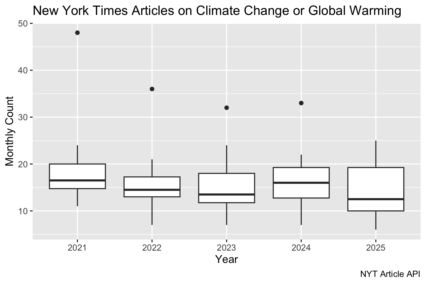
nyt_docs_df2 |>
mutate(year = as.factor(year(pub_date)),
month = month(pub_date, label = TRUE)) |>
filter(year != 2020) |>
count(year, month) |>
ggplot(aes(x = year, y = n)) +
geom_boxplot() +
labs(title = "New York Times Articles on Climate Change or Global Warming",
y = "Monthly Count",
x = "Year",
caption = "NYT Article API")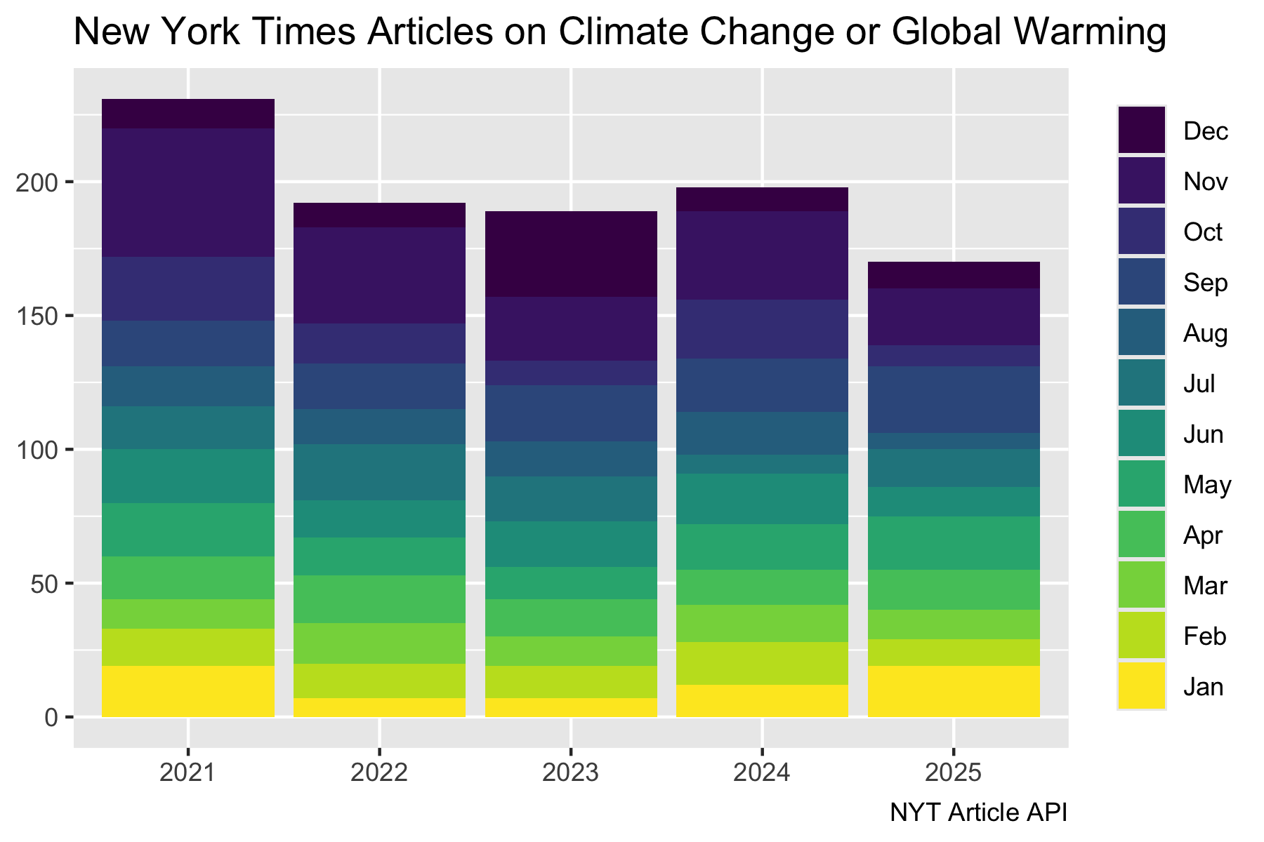
6.8.1.2 Adjusting Endpoint URLs
Some APIs are structured so parameters such as date or location are part of the endpoint URL and not query parameters (after the URL).
- That could mean you have to use different endpoints to get data for different dates or locations.
The {httr2} package has functions to help you Modify Request URL.
- These allow you to adjust a request object and adjust the endpoint URL in the object.
- There are other functions for manipulating URLS outside a request object.
You can use request URL functions to adjust the URL without extra string manipulation.
req_url(): replace the full URLreq_url_relative(): navigate relative to current URLreq_url_path(): set the path directlyreq_url_path_append(): append to the existing pathreq_url_query(): update query parameters
6.8.2 Managing the Request Process
The {httr2} package has functions to help manage the process of submitting queries and working with the responses.
Most APIs set rate limits (e.g., 100 requests/minute).
req_throttle()will automatically add a small delay before each request so you can avoid hitting a server with many requests.- This is a more effective method then just inserting
Sys.sleep()in your functions. - Often the documentation will give it in requests per minute or seconds and if minutes, convert to seconds.
- If you are running multiple large queries in sequence that renders or a script, you may need to put a
Sys,sleep()in between them to avoid error 429: too many requests, as many APIs have undocumented limits to reduce the overall demand on the server in some period of time.
- This is a more effective method then just inserting
It can be time and resource-consuming to repeatedly access the API while debugging code to manipulate the response or rendering your document.
req_cache()creates a cache so if repeated requests return the same results, you can avoid a trip to the server.- It also allows you to adjust parameters to automatically invalidate the cache, e.g., after 7 days.
- When you attach
req_cache("my_cache_dir")to a request, {httr2} computes a cache key based on the full request and then turns that into a hash (like an MD5 digest and stores the response in the designated cache directory under that hash.
Important
The {httr2} req_cache() function only saves responses when they include a complete body that can be written to disk.
- However, many APIs, e.g., the NOAA NCDC API, return responses with
Transfer-Encoding: chunked,which means the server sends the data in pieces instead of a single, fully specified content length. - Because of this, {httr2} cannot determine a stable, cacheable object and nothing is written to the cache directory.
You can confirm this by inspecting the response headers of your initial request:
If you see a value of “chunked”, it means the server is streaming the response in chunks. That prevents {httr2}’s caching from working as intended.
In these cases, the recommended alternatives are to:
- Use Quarto chunk caching (so responses are reused between renders), or
- Implement manual caching (e.g., save JSON or RDS files after each download).
6.9 Additional Examples of Iterating with APIs
This section uses different APIs as examples of getting multiple responses and adjusting endpoints for a given API.
Important
Always review the documentation for an API to determine how best to get your data of interest.
6.9.1 Example of The National Centers for Environmental Information API
The following example shows how to use {httr2} to get data from the National Oceanographic and Atmospheric Administration’s National Centers for Environmental Information using their API.
One of the endpoints has data describing every land-based weather station in the country. However, the API has a limit of 1,000 entities per query and there are over 154,000 records for stations as many stations have multiple entries based on their dates for specific kinds of data availability.
Since the API works on indexes and offsets, let’s get more than 1,000 stations using the req_perform_iterative() and iterate_with_offset() functions.
The API also has other limits for queries per second and total per day.
- Each token (key) is limited to five requests per second and 10,000 requests per day.
httr2:req_throttle()can handle the limit per second but not the limit per day which must be done in other ways.
- Get your National Centers for Environmental Information API key (token) from https://www.ncdc.noaa.gov/cdo-web/token.
- Use {keyring} to store, say as “API_KEY_NCDC”.
- Load the packages and set the base URL and create a variable for the API_limit.
- You have your choice of endpoints for different types of data.
- Let’s get data on the weather stations so we will use the
v2/stationsendpoint.
- Create an initial request.
- The
iterate_with_offset()functions works best with a helper function to determine when all data has been downloaded.
- Let’s create a helper to check how many total records there are and if we have reached it yet.
- The
Sys.sleep()is a hack to slow down the requests so we do not hit the limit of 5 requests in a second.
is_complete <- function(resp) {
  total <- resp_body_json(resp)$metadata$resultset$count
  offset <- resp_body_json(resp)$metadata$resultset$offsetreq_perform_iterate
  limit <- resp_body_json(resp)$metadata$resultset$limit

  # Stop if we've already fetched all records
  offset + length(resp_body_json(resp)$results) >= total
}- Use
req_perform_iterative()with the initial request and thenhttr::iterate_with_offset()to define the “next” request as it iterates until either resp_complete isTRUEor we hit the self-imposed limit ofmax_reqs.
Important
There appears to be an undocumented limit in the API of returning no more than 10,000 rows in a period of time.
- If you attempt more than that it will fail with a 503 error - service unavailable.
- Other APIS have similar Server-side Throttling so you have to figure out what works. This is an area where online forums may offer advice for a given API.
- Now we can convert the JSON response for each station into text, then a tibble, and then, combine into a single tibble.
Rows: 5,000
Columns: 9
$ elevation     <dbl> 139.0, 239.6, 302.1, 172.5, 183.8, 34.1, 53.3, 348.1, 20…
$ mindate       <chr> "1948-01-01", "1938-01-01", "1940-05-01", "1995-04-01", …
$ maxdate       <chr> "2014-01-01", "2015-11-01", "1962-03-01", "2015-11-01", …
$ latitude      <dbl> 31.57020, 34.21096, 34.41667, 33.17835, 34.68910, 31.133…
$ name          <chr> "ABBEVILLE, AL US", "ADDISON, AL US", "ADDISON CENTRAL T…
$ datacoverage  <dbl> 0.8813, 0.5059, 0.9658, 0.8064, 1.0000, 0.2624, 0.9888, …
$ id            <chr> "COOP:010008", "COOP:010063", "COOP:010071", "COOP:01011…
$ elevationUnit <chr> "METERS", "METERS", "METERS", "METERS", "METERS", "METER…
$ longitude     <dbl> -85.24820, -87.17838, -87.31667, -86.78178, -86.88190, -…
Now that you have the first set of records you can go for the next set.
- Here is a sample of just updating the
reqobject with a new starting offset beginning after the last batch ended. - You can consider how you could use {purrr} or a for loop to run through a sequence of pre-planned offsets to get all the data.
- However, you have to put some sort of delay between them to avoid the undocumented limit on max records in a unit of time.
req <- req_url_query(req, offset = 5000)
req_perform_iterative(
  req,
  next_req = iterate_with_offset("offset",                 # remove offset
                                resp_complete = is_complete),
  max_reqs = max_requests
  ) |>
  map(function(r) {
  dat <- resp_body_json(r)$results
  list_rbind(map(dat, as_tibble))
}) |>
list_rbind() |>
bind_rows(stations) ->
  stations
glimpse(stations)
Rows: 10,000
Columns: 9
$ elevation <dbl> 195.1, NA, 267.9, 159.1, 244.1, 222.8, 149.0, 208.2, 249…
$ mindate <chr> "1902-03-01", "1902-06-01", "1905-11-01", "1887-02-01", …
$ maxdate <chr> "2000-06-01", "1907-10-01", "1953-07-01", "1957-09-01", …
$ latitude <dbl> 41.54222, 38.25000, 41.71667, 38.26667, 40.88333, 40.856…
$ name <chr> "HOBART 2 WNW, IN US", "HOLLAND, IN US", "HOWE MILITARY …
$ datacoverage <dbl> 0.8110, 0.9843, 0.9791, 0.7666, 0.9720, 0.5711, 0.6727, …
$ id <chr> "COOP:124008", "COOP:124023", "COOP:124113", "COOP:12416…
$ elevationUnit <chr> "METERS", NA, "METERS", "METERS", "METERS", "METERS", "M…
$ longitude <dbl> -87.28806, -87.03333, -85.41667, -86.95000, -85.50000, -…stations |>
select(name) |>
distinct() |>
mutate(state = str_extract(name, "(?<=,\\s)..(?=\\s)"), .after = name) |>
ggplot(aes(state)) +
geom_bar() +
labs(
title = "Number of Weather Stations by State",
subtitle =
glue::glue("{scales::comma(length(unique(stations$name)))} Unique Stations"),
x = "State",
y = "Count",
caption = "FIrst 10,000 records from https://www.ncei.noaa.gov/"
) +
theme_minimal()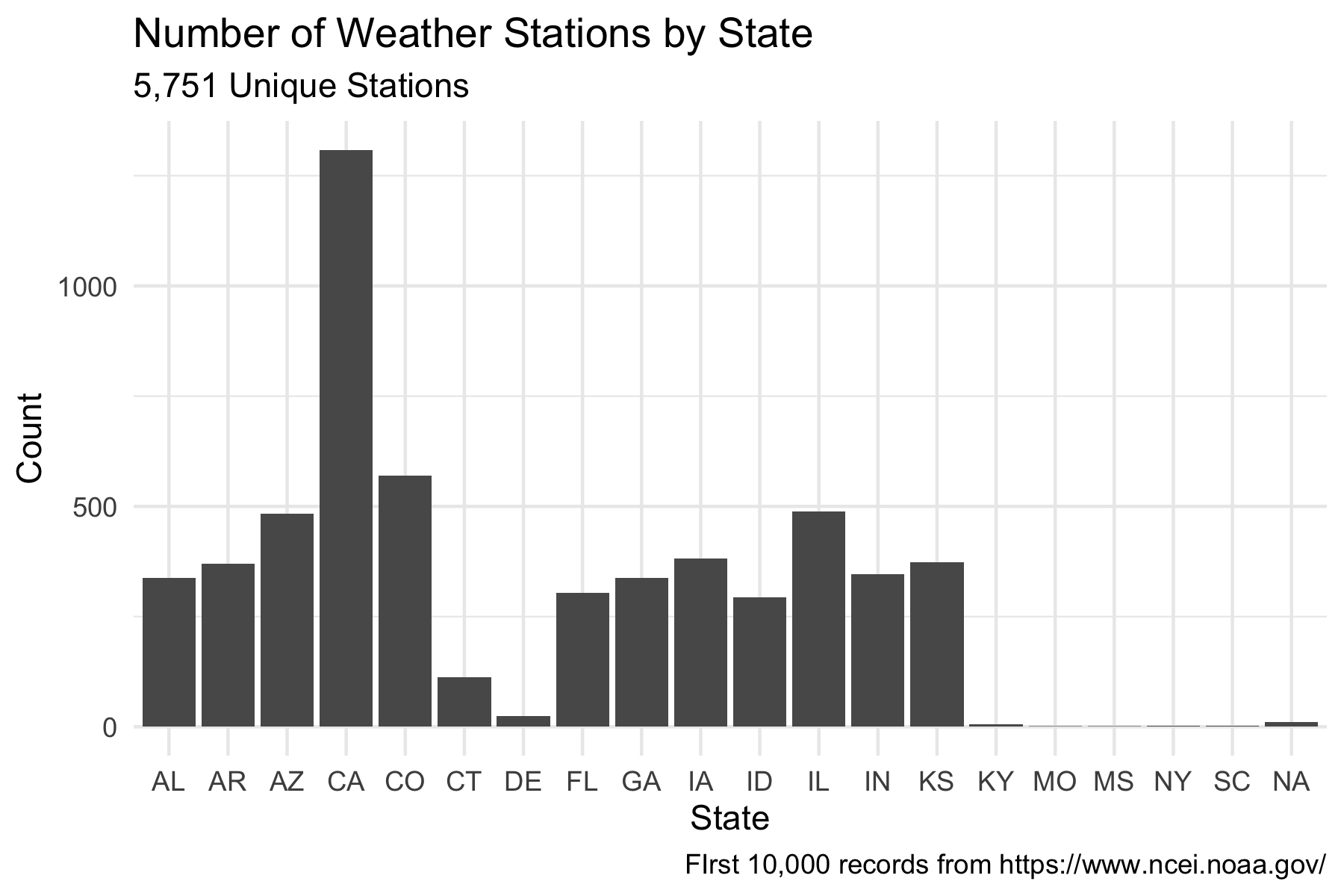
6.9.2 Example of Trefle.io API with Multiple Pages
This example demonstrates three different ways to paginate through an API to retrieve multiple pages of results:
- Using {httr2} with {purrr}.
- Using
httr2::req_perform_iterative()with a custom function to build the request for the next page. - Using
httr2::req_perform_iterative()andhttr2::iterate_with_offset()to automatically handle pagination via a numeric offset.
Depending on the API’s structure and complexity, one approach may be easier to implement than the others. All three approaches ultimately produce the same results.
Trefle.io is an API for providing access to information about plants. It aggregates data from other sites and user inputs to provide a centralized repository.
The API is in beta with sufficient Documentation to use the API.
- The API uses [pagination] to limit results to 30 items per page. To get more you need to request specific pages.
- There is a limit of 120 requests per minute
See Getting Started for instructions about getting a key and accessing the endpoint.
Load the libraries.
6.9.2.1 Using {purrr} to get multiple pages
The code starting with Listing 6.7 creates a vector of desired page numbers, builds a function to get a tibble of data from each page, and uses map() to get a list of the tibble for each page and then and list_rbind() to combine into a single tibble.
- Build a custom function to get one page of results as a tibble.
- Note the use of
(......)to wrap the request prior to the$dataso the entire left side of the$is evaluated.
- Note the use of
get_species <- \(page) {
  (
    request(trefle_URL) |>
    req_url_query(page = page) |>
    req_url_query(per_page = "20") |>
    req_url_query(token = key_get("API_KEY_TREFLE")) |>
    req_throttle(rate = 2) |>  # throttle (120 req/min limit)
    req_perform() |>
    resp_body_json()
    )$data |>
    tibble(data = _) |>
    unnest_wider(data)
}- Use
map()to get list of tibbles for all pages and thenlist_rbind()into one.
Rows: 600
Columns: 16
$ id                 <int> 77116, 109482, 227114, 128860, 11971, 51662, 230202…
$ common_name        <chr> "Evergreen oak", "Common nettle", "Barnyard grass",…
$ slug               <chr> "quercus-rotundifolia", "urtica-dioica", "dactylis-…
$ scientific_name    <chr> "Quercus rotundifolia", "Urtica dioica", "Dactylis …
$ year               <int> 1785, 1753, 1753, 1753, 1753, 1753, 1753, 1753, 175…
$ bibliography       <chr> "Encycl. 1: 723 (1785)", "Sp. Pl.: 984 (1753)", "Sp…
$ author             <chr> "Lam.", "L.", "L.", "L.", "L.", "L.", "L.", "L.", "…
$ status             <chr> "accepted", "accepted", "accepted", "accepted", "ac…
$ rank               <chr> "species", "species", "species", "species", "specie…
$ family_common_name <chr> NA, NA, NA, NA, "Aster family", NA, NA, NA, NA, NA,…
$ genus_id           <int> 3519, 5550, 10915, 6597, 250, 1872, 11051, 6311, 35…
$ image_url          <chr> "https://d2seqvvyy3b8p2.cloudfront.net/40ab8e7cdddb…
$ synonyms           <list> ["Quercus ilex var. oleoides", "Quercus ilex subva…
$ genus              <chr> "Quercus", "Urtica", "Dactylis", "Plantago", "Achil…
$ family             <chr> "Fagaceae", "Urticaceae", "Poaceae", "Plantaginacea…
$ links <list> ["/api/v1/species/quercus-rotundifolia", "/api/v1/…- Use the data for a plot.
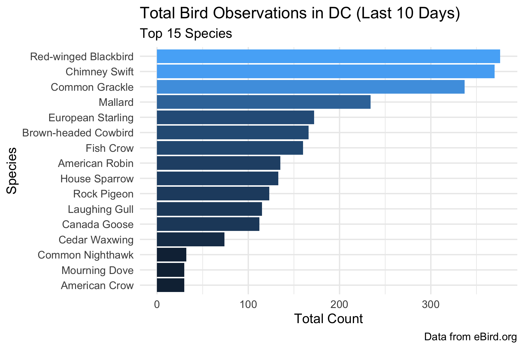
6.9.2.2 Using httr2::req_perform_iterative() withq a custom function to get multiple pages.
Listing 6.8 code uses the {httr2} functions req_perform_iterative() and a custom function to iterate the pages.
- Set the max_pages so you can troubleshoot on a low number and raise for the number you want when ready.
- Look at the example in the API documentation for pagination to find the links portion of the JSON response structure with the metadata for the the page status.
- Include a
Sys.sleep()to prevent exceeding the limits. - Add a safety check if there is no next page to stop
- If there is a next page, then update the request with the next page number and your key.
The req_perform_iterative() function returns a list of the page responses as output so you need to convert then to JSON and then tibbles and then combine into a single tibble.
- Build the initial request starting with page = 1
- Use
req_perform_iterative()to run the initial request and then use a custom function to extract the “next” url returned by each request to build the next request.
req_perform_iterative(
  req,
  next_req = function(resp, req) {             # build custom function
    resp_json <- resp_body_json(resp)
    next_url <- resp_json[["links"]][["next"]] # extract pagination link
    if (is.null(next_url)) return(NULL)       # stop when no next page
    req |>                                  # build and return the next request
      req_url(paste0("https://trefle.io", next_url)) |>
      req_url_query(token = key_get("API_KEY_TREFLE"))
  },
  max_reqs = max_pages, # safety cap so you don’t over-fetch
  progress = TRUE
) ->
plants_h- Use
map()convert responses from JSON into a tibble,unnest_wider(), and thenlist_ribind()into a single tibble.
Rows: 600
Columns: 16
$ id                 <int> 77116, 109482, 227114, 128860, 11971, 51662, 230202…
$ common_name        <chr> "Evergreen oak", "Common nettle", "Barnyard grass",…
$ slug               <chr> "quercus-rotundifolia", "urtica-dioica", "dactylis-…
$ scientific_name    <chr> "Quercus rotundifolia", "Urtica dioica", "Dactylis …
$ year               <int> 1785, 1753, 1753, 1753, 1753, 1753, 1753, 1753, 175…
$ bibliography       <chr> "Encycl. 1: 723 (1785)", "Sp. Pl.: 984 (1753)", "Sp…
$ author             <chr> "Lam.", "L.", "L.", "L.", "L.", "L.", "L.", "L.", "…
$ status             <chr> "accepted", "accepted", "accepted", "accepted", "ac…
$ rank               <chr> "species", "species", "species", "species", "specie…
$ family_common_name <chr> NA, NA, NA, NA, "Aster family", NA, NA, NA, NA, NA,…
$ genus_id           <int> 3519, 5550, 10915, 6597, 250, 1872, 11051, 6311, 35…
$ image_url          <chr> "https://d2seqvvyy3b8p2.cloudfront.net/40ab8e7cdddb…
$ synonyms           <list> ["Quercus ilex var. oleoides", "Quercus ilex subva…
$ genus              <chr> "Quercus", "Urtica", "Dactylis", "Plantago", "Achil…
$ family             <chr> "Fagaceae", "Urticaceae", "Poaceae", "Plantaginacea…
$ links              <list> ["/api/v1/species/quercus-rotundifolia", "/api/v1/…
6.9.2.3 Using httr2::req_perform_iterative() and httr2::iterate_with_offset() to get multiple pages.
Listing 6.9 code uses the {httr2} functions req_perform_iterative() and httr2::iterate_with_offset() to iterate the pages.
- Set the max_pages so you can troubleshoot on a low number and raise for the number you want when ready.
- With `
httr2::iterate_with_offset()you can try to let {httr2} figure out how to iterate if you set theparam-name = "page". - It is good to include a function for
resp_complete()as a safety check to avoid running out of pages.- Include a
req_throttle(rate = 5)to prevent exceeding the limits.
- Include a
The req_perform_iterative() function returns a list of the page responses as output so you need to convert then to JSON and then tibbles and then combine into a single tibble.
- Use {httr2} to build the initial request starting with page = 1
- Use
req_perform_iterative()withiterate_with_offset())to generate the list of responses for each page.
- Convert responses into tibble.
Rows: 600
Columns: 16
$ id                 <int> 77116, 109482, 227114, 128860, 11971, 51662, 230202…
$ common_name        <chr> "Evergreen oak", "Common nettle", "Barnyard grass",…
$ slug               <chr> "quercus-rotundifolia", "urtica-dioica", "dactylis-…
$ scientific_name    <chr> "Quercus rotundifolia", "Urtica dioica", "Dactylis …
$ year               <int> 1785, 1753, 1753, 1753, 1753, 1753, 1753, 1753, 175…
$ bibliography       <chr> "Encycl. 1: 723 (1785)", "Sp. Pl.: 984 (1753)", "Sp…
$ author             <chr> "Lam.", "L.", "L.", "L.", "L.", "L.", "L.", "L.", "…
$ status             <chr> "accepted", "accepted", "accepted", "accepted", "ac…
$ rank               <chr> "species", "species", "species", "species", "specie…
$ family_common_name <chr> NA, NA, NA, NA, "Aster family", NA, NA, NA, NA, NA,…
$ genus_id           <int> 3519, 5550, 10915, 6597, 250, 1872, 11051, 6311, 35…
$ image_url          <chr> "https://d2seqvvyy3b8p2.cloudfront.net/40ab8e7cdddb…
$ synonyms           <list> ["Quercus ilex var. oleoides", "Quercus ilex subva…
$ genus              <chr> "Quercus", "Urtica", "Dactylis", "Plantago", "Achil…
$ family             <chr> "Fagaceae", "Urticaceae", "Poaceae", "Plantaginacea…
$ links              <list> ["/api/v1/species/quercus-rotundifolia", "/api/v1/…
6.9.3 Example of the eBird API and Modifying the Endpoint
eBird is among the world’s largest biodiversity-related science projects, with more than 100 million bird sightings contributed annually by eBirders around the world. It is a collaborative enterprise with hundreds of partner organizations, thousands of regional experts, and hundreds of thousands of users. eBird is managed by the Cornell Lab of Ornithology.
The eBird 2.0 APIs provide multiple types of functionality.
- All APIs require a key you can get by signing up at Cornell Lab Account.
6.9.3.1 eBird API Endpoints and httr:req_url_path_append()
Instead of having one end point, the eBird APIs uses different end points for different types of requests such as recent sightings, geographic sightings, historical sightings, etc..
The data/obs documentation shows the multiple endpoints to cover different kinds of requests, how to construct an end point with specific parameters and then the query parameters specific to that end point that you can add to create a properly formed request to the API.
The end points have different limits on the number of records returned so you need to read the documentation carefully.
6.9.3.2 Historical Data
Let’s get “Historical observations on a date” for the DC region for the most recent 10 days.
The endpoint structure is https://api.ebird.org/v2/data/obs/{{regionCode}}/historic/{{y}}/{{m}}/{{d}}.
- Note that it includes the region code and the date as part of the end point.
We can use httr2::req_url_path_append() to build the endpoint piece by piece starting from the base URL - the part before the first end point parameter, {regionCode}.
- Once we have the endpoint constructed, we can use
req_url_query()to add the query parameters to it.
We can wrap the steps to build the endpoint and query inside a custom function and use purrr:::map(), or map2() if we want to vary more parameters than date, to get the data.
- Note there is no specified rate limit but 5 per second seems to be reasonable for
req_throttle().
Here is example code to implement the steps.
- Build the dates of interest as a sequence
- Define the Default Region and Date.
- Create the function to get the results for a region and date.
- Append each piece to the URL in turn.
get_bird <- function(region = "US-DC", date = "2025-07-01") {
  year <- str_sub(date, 1, 4)
  month <- str_sub(date, 6, 7)
  day <- str_sub(date, 9, 10)

 request("https://api.ebird.org/v2/data/obs/") |>
    req_url_path_append(region) |>
    req_url_path_append("historic") |>
    req_url_path_append(year) |>
    req_url_path_append(month) |>
    req_url_path_append(day) |>
    req_headers("X-eBirdApiToken" =  keyring::key_get("API_KEY_EBIRD")) |>
    req_throttle(rate = 5) |> # "requests per second"
    #req_url_query(detail = "full") |>
    req_perform() |>
    resp_body_json() |>
    tibble(data = _) |>
    unnest_wider(data)
}- Use
map()to process the sequence of dates with the custom function.- Convert each result to a tibble and combine all tibbles with
list_ribind().
- Convert each result to a tibble and combine all tibbles with
Rows: 737
Columns: 14
$ speciesCode     <chr> "chiswi", "rebwoo", "blujay", "fiscro", "carwre", "ame…
$ comName         <chr> "Chimney Swift", "Red-bellied Woodpecker", "Blue Jay",…
$ sciName         <chr> "Chaetura pelagica", "Melanerpes carolinus", "Cyanocit…
$ locId           <chr> "L2491807", "L2491807", "L2491807", "L2491807", "L2491…
$ locName         <chr> "Rock Creek Park--Reservation 630 (formerly Melvin C. …
$ obsDt           <chr> "2025-07-01 16:57", "2025-07-01 16:57", "2025-07-01 16…
$ howMany         <int> 3, 1, 1, 1, 1, 2, 1, 1, 1, 1, 2, 2, 1, 10, 1, 4, 1, 11…
$ lat             <dbl> 38.93882, 38.93882, 38.93882, 38.93882, 38.93882, 38.9…
$ lng             <dbl> -77.05877, -77.05877, -77.05877, -77.05877, -77.05877,…
$ obsValid        <lgl> TRUE, TRUE, TRUE, TRUE, TRUE, TRUE, TRUE, TRUE, TRUE, …
$ obsReviewed     <lgl> FALSE, FALSE, FALSE, FALSE, FALSE, FALSE, FALSE, FALSE…
$ locationPrivate <lgl> FALSE, FALSE, FALSE, FALSE, FALSE, FALSE, FALSE, FALSE…
$ subId           <chr> "S256031072", "S256031072", "S256031072", "S256031072"…
$ exoticCategory  <chr> NA, NA, NA, NA, NA, NA, "N", NA, NA, NA, NA, NA, NA, N…
Create a variety of plots.
Given the number of species and locations, these focus on the “top” species or locations in terms of total counts.
Total Bird Observations in DC (Last 10 Days)
# Summarize total count by species
bird_data  |>
  group_by(comName) |>
  summarise(total_count = sum(howMany, na.rm = TRUE)) ->
  species_counts

species_counts |>
  slice_max(order_by = total_count, n = 15) |>
ggplot(aes(
       x = fct_reorder(comName, total_count),
       y = total_count,
       fill = total_count
     )) +
  geom_col(show.legend = FALSE) +
  coord_flip() +
  labs(
    title = "Total Bird Observations in DC (Last 10 Days)",
    subtitle = "Top 15 Species",
    caption = "Data from eBird.org",
    x = "Species",
    y = "Total Count"
  ) +
  theme_minimal() ->
p1- Daily Bird Observations in DC (Last 10 Days)
# Ensure observation date is Date class
bird_data <- bird_data |>
  mutate(obsDate = ymd_hm(obsDt))  # lubridate ymd() parses "YYYY-MM-DD"

# Summarize counts per species per day
daily_counts <- bird_data |>
  group_by(obsDate, comName) |>
  summarise(daily_count = sum(howMany, na.rm = TRUE), .groups = "drop")

# Order species by total counts across all days
species_order <- daily_counts |>
  group_by(comName) |>
  summarise(total_count = sum(daily_count), .groups = "drop") |>
  arrange(desc(total_count)) |>
  pull(comName)

daily_counts <- daily_counts |>
  mutate(commonName = fct_relevel(comName, species_order))

# Line plot
daily_counts |>
  slice_max(order_by = daily_count, n = 15) |>
ggplot(aes(x = obsDate, y = daily_count,
                         color = comName, group = comName)) +
  geom_line(linewidth = 1) +
  geom_point(size = 2) +
  labs(
    title = "Daily Bird Observations in DC (Last 10 Days)",
    caption = "Data from eBird.org",
    subtitle = "Top 15 Species",
    x = "Date",
    y = "Count",
    color = "Species"
  ) +
  theme_minimal() +
  theme(legend.position = "right") ->
p2- Distribution of Total Bird Counts by Top 10 Locations in DC (Last 10 Days)
Combine plots into one line of output using quarto layout.
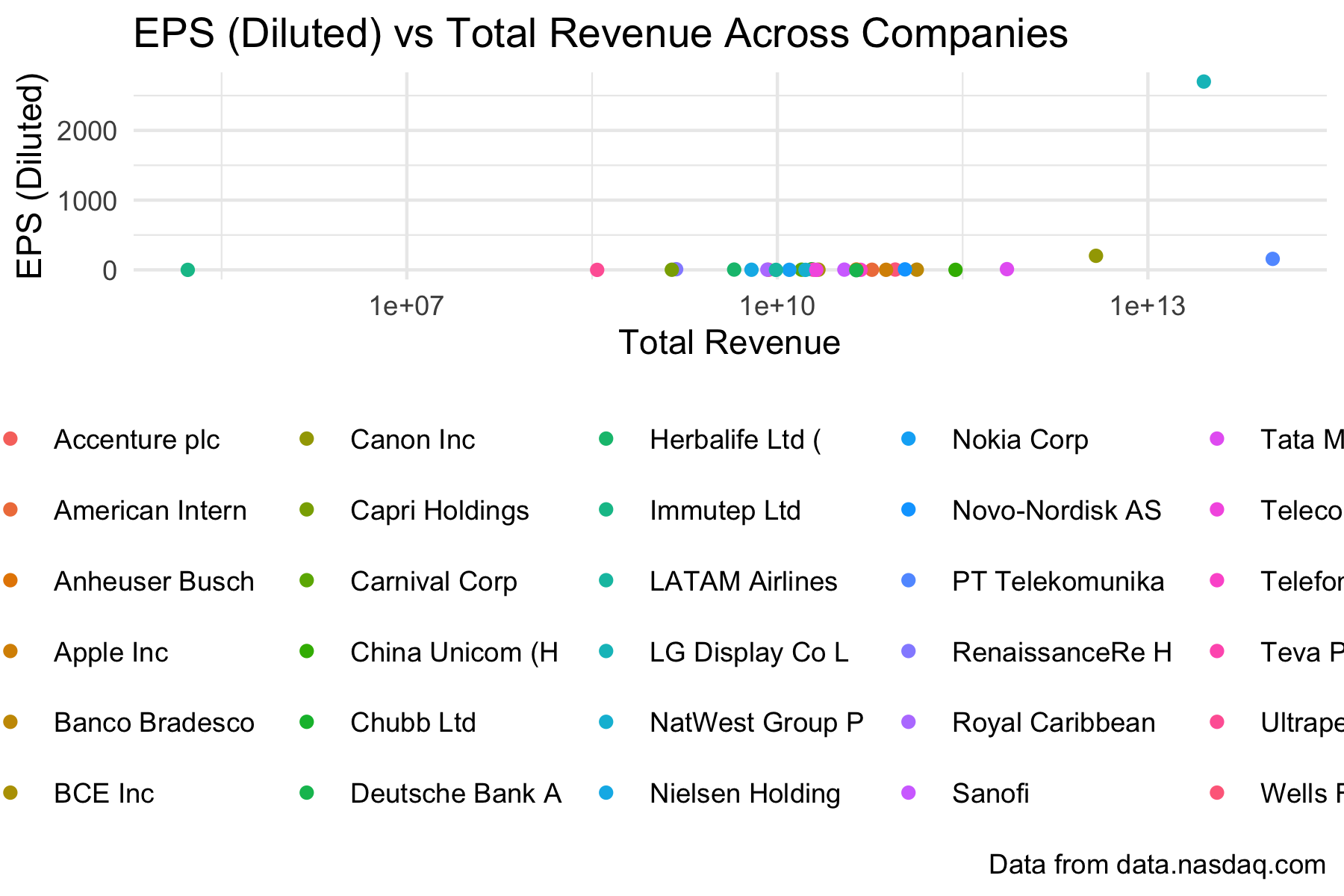
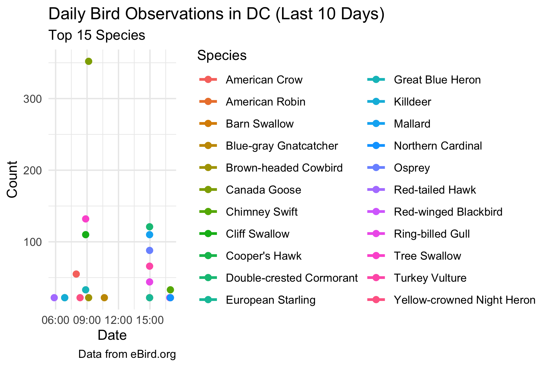
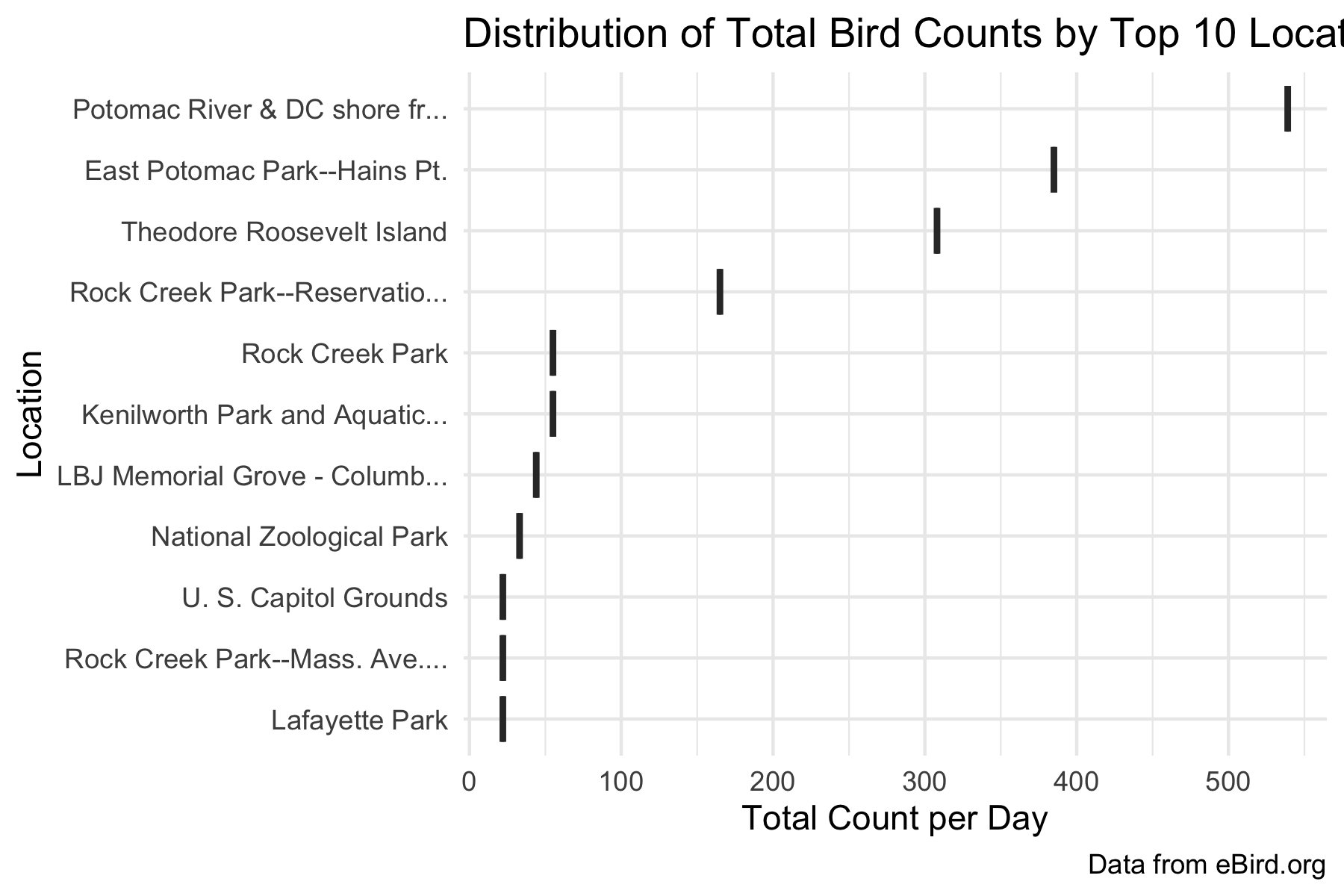
This is an example where the {httr2} helper functions will not help much as they are about paginating on query indexes and pages for one endpoint, and not rebuilding endpoints.
The {purrr}-based strategy seems to be the cleaner strategy for this API.
6.9.4 Other Examples APIs
6.9.5 {NasdaqDataLink} R Package
Nasdaq is a global financial services company that supports the buying and selling of securities among many other services.
- The Nasdaq Data Link has a large collection of data for use by institutional investors, fintech companies and individual users.
- Nasdaq provides the {NasdaqDataLink} R Package to access the API.
Install the package from CRAN using the console and load it.
You need an account and an API key which is available through the Getting Started page.
- Once you have your key, use {keyring} to set as “API_KEY_NASDAQ” and then get for queries.
Let the package know your key:
Access the data product of interest. See options at DATA ORGANIZATION, ACCESS OPTIONS AND AUTHENTICATION
- The following accesses the Mergent Global Fundamentals Data Table. Set
paginate = TRUEto allow for up to 1M records.
Rows: 30,769
Columns: 5
$ compnumber <dbl> 2438, 2438, 2438, 2438, 2438, 2438, 2438, 17630, 17630, 176…
$ shortname  <chr> "Deutsche Bank AG", "Deutsche Bank AG", "Deutsche Bank AG",…
$ reportdate <date> 2011-06-30, 2011-09-30, 2012-06-30, 2012-09-30, 2013-06-30…
$ indicator  <chr> "Accrued Expenses Turnover", "Accrued Expenses Turnover", "…
$ amount     <dbl> 1.048195e+01, 8.161754e+00, 1.078821e+01, 9.437545e+00, 8.7…
See the unique indicators.
 [1] "Accounts Payable"
 [2] "Accounts Payable Turnover"
 [3] "Accrued Expenses Turnover"
 [4] "Calculated Tax Rate"
 [5] "Cash & Equivalents Turnover"
 [6] "Cash and Equivalents"
 [7] "Cash Flow Per Share"
 [8] "Cash From Financing"
 [9] "Cash From Investing"
[10] "Cash From Operations"
[11] "Cash, Beginning of Year"
[12] "Cash, End of Year"
[13] "Current Assets"
[14] "Current Liabilities"
[15] "Current Ratio"
[16] "Direct Expenses"
[17] "EBITDA"
[18] "EBITDA Margin"
[19] "EPS - Net Income - Basic"
[20] "EPS - Net Income - Diluted"
[21] "Free Cash Flow Per Share"
[22] "Gross Margin"
[23] "Interest Coverage"
[24] "Inventories"
[25] "Inventory Turnover"
[26] "Long Term Debt"
[27] "Long Term Debt to Equity"
[28] "Net Current Assets as % of Total Assets"
[29] "Net Income"
[30] "Net Income Per Employee"
[31] "Net Margin"
[32] "Operating Income"
[33] "Operating Margin"
[34] "PP&E Turnover"
[35] "Quick Ratio"
[36] "Receivables"
[37] "Receivables Turnover"
[38] "Return on Assets"
[39] "Return on Equity"
[40] "Return on Investment"
[41] "Revenue Per Employee"
[42] "Revenue Per Share"
[43] "Revenue to Assets"
[44] "Shares Outstanding"
[45] "Stockholders' Equity"
[46] "Total Asset Turnover"
[47] "Total Assets"
[48] "Total Assets Per Share"
[49] "Total Debt to Equity"
[50] "Total Liabilities"
[51] "Total Revenue"
[52] "Weighted Average Shares Outstanding - Basic"
[53] "Weighted Average Shares Outstanding - Diluted"
Since not all companies use the same indicators, see which ones are the most common.
# A tibble: 53 × 2
   indicator                    n
   <chr>                    <int>
 1 Total Assets Per Share      55
 2 Shares Outstanding          54
 3 EPS - Net Income - Basic    53
 4 Net Income                  52
 5 Net Margin                  52
 6 Total Revenue               52
 7 Cash and Equivalents        51
 8 Cash, End of Year           51
 9 EBITDA                      51
10 EBITDA Margin               51
# ℹ 43 more rows
Let’s filter to two common indicators, Earnings per Share and Revenue and plot the companies with those indicators based on their latest report.
my_df |>
  filter(indicator %in% c("EPS - Net Income - Basic", "Total Revenue")) |>
  distinct(compnumber, reportdate, indicator, .keep_all = TRUE) |>
  group_by(compnumber) |>
  filter(reportdate == max(reportdate)) |>
  ungroup() |>
  mutate(shortname = str_sub(shortname, end = 15)) |>
  pivot_wider(
    names_from = indicator,
    values_from = amount
  ) |>
  filter(!is.na(`Total Revenue`), !is.na(`EPS - Net Income - Basic`)) |>
  ggplot(aes(x = `Total Revenue`, y = `EPS - Net Income - Basic`, color = shortname)) +
  geom_point() +
  labs(
    title = "EPS (Diluted) vs Total Revenue Across Companies",
    caption = "Data from data.nasdaq.com",
    x = "Total Revenue",
    y = "EPS (Diluted)",
    color = NULL
  ) +
  theme_minimal() +
  theme(legend.position = "bottom") +
  scale_x_log10()
6.9.6 Examples Using the USASpending API
6.9.6.1 Introduction
USA Spending is the US government’s website for providing open access to US government financial data. The website allows individual downloads and bulk downloads.
There is also a USASPending API for programmatic access for simple filters and advanced filters to help you get the exact data you want in a repeatable manner.
There are many endpoints and each endpoint has multiple objects you can use to establish filters for your request.
This document has examples for using R with {tidyverse} and {httr2} packages to get data from USASpending using their API. The examples below demonstrate how to formulate and use
- a GET request for simple filtering,
- a POST request for advanced filtering, and,
- a POST request to create a Zip file for download from USASpending.
Each of the filters in the below are just examples and you will have to tailor requests to match the exact type of data you are seeking.
Load libraries
6.9.6.2 Simple Filtering with a GET Request
Multiple USA Spending end points all for using a GET request for simple filters.
See USASpending
The parameters of the end point must be in the URL before the ? to get to the right end-point. This includes the agency ID
- Create the request
- Test the request query.
$fiscal_year
[1] 2026

$latest_action_date
[1] "2026-09-30T00:00:00"

$toptier_code
[1] "012"

$transaction_count
[1] 1395426

$obligations
[1] 125137502383

$messages
list()- Add the query attribute for fiscal year.
- Build a function to get data for an end point and a year.
$fiscal_year
[1] 2018

$latest_action_date
[1] "2018-09-30T00:00:00"

$toptier_code
[1] "012"

$transaction_count
[1] 4014251

$obligations
[1] 122523530633

$messages
list()- Build input data
- Use
map2()to get the results.
- Convert to tibble and unnest to a data frame.
Rows: 5
Columns: 6
$ fiscal_year        <int> 2018, 2019, 2020, 2021, 2022
$ latest_action_date <chr> "2018-09-30T00:00:00", "2019-09-30T00:00:00", "2020…
$ toptier_code       <chr> "012", "012", "012", "012", "012"
$ transaction_count  <int> 4014251, 4159008, 4692410, 6372946, 3272895
$ obligations        <dbl> 122523530633, 122788916598, 168094147259, 224814046…
$ messages           <lgl> NA, NA, NA, NA, NA
6.9.6.3 POST request for Advanced Filtering
for endpoint ‘[/api/v2/search/spending_by_award/]’
- Create the request object
- Load libraries
- Establish the request using the end point URL.
<httr2_request>
GET https://api.usaspending.gov/api/v2/search/spending_by_award/
Body: empty- Request a Single Page
Build the body of the request as a named list.
You have to be careful to get the main body “objects” in the top level list and any sub elements for the objects as their own vector or list within the main object element, e.g., filters and time_period.
request_data <- list(
  "subawards" = "false",
  "limit" = 100,
  # "page" = 1,
  "filters" = list(
    "award_type_codes" = c("A", "B", "C", "D"),
    "agency" = c(1, 2),
    "time_period" = list(
      list(
        "start_date" = "2018-10-01",
        "end_date" = "2019-09-30"
      )
    ) # end of time period object list
  ), # end of Filters list
  "fields" = c(
    "Award ID",
    "Recipient Name",
    "Start Date",
    "End Date",
    "Award Amount",
    "Awarding Agency",
    "Awarding Sub Agency",
    "Contract Award Type",
    "Award Type",
    "Funding Agency",
    "Funding Sub Agency"
  )
)- Convert to JSON and visually compare your named list as a JSON string to the example on the webpage.
{"subawards":"false","limit":100,"filters":{"award_type_codes":["A","B","C","D"],"agency":[1,2],"time_period":[{"start_date":"2018-10-01","end_date":"2019-09-30"}]},"fields":["Award ID","Recipient Name","Start Date","End Date","Award Amount","Awarding Agency","Awarding Sub Agency","Contract Award Type","Award Type","Funding Agency","Funding Sub Agency"]} - Test running as a named list.
- Test running the encoded JSON as a raw string
- Test converting the output from the query into a data frame.
# A tibble: 100 × 15
   internal_id `Award ID` `Recipient Name`               `Start Date` `End Date`
         <int> <chr>      <chr>                          <chr>        <chr>
 1   350880934 ZZ65       ATT MOBILITY LLC               2016-12-30   2018-12-31
 2   350880905 ZZ62       COOPER BUILDING SERVICES, LLC  2018-01-24   2019-04-26
 3   350880893 ZZ61       ATT MOBILITY LLC               2016-12-30   2018-12-31
 4   350880892 ZZ61       COOPER BUILDING SERVICES, LLC  2018-01-24   2020-04-27
 5   350880102 ZZ01       TETRA TECH/MEAD AND HUNT JOIN… 2017-07-19   2024-03-11
 6   350880095 ZZ01       RICOH USA INC                  2016-08-19   2021-09-14
 7   350878352 ZX10       CACI IDT, LLC                  2018-01-31   2019-01-02
 8   350878226 ZX04       WILDFLOWER INTERNATIONAL, LTD. 2017-05-23   2017-05-31
 9   350878118 ZX01       CH2M HILL - HDR JV             2017-09-12   2021-07-30
10   350878086 ZX01       NATIONAL INDUSTRIES FOR THE B… 2017-09-06   2018-02-28
# ℹ 90 more rows
# ℹ 10 more variables: `Award Amount` <dbl>, `Awarding Agency` <chr>,
#   `Awarding Sub Agency` <chr>, `Contract Award Type` <chr>,
#   `Award Type` <lgl>, `Funding Agency` <chr>, `Funding Sub Agency` <chr>,
#   awarding_agency_id <int>, agency_slug <chr>, generated_internal_id <chr>
6.9.6.4 Use {purrr} to get Multiple Pages
The limit is 100 results per page. However, you can run multiple queries using purrr::map().
Build a function to process a request for each page.
- If you have multiple arguments you want to change each time, consider converting the function to
map2()orpmap(). - The following assumes the
reqargument already exists for this endpoint.
get_data <- function(req = req, page = 1) {
  request_data <- list(
    "subawards" = "false",
    "limit" = 100, # the max for a page
    "page" = page,
    "filters" = list(
      "award_type_codes" = c("A", "B", "C", "D"),
      "agency" = c(1, 2),
      "time_period" = list(
        list(
          "start_date" = "2018-10-01",
          "end_date" = "2019-09-30"
        )
      ) # end of time period object list
    ), # end of Filters list
    "fields" = c(
      "Award ID",
      "Recipient Name",
      "Start Date",
      "End Date",
      "Award Amount",
      "Awarding Agency",
      "Awarding Sub Agency",
      "Contract Award Type",
      "Award Type",
      "Funding Agency",
      "Funding Sub Agency"
    )
  )
  # use the req to execute the body where req_body_json will encode
  # the named list into a valid JSON string
  req |>
    req_body_json(data = request_data) |>
    req_perform() |>
    resp_body_json() -> tempp

  # process the return object results to get a data frame
  tempp$results |>
    tibble(data = _) |>
    unnest_wider(data)
}- Test the function
# A tibble: 100 × 15
   internal_id `Award ID` `Recipient Name`               `Start Date` `End Date`
         <int> <chr>      <chr>                          <chr>        <chr>
 1   350880934 ZZ65       ATT MOBILITY LLC               2016-12-30   2018-12-31
 2   350880905 ZZ62       COOPER BUILDING SERVICES, LLC  2018-01-24   2019-04-26
 3   350880893 ZZ61       ATT MOBILITY LLC               2016-12-30   2018-12-31
 4   350880892 ZZ61       COOPER BUILDING SERVICES, LLC  2018-01-24   2020-04-27
 5   350880102 ZZ01       TETRA TECH/MEAD AND HUNT JOIN… 2017-07-19   2024-03-11
 6   350880095 ZZ01       RICOH USA INC                  2016-08-19   2021-09-14
 7   350878352 ZX10       CACI IDT, LLC                  2018-01-31   2019-01-02
 8   350878226 ZX04       WILDFLOWER INTERNATIONAL, LTD. 2017-05-23   2017-05-31
 9   350878118 ZX01       CH2M HILL - HDR JV             2017-09-12   2021-07-30
10   350878086 ZX01       NATIONAL INDUSTRIES FOR THE B… 2017-09-06   2018-02-28
# ℹ 90 more rows
# ℹ 10 more variables: `Award Amount` <dbl>, `Awarding Agency` <chr>,
#   `Awarding Sub Agency` <chr>, `Contract Award Type` <chr>,
#   `Award Type` <lgl>, `Funding Agency` <chr>, `Funding Sub Agency` <chr>,
# awarding_agency_id <int>, agency_slug <chr>, generated_internal_id <chr>- Create a vector for the pages of interest.
- Run the multi-page bulk request.
- Each request returns a data frame so use
purrrr:list_rbind()to collapse them to a single data frame.
[1] 1000- An equivalent request using HTTR for a single POST request
# A tibble: 100 × 15
   internal_id `Award ID` `Recipient Name`               `Start Date` `End Date`
         <int> <chr>      <chr>                          <chr>        <chr>
 1   350880934 ZZ65       ATT MOBILITY LLC               2016-12-30   2018-12-31
 2   350880905 ZZ62       COOPER BUILDING SERVICES, LLC  2018-01-24   2019-04-26
 3   350880893 ZZ61       ATT MOBILITY LLC               2016-12-30   2018-12-31
 4   350880892 ZZ61       COOPER BUILDING SERVICES, LLC  2018-01-24   2020-04-27
 5   350880102 ZZ01       TETRA TECH/MEAD AND HUNT JOIN… 2017-07-19   2024-03-11
 6   350880095 ZZ01       RICOH USA INC                  2016-08-19   2021-09-14
 7   350878352 ZX10       CACI IDT, LLC                  2018-01-31   2019-01-02
 8   350878226 ZX04       WILDFLOWER INTERNATIONAL, LTD. 2017-05-23   2017-05-31
 9   350878118 ZX01       CH2M HILL - HDR JV             2017-09-12   2021-07-30
10   350878086 ZX01       NATIONAL INDUSTRIES FOR THE B… 2017-09-06   2018-02-28
# ℹ 90 more rows
# ℹ 10 more variables: `Award Amount` <dbl>, `Awarding Agency` <chr>,
#   `Awarding Sub Agency` <chr>, `Contract Award Type` <chr>,
#   `Award Type` <lgl>, `Funding Agency` <chr>, `Funding Sub Agency` <chr>,
#   awarding_agency_id <int>, agency_slug <chr>, generated_internal_id <chr>
6.9.6.5 Dowload Zip file of CSVs for Awards
USASpending also allows you to generate a request for bulkdownload as a Zip file of multiple CSVs.
See Award Download ‘[/api/v2/download/awards/]’ for details.
- Create the post request to identify the desired data.
<httr2_request>
GET https://api.usaspending.gov/api/v2/download/awards/
Body: empty
request_data <- list(
"limit" = 1000,
"filters" = list(
"agencies" = list(
list(
"type" = "awarding",
"tier" = "toptier",
"name" = "Department of Agriculture"
)
),
"keywords" = c("Defense", "Interior")
),
"columns" = c(
"assistance_award_unique_key",
"award_id_fain",
"award_id_uri",
"sai_number",
"total_funding_amount"
)
)- Create a JSON version to compare to the website example.
{"limit":1000,"filters":{"agencies":[{"type":"awarding","tier":"toptier","name":"Department of Agriculture"}],"keywords":["Defense","Interior"]},"columns":["assistance_award_unique_key","award_id_fain","award_id_uri","sai_number","total_funding_amount"]} - Submit the POST query to the API and save the return.
- Use the response to identify the URL for the zip files.
- You have to manually download the files as vroom will not read zip files from a URL.
- Download and move into the desired data directory and unzip.
[1] "https://files.usaspending.gov/generated_downloads/PrimeAwardSummariesAndSubawards_2026-07-14_H15M19S18839483.zip"
Note
The following section will have to be tailored to the results of the download and the associated directory with the unzipped files.
Multiple files may be returned in the zip file, even if an individual file has no records.
- Edit the path.
- It adds the path and looks for the files in directory created by unzipping the downloaded files.
- It gets the file info, filters out the files with size 0, and converts row names to a variable.
- It then it reads in each file and (assuming they have consistent columns), combines into a single data frame.
6.10 Summary for Getting Data Using APIs
Organizations use APIs to provide access to select data in a structured way that allows them control over who is accessing and how much, while allowing the user to customize which data they want.
If there is an R package to wrap the API, that often saves you time and effort. If there is not one, you can work with the {httr} package and the API documentation to access the data.
Given the complexity of data sets, the semi-structured JSON format is convenient for data exchange with APIs. Multiple R packages provide functions to help you manipulate the output from APIs to support your analysis.
6.11 Manipulating Deeply Nested Data
Data from many APIs, often called “wild-caught JSON”, can be in deeply nested data structures as organizations try to maximize the efficiency of their data structures for storage and transfer rather than analysis.
“Rectangling” is the “art and craft” of taking a “wild” deeply-nested list and “taming” it into a tidy data set of rows and columns for the data of interest.
The goal of the {tidyr} package Wickham et al. (2023) is to help users convert data from a variety of sources into “tidy” data amenable for analysis and modeling.
Functions in the {tidyr} package that are particularly useful for rectangling include:
unnest_longer(): takes each element of a list-column and makes a new row.unnest_wider(): takes each element of a list-column and makes a new column.unnest_auto(): guesses whether you wantunnest_longer()orunnest_wider().hoist(): is similar tounnest_wider()but only plucks out selected components, and can reach down multiple levels.
Many data rectangling problems can be solved by combining these functions with a splash of {dplyr} (largely eliminating prior approaches that combined mutate() with multiple purrr::map()s).
Let’s load several packages we need for this section.
The {repurrrsive} package Bryan (2023) provides a number deeply-nested lists (most originally captured from web APIs).
Install the {repurrrsive} package using the console and load it.
6.11.1 Initial Example: GitHub Users
We’ll start with gh_users, an unnamed list with data on six GitHub users.
- Each GitHub user is a named list with 30 identical elements, each of which is an atomic vector of length one.
- These elements are what we want to become columns in a data frame.
To begin, let’s use tibble() to convert the gh_users list into a data frame where the list is now a list-column in the data frame.
Rows: 6
Columns: 1
$ user <list> ["gaborcsardi", 660288, "https://avatars.githubusercontent.com/u…- This seems a bit counter-intuitive: Why is the first step in making a list simpler to make it more complicated?
- Because, converting into a data frame creates a big advantage for us; multiple vectors are now tracked together in a single data frame with a consistent structure.
- We have multiple tools in Tidyverse for working with data frames.
Let’s use unnest_wider() to turn each element of the list column into a new column:
- Look at help for
unnest_wider()to see there are two mandatory arguments:dataandcol.
We have one list column in our data frame so unnest_wider() will flatten the row for each user into new columns in our data frame in one step.
# A tibble: 6 × 30
  login     id avatar_url gravatar_id url   html_url followers_url following_url
  <chr>  <int> <chr>      <chr>       <chr> <chr>    <chr>         <chr>
1 gabo… 6.60e5 https://a… ""          http… https:/… https://api.… https://api.…
2 jenn… 5.99e5 https://a… ""          http… https:/… https://api.… https://api.…
3 jtle… 1.57e6 https://a… ""          http… https:/… https://api.… https://api.…
4 juli… 1.25e7 https://a… ""          http… https:/… https://api.… https://api.…
5 leep… 3.51e6 https://a… ""          http… https:/… https://api.… https://api.…
6 masa… 8.36e6 https://a… ""          http… https:/… https://api.… https://api.…
# ℹ 22 more variables: gists_url <chr>, starred_url <chr>,
#   subscriptions_url <chr>, organizations_url <chr>, repos_url <chr>,
#   events_url <chr>, received_events_url <chr>, type <chr>, site_admin <lgl>,
#   name <chr>, company <chr>, blog <chr>, location <chr>, email <chr>,
#   hireable <lgl>, bio <chr>, public_repos <int>, public_gists <int>,
#   followers <int>, following <int>, created_at <chr>, updated_at <chr>
However, we are only interested in a few elements of the user lists so we don’t need to flatten all of the elements into the data frame.
We can instead use tidyr::hoist() to pull out the elements of interest using the same syntax as purrr::pluck()and leave the rest in the list column.
Let’s hoist the variables login,html_url,and followers, from column user.
# A tibble: 6 × 4
  login       url                            followers user
  <chr>       <chr>                              <int> <list>
1 gaborcsardi https://github.com/gaborcsardi       303 <named list [27]>
2 jennybc     https://github.com/jennybc           780 <named list [27]>
3 jtleek      https://github.com/jtleek           3958 <named list [27]>
4 juliasilge  https://github.com/juliasilge        115 <named list [27]>
5 leeper      https://github.com/leeper            213 <named list [27]>
6 masalmon https://github.com/masalmon 34 <named list [27]>- Notice it leaves the other 27 elements in the list
user. hoist()removes the named components from the user list-column, so you can think of it as moving components out of the “inner list” into the “top-level data frame”.
6.11.2 A More Complicated Example: gh_repos
The data set gh_repos is an un-named list with 6 elements.
- Each element is itself a list of 26 or 30 repos for a specific GitHub user.
- Each repo is a list of at least 68 elements with data about each repo such as name, owner (another list), fork status, and creation date.
Let’s use map_*() functions to confirm the structure.
[1] 30 30 30 26 30 30[[1]]
[1] 68 68 68 68 68 68 68 68 68 68 68 68 68 68 68 68 68 68 68 68 68 68 68 68 68
[26] 68 68 68 68 68
[[2]]
[1] 68 68 68 68 68 68 68 68 68 68 68 68 68 68 68 68 68 68 68 68 68 68 68 68 68
[26] 68 68 68 68 68
[[3]]
[1] 68 68 68 68 68 68 68 68 68 68 68 68 68 68 68 68 68 68 68 68 68 68 68 68 68
[26] 68 68 68 68 68
[[4]]
[1] 68 68 68 68 68 68 68 68 68 68 68 68 68 68 68 68 68 68 68 68 68 68 68 68 68
[26] 68
[[5]]
[1] 68 68 68 68 68 68 68 68 68 68 68 68 68 68 68 68 68 68 68 68 68 68 68 68 68
[26] 68 68 68 68 68
[[6]]
[1] 68 68 68 68 68 68 68 68 68 68 68 68 68 68 68 68 68 68 68 68 68 68 68 68 68
[26] 68 68 68 68 68
Tip
Use care in calling functions such as str() or glimpse() on deeply nested objects as they will go through each layer.
When using RStudio, Base R utils::View() will allow you to examine the data interactively to see the structure and contents.
Let’s convert gh_repos into a tibble like before.
[1] 30 30 30 26 30 30The elements of user are a list of repositories that belong to each user.
- Consider them as “observations”, so they could become new rows.
Use unnest_longer() to create rows (rather than unnest_wider() which creates columns).
- This is similar to {tidyr}’s
pivot_longer()andpivot_wider().
# A tibble: 6 × 1
  repo
  <list>
1 <named list [68]>
2 <named list [68]>
3 <named list [68]>
4 <named list [68]>
5 <named list [68]>
6 <named list [68]>[1] 176[1] 176We have removed one layer of the list if you will, so, we now have a list-column where each of the 176 repos is now a row.
- Each of these rows/observations is a list with 68 potential columns.
- Not all 68 plus columns are of length 1. Each repo has an
ownerelement which is a list with 17 elements. - Base R
unlist()can convert the list to a named vector.
                                               login
                                       "gaborcsardi"
                                                  id
                                            "660288"
                                          avatar_url
"https://avatars.githubusercontent.com/u/660288?v=3"
                                         gravatar_id
"" We can now use unnest_wider() or hoist() as before on this list column to get all or just specific element as columns in a data frame.
# A tibble: 10 × 5
   login       name                 watchers homepage               repo
   <chr>       <chr>                   <int> <chr>                  <list>
 1 gaborcsardi pingr                       2 ""                     <named list>
 2 jtleek      genstats_site               7  <NA>                  <named list>
 3 masalmon    convertagd                  0 ""                     <named list>
 4 juliasilge  juliasilge.github.io        0 "http://juliasilge.co… <named list>
 5 juliasilge  r-travis                    0  <NA>                  <named list>
 6 leeper      drat                        0  <NA>                  <named list>
 7 leeper      designcourse                1  <NA>                  <named list>
 8 masalmon    openaq_figures              1 ""                     <named list>
 9 leeper      GREA                        0 ""                     <named list>
10 leeper dataverse-1 0 "http://dataverse.org" <named list>- Note the use of
c("owner", "login"): this allowed us to reach two levels deep into of each list. - An alternative approach would be to pull out just
ownerand then put each of the 17 elements of it in a column:
# A tibble: 176 × 18
   login           id avatar_url        gravatar_id url   html_url followers_url
   <chr>        <int> <chr>             <chr>       <chr> <chr>    <chr>
 1 gaborcsardi 660288 https://avatars.… ""          http… https:/… https://api.…
 2 gaborcsardi 660288 https://avatars.… ""          http… https:/… https://api.…
 3 gaborcsardi 660288 https://avatars.… ""          http… https:/… https://api.…
 4 gaborcsardi 660288 https://avatars.… ""          http… https:/… https://api.…
 5 gaborcsardi 660288 https://avatars.… ""          http… https:/… https://api.…
 6 gaborcsardi 660288 https://avatars.… ""          http… https:/… https://api.…
 7 gaborcsardi 660288 https://avatars.… ""          http… https:/… https://api.…
 8 gaborcsardi 660288 https://avatars.… ""          http… https:/… https://api.…
 9 gaborcsardi 660288 https://avatars.… ""          http… https:/… https://api.…
10 gaborcsardi 660288 https://avatars.… ""          http… https:/… https://api.…
# ℹ 166 more rows
# ℹ 11 more variables: following_url <chr>, gists_url <chr>, starred_url <chr>,
#   subscriptions_url <chr>, organizations_url <chr>, repos_url <chr>,
#   events_url <chr>, received_events_url <chr>, type <chr>, site_admin <lgl>,
#   repo <list>
Instead of looking at the list and thinking about whether it needs to become rows or columns, you can try unnest_auto().
- It uses a few heuristics to figure out whether
unnest_longer()orunnest_wider()is appropriate, and tells you about its reasoning. - This is convenient for exploration but it is not advised to rely on it in long-term code.
unnest_auto()has the undesirable property that it will always succeed; that means if your data structure changes,unnest_auto()will continue to work, but might give very different output that causes cryptic failures from downstream functions.
6.11.3 An Even More Complicated Example: Game of Thrones Characters
The got_chars data set has a similar structure to gh_users; it’s a list of named lists, where each element of the inner list describes some attribute of a GoT character.
We start in the same way, first by creating a data frame and then by unnesting each component into a column.
Rows: 30
Columns: 18
$ url         <chr> "https://www.anapioficeandfire.com/api/characters/1022", "…
$ id          <int> 1022, 1052, 1074, 1109, 1166, 1267, 1295, 130, 1303, 1319,…
$ name        <chr> "Theon Greyjoy", "Tyrion Lannister", "Victarion Greyjoy", …
$ gender      <chr> "Male", "Male", "Male", "Male", "Male", "Male", "Male", "F…
$ culture     <chr> "Ironborn", "", "Ironborn", "", "Norvoshi", "", "", "Dorni…
$ born        <chr> "In 278 AC or 279 AC, at Pyke", "In 273 AC, at Casterly Ro…
$ died        <chr> "", "", "", "In 297 AC, at Haunted Forest", "", "In 299 AC…
$ alive       <lgl> TRUE, TRUE, TRUE, FALSE, TRUE, FALSE, FALSE, TRUE, TRUE, T…
$ titles      <list> <"Prince of Winterfell", "Lord of the Iron Islands (by la…
$ aliases     <list> <"Prince of Fools", "Theon Turncloak", "Reek", "Theon Kin…
$ father      <chr> "", "", "", "", "", "", "", "", "", "", "", "", "", "", ""…
$ mother      <chr> "", "", "", "", "", "", "", "", "", "", "", "", "", "", ""…
$ spouse      <chr> "", "https://www.anapioficeandfire.com/api/characters/2044…
$ allegiances <list> "House Greyjoy of Pyke", "House Lannister of Casterly Roc…
$ books       <list> <"A Game of Thrones", "A Storm of Swords", "A Feast for C…
$ povBooks    <list> <"A Clash of Kings", "A Dance with Dragons">, <"A Game of…
$ tvSeries    <list> <"Season 1", "Season 2", "Season 3", "Season 4", "Season …
$ playedBy <list> "Alfie Allen", "Peter Dinklage", "", "Bronson Webb", "DeO…- This created several columns that were also list columns.
- The list elements are no longer all of length 1; several have multiple elements themselves.
What you do next will depend on the questions being asked in the analysis.
Let’s say we want analyse which books and TV series in which a character appears.
Let’s try the following strategy to create a data frame to help answer the question.
- First, select
name,books,povBooks, andtvSeries. This gives us a data frame with a row for each of the 30names and two list columns forbooksandtvSeries.- That is a good start but we want to have rows with either
booksortvSeriesin them and a column that indicates for each row what type of media. - In essence, we want to convert variable (column) names to a variable value.
- That is a good start but we want to have rows with either
- That suggests using
pivot_longer()to convert two list columns to one list column with the list element values and a new column for the type of media, book or tvSeries, based on the source column.- Now we have a data frame with 60 rows with a column for
nameandmediatype and a list columnvaluewhere each row is a list of either the books or the tvSeries for thenamefor the row’s media type. - We want to transform the list column into a row for each element in the list.
- Now we have a data frame with 60 rows with a column for
- Now we can use
unnest_longer()to convert each row into as many rows as exist in the list for that row.
# A tibble: 240 × 3
   name          media    value
   <chr>         <chr>    <chr>
 1 Theon Greyjoy books    A Game of Thrones
 2 Theon Greyjoy books    A Storm of Swords
 3 Theon Greyjoy books    A Feast for Crows
 4 Theon Greyjoy povBooks A Clash of Kings
 5 Theon Greyjoy povBooks A Dance with Dragons
 6 Theon Greyjoy tvSeries Season 1
 7 Theon Greyjoy tvSeries Season 2
 8 Theon Greyjoy tvSeries Season 3
 9 Theon Greyjoy tvSeries Season 4
10 Theon Greyjoy tvSeries Season 5
# ℹ 230 more rows
We created a data frame with one row for each book, povBook, or tvSeries for each character.
Now we can plot the total amount of media for each character, by type, sorted from most to least.
char_media |>
  mutate(media = fct_rev(media)) |>
  group_by(name, media) |>
  summarize(n = n(), .groups = "drop_last") |>
ggplot(aes(x = fct_reorder(name, .x = n, .fun = sum), y = n, fill = media)) +
  geom_col() +
  xlab("Characters") +
  ylab("Number of media") +
  labs(title = "Media Presence of Game of Thrones Characters",
       caption = "https://anapioficeandfire.com/") +
  coord_flip() ->
  my_plot
my_plot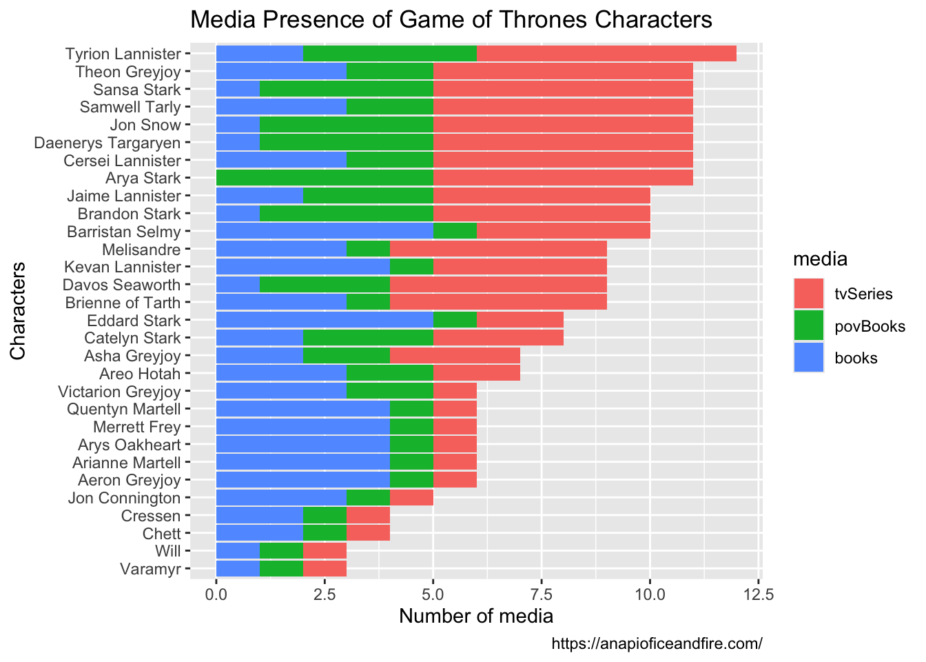
When I first ran this example from {repurrrsive}, I used books and tvSeries and not povbooks. When I plotted the data, I noticed Arya Stark has NA for books which, as a main character, seemed strange.
Use the open API at https://anapioficeandfire.com/ to get the data for Arya Stark to see if that is what the source data shows.
The following is a quick check from the original API source for the data which confirms Books is NA but povbooks has five of them.
Show code
# A tibble: 1 × 16
  url       name  gender culture born  died  titles aliases father mother spouse
  <chr>     <chr> <chr>  <chr>   <chr> <chr> <list> <list>  <chr>  <chr>  <chr>
1 https://… Arya… Female Northm… In 2… ""    <list> <list>  ""     ""     ""
# ℹ 5 more variables: allegiances <list>, books <lgl>, povBooks <list>,
#   tvSeries <list>, playedBy <list>
Perhaps, you want to know which characters have the most honorific title(s).
# A tibble: 6 × 2
  name                   n
  <chr>              <int>
1 Cersei Lannister       5
2 Daenerys Targaryen     5
3 Eddard Stark           5
4 Davos Seaworth         4
5 Kevan Lannister        4
6 Asha Greyjoy           3
The {tidyr} vignette has more examples of tidying even more complicated outputs from APIs.
6.12 Example: Rectangling NASA Data
6.12.1 The Data
The National Aeronautics and Space Administration’s SBDB Close-Approach Data (CAD) API provides access to current close-approach data (CAD) for all asteroids and comets in the California Institute of Technology’s Jet Propulsion Laboratory’s Small-Body DataBase.
Each CAD record is packaged as an array of fields (corresponding to those listed) in the following order:
- des: primary designation of the asteroid or comet (e.g., 443, 2000 SG344)
- orbit_id: orbit ID
- jd: time of close-approach (JD Ephemeris Time)
- cd: time of close-approach (formatted calendar date/time)
- dist: nominal approach distance (au)
- dist_min: minimum (3-sigma) approach distance (au)
- dist_max: maximum (3-sigma) approach distance (au)
- v_rel: velocity relative to the approach body at close approach (km/s)
- v_inf: velocity relative to a massless body (km/s)
- t_sigma_f: 3-sigma uncertainty in the time of close-approach (formatted in days, hours, and minutes;
- days are not included if zero; example “13:02” is 13 hours 2 minutes;
- example “2_09:08” is 2 days 9 hours 8 minutes)
- body: name of the close-approach body (e.g., Earth),
- only output if the body query parameters is set to ALL
- h: absolute magnitude H (mag)
- fullname: formatted full-name/designation of the asteroid or comet
- optional: only output if requested with the appropriate query flag.
- formatted with leading spaces for column alignment in mono-spaced font tables
- optional: only output if requested with the appropriate query flag.
6.12.2 Get the Most Recent Data and Save as RDS
Retrieve data for four lunar distances: 10, 20, 50, and 100.
- Here we create a request with all of the query elements but
dist-max. - We then add that value to the query before we run
req_perform(). - Note the need to use ` for the non-standard parameter names with a
-in them.
Save each response as an RDS file to enable analysis until the next update of data is needed.
- Make sure you have created an
06_datafolder.
request("https://ssd-api.jpl.nasa.gov/cad.api/") |>
  req_url_query(`date-min` = "2013-01-01") |>
  req_url_query(sort = "dist") |>
  req_url_query(body = "ALL") ->
req_nasa

req_nasa |>
  req_url_query(`dist-max` = "10LD") |>
  req_perform()  |>
  write_rds("./06_data/neo_data_10lu_2013.rds")

req_nasa |>
  req_url_query(`dist-max` = "20LD") |>
  req_perform()  |>
  write_rds("./06_data/neo_data_20lu_2013.rds")

req_nasa |>
  req_url_query(`dist-max` = "50LD") |>
  req_perform()  |>
  write_rds("./06_data/neo_data_50lu_2013.rds")

req_nasa |>
  req_url_query(`dist-max` = "100LD") |>
  req_perform()  |>
  write_rds("./06_data/neo_data_100lu_2013.rds")
6.12.3 Develop the Steps to Tidy and Clean the Data from one of the RDS files
Load the Near Earth Object (NEO) data from NASA close-approach data for NEOs within 10 lunar distances on or after 2013-Jan-01
- The
$bodyelement of the response has the information we want in RAW format.
[1] "httr2_response"List of 7
$ method : chr "GET"
$ url : chr "https://ssd-api.jpl.nasa.gov/cad.api/?date-min=2013-01-01&sort=dist&body=ALL&dist-max=10LD"
$ status_code: int 200
$ headers : <httr2_headers>
..$ date : chr "Sat, 11 May 2024 20:11:39 GMT"
..$ content-type: chr "application/json"
..$ server : chr "nginx"
..$ set-cookie : chr "AWSALBAPP-0=_remove_; Expires=Sat, 18 May 2024 20:11:39 GMT; Path=/"
..$ set-cookie : chr "AWSALBAPP-1=_remove_; Expires=Sat, 18 May 2024 20:11:39 GMT; Path=/"
..$ set-cookie : chr "AWSALBAPP-2=_remove_; Expires=Sat, 18 May 2024 20:11:39 GMT; Path=/"
..$ set-cookie : chr "AWSALBAPP-3=_remove_; Expires=Sat, 18 May 2024 20:11:39 GMT; Path=/"
$ body : raw [1:2085973] 7b 22 73 69 ...
$ request :List of 7
..$ url : chr "https://ssd-api.jpl.nasa.gov/cad.api/?date-min=2013-01-01&sort=dist&body=ALL&dist-max=10LD"
..$ method : NULL
..$ headers : list()
..$ body : NULL
..$ fields : list()
..$ options : list()
..$ policies: list()
..- attr(*, "class")= chr "httr2_request"
$ cache :<environment: 0x843a8f268>
- attr(*, "class")= chr "httr2_response"Convert to a list of JSON.
The data we want is the vector of variable names in $fields and the list in $data.
We need to combine the elements from $fields and $data to create the tibble we want.
- Convert
datato a tibble usingtibble(). - Unnest the list column to create more columns and save as a new tibble.
- Set the new tibble column names equal to the values from
$fields(after unlisting to create a vector).
Rows: 11,317
Columns: 12
$ des       <chr> "2024 JV8", "2020 VT4", "2020 QG", "2021 UA1", "2023 BU", "2…
$ orbit_id  <chr> "2", "5", "4", "3", "22", "1", "27", "2", "2", "27", "3", "5…
$ jd        <chr> "2460362.065008999", "2459167.222686305", "2459077.672759561…
$ cd        <chr> "2024-Feb-21 13:34", "2020-Nov-13 17:21", "2020-Aug-16 04:09…
$ dist      <chr> "1.95292215627956e-05", "4.50910597356063e-05", "6.227979849…
$ dist_min  <chr> "0", "4.50230750909071e-05", "6.22040307793404e-05", "6.2949…
$ dist_max  <chr> "0.000112897191731237", "4.51593933094878e-05", "6.235555619…
$ v_rel     <chr> "2.01472928494528", "13.4271195491719", "12.3308673063873", …
$ v_inf     <chr> "0.838337877552835", "7.88069685599943", "8.15386324007669",…
$ t_sigma_f <chr> "10:14", "< 00:01", "< 00:01", "< 00:01", "< 00:01", "< 00:0…
$ body      <chr> "Moon", "Earth", "Earth", "Earth", "Earth", "Earth", "Moon",…
$ h         <chr> "26.242", "28.61", "29.90", "31.84", "29.70", "32.32", "31.7…
Everything is still character so we can clean the variable types and create a new variable for the minimum distance in Lunar Distances based on the dist_min which is in astronomical units.
- Note: 1 Lunar Distance = 384,317 Kilometers = 0.002569 astronomical units (au).
Rows: 11,317
Columns: 13
$ des         <chr> "2024 JV8", "2020 VT4", "2020 QG", "2021 UA1", "2023 BU", …
$ orbit_id    <dbl> 2, 5, 4, 3, 22, 1, 27, 2, 2, 27, 3, 5, 3, 1, 4, 3, 3, 4, 1…
$ jd          <dbl> 2460362, 2459167, 2459078, 2459513, 2459972, 2460195, 2458…
$ cd          <dttm> 2024-02-21 13:34:00, 2020-11-13 17:21:00, 2020-08-16 04:0…
$ dist        <dbl> 1.952922e-05, 4.509106e-05, 6.227980e-05, 6.301350e-05, 6.…
$ dist_min    <dbl> 0.000000e+00, 4.502308e-05, 6.220403e-05, 6.294948e-05, 6.…
$ dist_min_ld <dbl> 0.00000000, 0.01752553, 0.02421332, 0.02450350, 0.02593414…
$ dist_max    <dbl> 1.128972e-04, 4.515939e-05, 6.235556e-05, 6.307751e-05, 6.…
$ v_rel       <dbl> 2.014729, 13.427120, 12.330867, 15.835007, 9.267245, 13.58…
$ v_inf       <dbl> 0.8383379, 7.8806969, 8.1538632, 12.8910404, 2.4284938, 10…
$ t_sigma_f   <dbl> 10, 0, 0, 0, 0, 0, 0, 0, 0, 0, 0, 0, 0, 0, 0, 0, 0, 0, 0, …
$ body        <fct> Moon, Earth, Earth, Earth, Earth, Earth, Moon, Earth, Moon…
$ h           <dbl> 26.242, 28.610, 29.900, 31.840, 29.700, 32.320, 31.740, 32…
6.12.4 Create Functions to Tidy and Clean
We have multiple .RDS files so instead of copy and paste, let’s build some helper functions.
- We want to load, tidy, and clean the data for any .rds file saved from this API.
- It should work on objects of class “httr2_response.”
Strategy:
- Generate/load the response data
- Extract the content from the response using
resp_body_json()which will be returned as list. - Convert the list to a tibble using
tibble(). - Unnest the list column into to multiple columns with minimal names.
- Set the tibble column names equal to the values from the
$fieldselement. - Use a second helper function to clean the data.
Create a vector with the paths to the .rds files.
Write the “clean” function since we will want to source it and use it in the “tidy” function.
Write the “tidy” function and call the “clean” function at the end.
- I added a step to add a column to each data frame that has the Lunar Distance as identified from the data frame. It pulls from the URL used in the query for the original API call.
- Note: the first several steps are general to many APIs.
- By changing out the “clean” function and later steps you could customize the cleaning to other APIs.
tidy_nasa_neo <- function(response) {
stopifnot(class(response) == "httr2_response")
resp_body_json(response) ->
temp_list
tibble(value = temp_list$data) |> # the _ pronoun from the natural pipe
unnest_wider(value, names_sep = "") ->
temp_df
names(temp_df) <- unlist(temp_list$fields)
## what follows customized to neo-cad data
temp_df <- clean_neo_df(temp_df)
temp_df <- mutate(temp_df,
ld = as.numeric(response$url |> str_extract("(?<=max=).+(?=LD)")),
.before = everything()
)
temp_df
}Now we can use map() to run the function for our list of files which will create a list.
Since each data frame will be the same we can put all the data into one large tibble using list_rbind().
# A tibble: 6 × 14
ld des orbit_id jd cd dist dist_min dist_max
<dbl> <chr> <dbl> <dbl> <dttm> <dbl> <dbl> <dbl>
1 10 2024 JV8 2 2460362. 2024-02-21 13:34:00 1.95e-5 0 1.13e-4
2 10 2020 VT4 5 2459167. 2020-11-13 17:21:00 4.51e-5 4.50e-5 4.52e-5
3 10 2020 QG 4 2459078. 2020-08-16 04:09:00 6.23e-5 6.22e-5 6.24e-5
4 10 2021 UA1 3 2459513. 2021-10-25 03:07:00 6.30e-5 6.29e-5 6.31e-5
5 10 2023 BU 22 2459972. 2023-01-27 00:29:00 6.66e-5 6.66e-5 6.66e-5
6 10 2023 RS 1 2460195. 2023-09-07 14:26:00 6.93e-5 6.92e-5 6.94e-5
# ℹ 6 more variables: v_rel <dbl>, v_inf <dbl>, t_sigma_f <dbl>, body <fct>,
# h <dbl>, dist_min_ld <dbl>6.12.5 Create Helper Functions to Plot and Explore the Data
6.12.5.1 Does the Number of Objects Vary with Minimum Approach Distance and Body
Plot the distribution of the minimum distance of objects by body
Create two helper functions
- The first is for adjusting the position of the labels on the plot
- The second is to create the plots.
give.n <- function(x) {
c(y = median(x) * 1.4, label = length(x))
## experiment with the multiplier to find a good position
}
plot_df <- function(df) {
ggplot(df, aes(x = body, y = dist_min_ld)) +
geom_boxplot() +
ggtitle(paste0(
df$ld,
" LD: ",
format(nrow(df), big.mark = ","), " Objects"
)) +
xlab("") +
ylab("Min App Dist") +
coord_flip() +
stat_summary(
fun.data = give.n, geom = "text", fun = median,
position = position_dodge(width = 0.75)
) ->
my_return_value
return(my_return_value)
}Use map() with the plot helper function to create a list where the elements are a plot for each tibble in the list.
- You can use Quarto layout parameters to plot multiple plots at once Figures.
- You can also use the {patchwork} package to plot all at once with nmore flexibility.
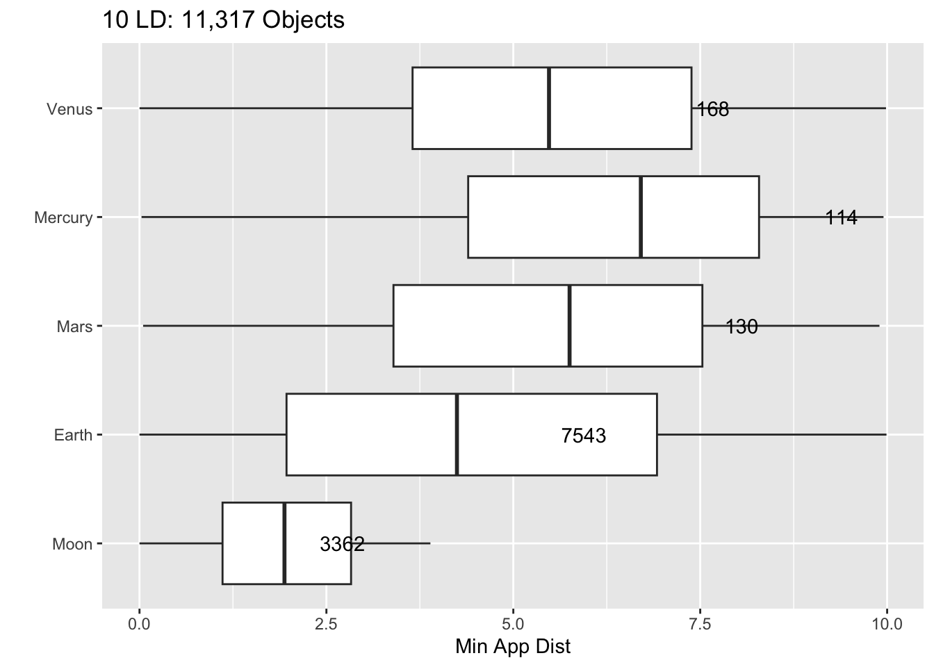
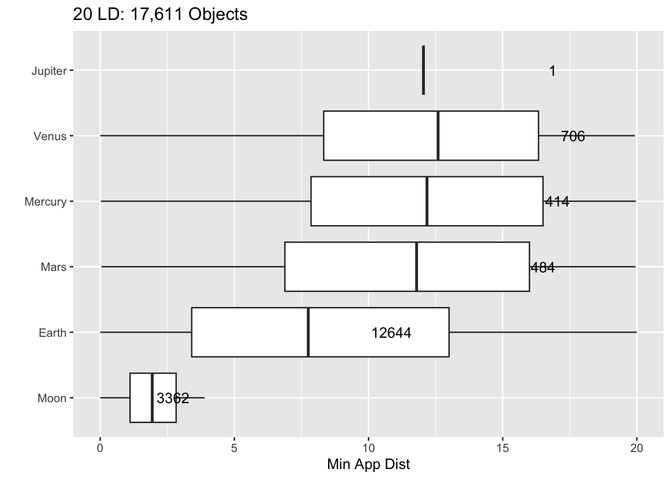
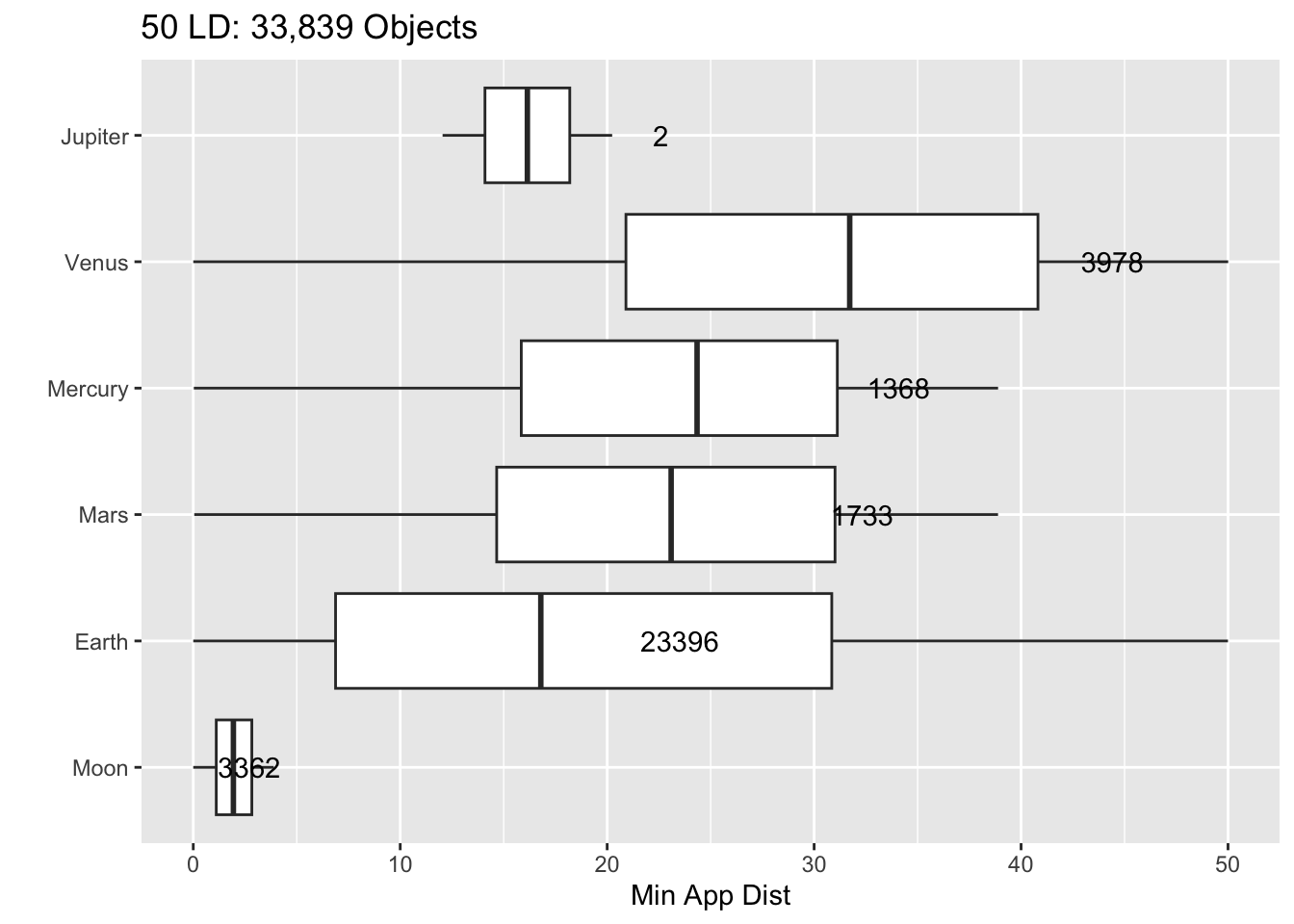
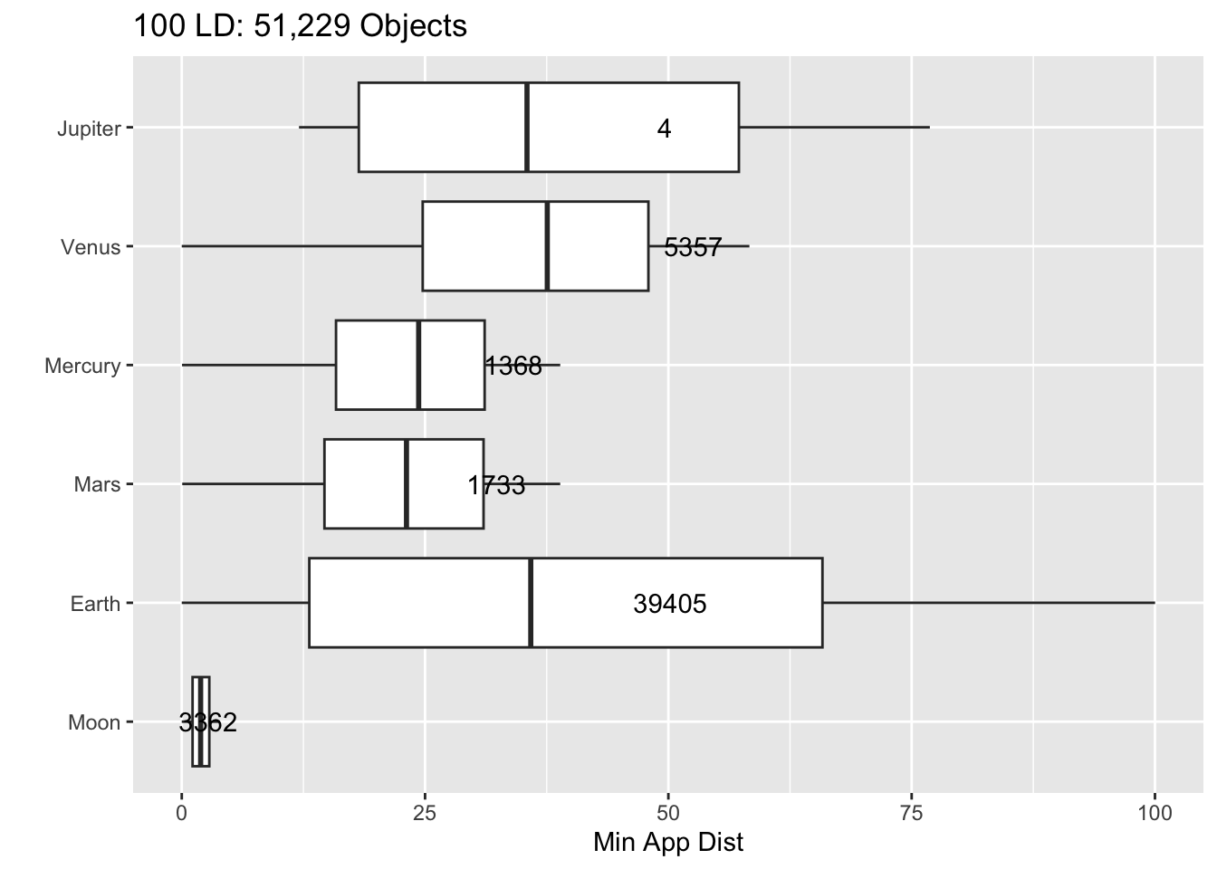
There appears to be a difference between the Earth and the moon that does not make physical/geometric sense. We’ll explore in a few steps.
6.12.5.2 Does the Number of Objects vary by Day of the Week?
Plot the total number of objects by day of the week by body
Let’s create a second plot function for day of the week.
plot_dow <- function(df) {
df |>
mutate(wkday = lubridate::wday(cd)) |>
group_by(wkday, body) |>
summarize(tot_des = n(), .groups = "drop") |>
ggplot(aes(x = wkday, y = tot_des, color = body)) +
geom_line() +
scale_y_log10() +
ggtitle(paste0(
df$ld,
" LDs: ",
format(nrow(df), big.mark = ","), " Objects"
)) +
xlab("Weekday") +
ylab("Num Objects") +
theme(legend.position = "top") +
scale_color_discrete(name = " ")
}Now plot.
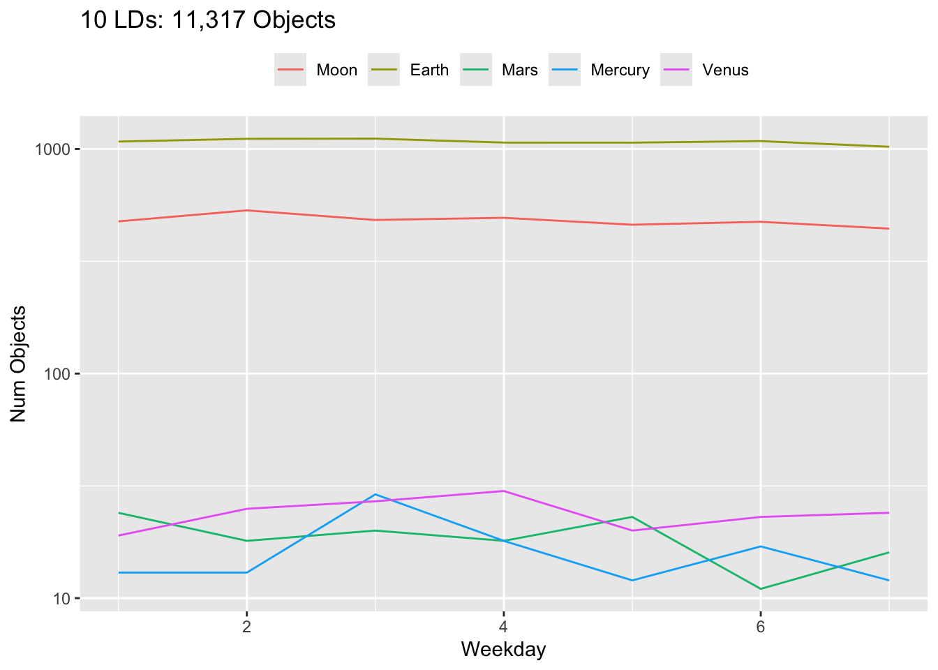
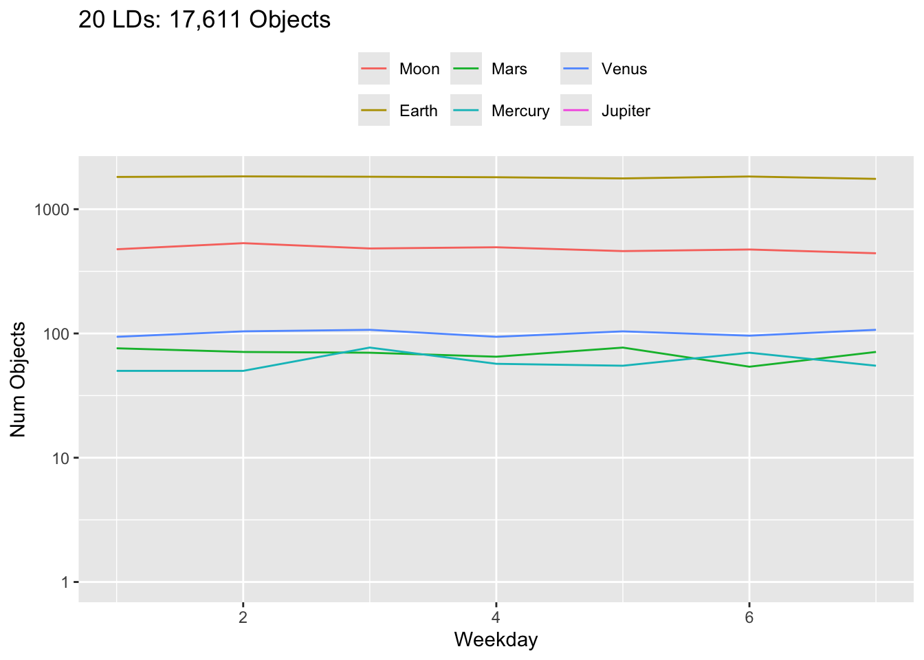
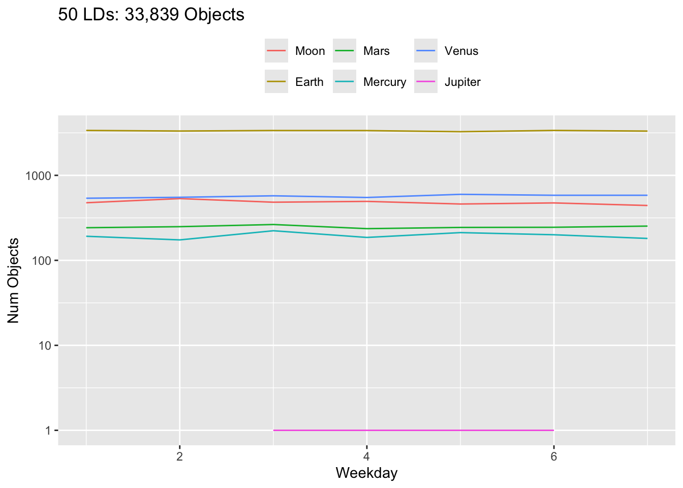
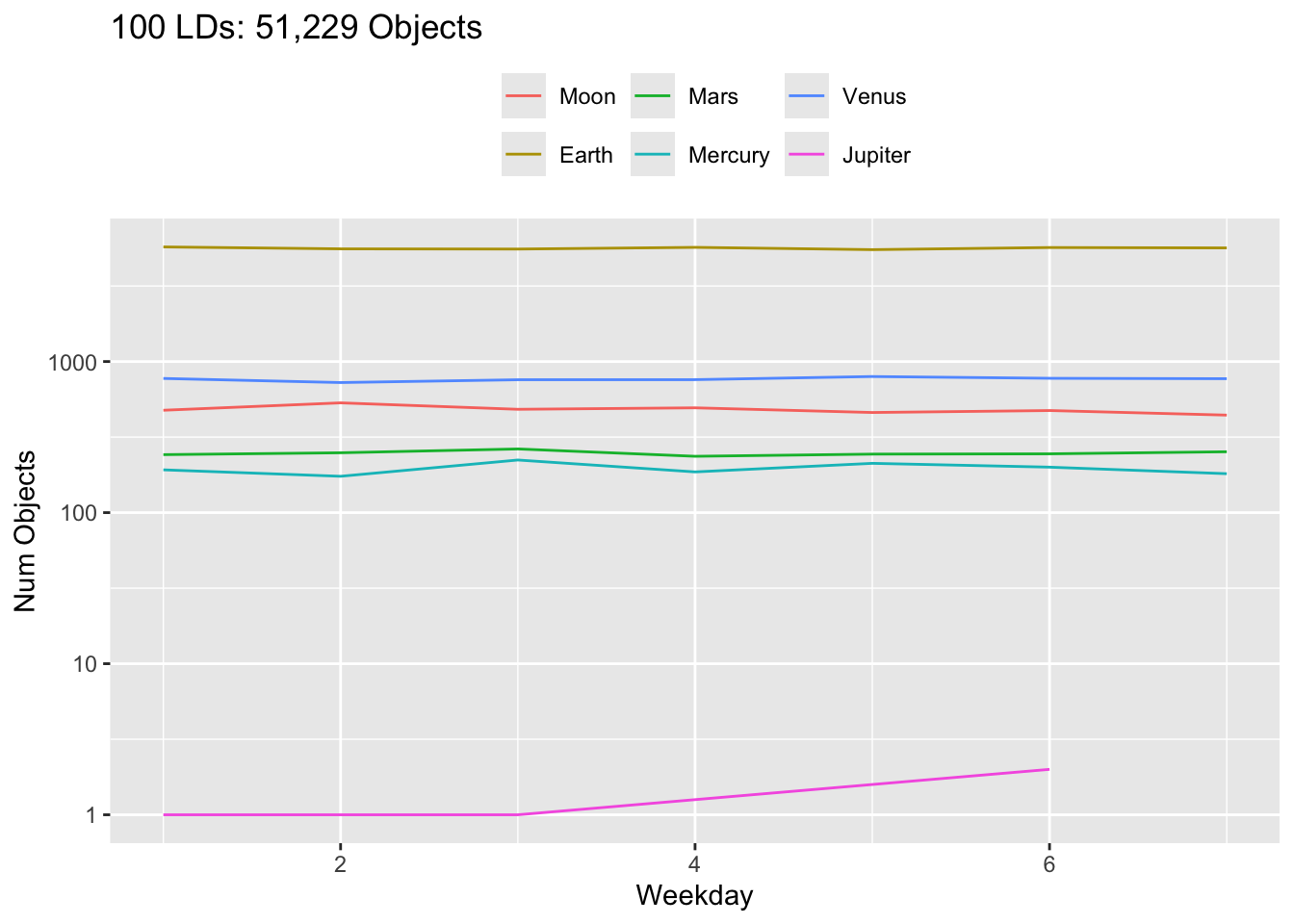
- There appear to be some anomalies across the days of the week.
- Run an analysis of variance for 10 and 50 LDs to see what might be happening?
Df Sum Sq Mean Sq F value Pr(>F)
body 4 6091874 1522968 6209.210 < 2e-16 ***
wkday 1 2169 2169 8.841 0.00644 **
body:wkday 4 2498 624 2.546 0.06448 .
Residuals 25 6132 245
---
Signif. codes: 0 '***' 0.001 '**' 0.01 '*' 0.05 '.' 0.1 ' ' 1 Df Sum Sq Mean Sq F value Pr(>F)
body 5 51819815 10363963 15831.373 <2e-16 ***
wkday 1 232 232 0.354 0.557
body:wkday 5 4678 936 1.429 0.248
Residuals 25 16366 655
---
Signif. codes: 0 '***' 0.001 '**' 0.01 '*' 0.05 '.' 0.1 ' ' 1There appears to be some evidence for a difference in the days when looking at only 10 LDs for some bodies. However, those bodies have relatively small sample sizes so require more analysis of the assumptions to see if the difference is real.
6.12.5.3 Assess the Differences Between the Earth and the Moon
Plot Objects going by both Moon and Earth.
Create another plot function.
plot_m_e_o <- function(df) {
df |>
filter(body %in% c("Earth", "Moon")) |> ## Only objects for Moon and Earth
group_by(des) |> ## for each object
mutate(n_bodies = length(unique(body)), .after = body) |> ## how many bodies
ungroup() |>
filter(n_bodies > 1) |> ## Select objects that pass both Earth and Moon
group_by(des, body) |> ## for each object and body
filter(dist_min_ld == min(dist_min_ld)) -> tt ## Select the pass with the minimum distance
ggplot(tt, aes(x = body, y = dist_min_ld)) +
geom_boxplot() +
stat_summary(
fun.data = give.n, geom = "text", fun = median,
position = position_dodge(width = 0.75)
) +
ggtitle(paste0(
df$ld,
" LDs: ",
format(nrow(df), big.mark = ","), " Objects"
)) +
xlab("Weekday") +
ylab("Num Objects") +
theme(legend.position = "top") +
scale_color_discrete(name = " ")
}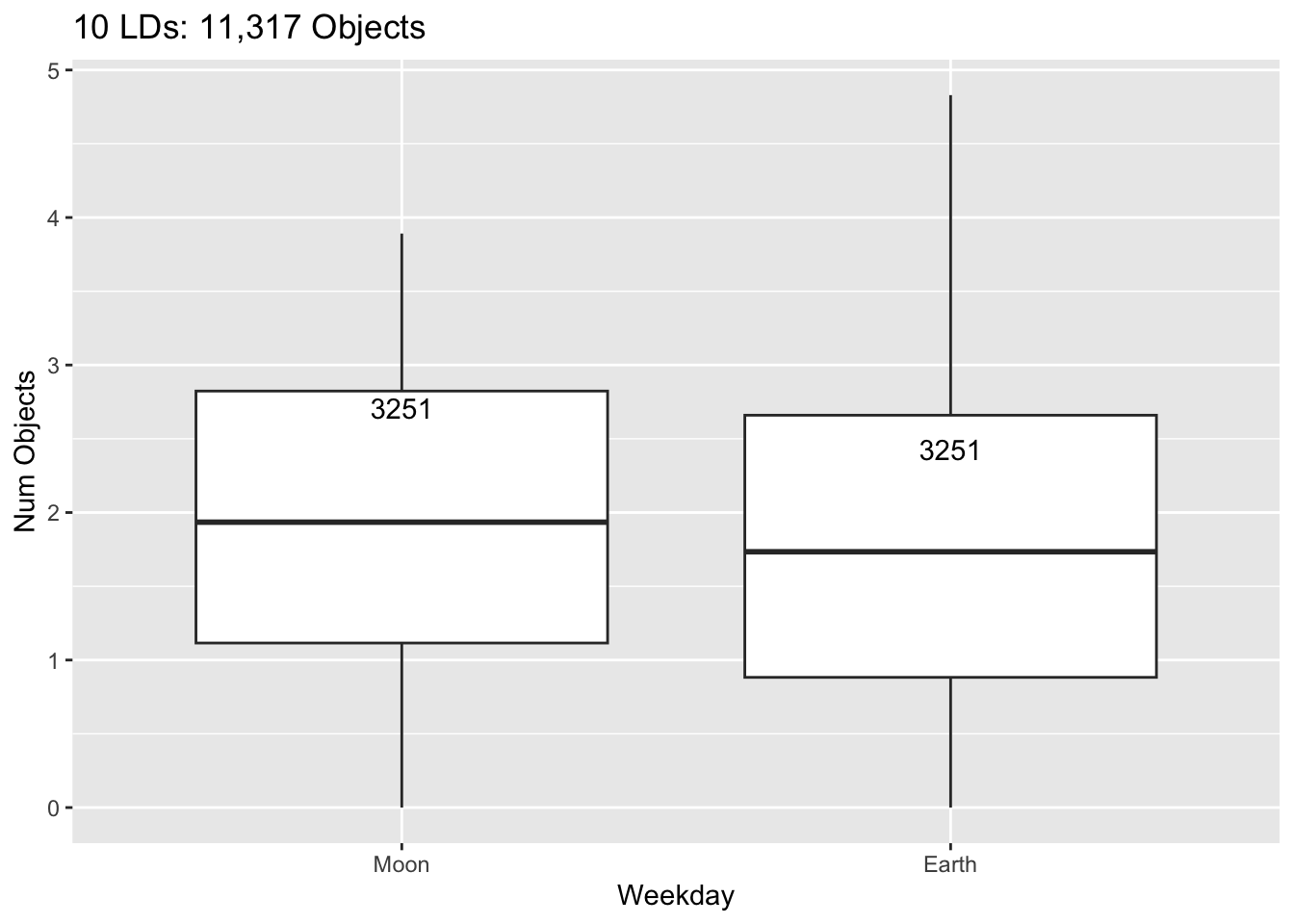
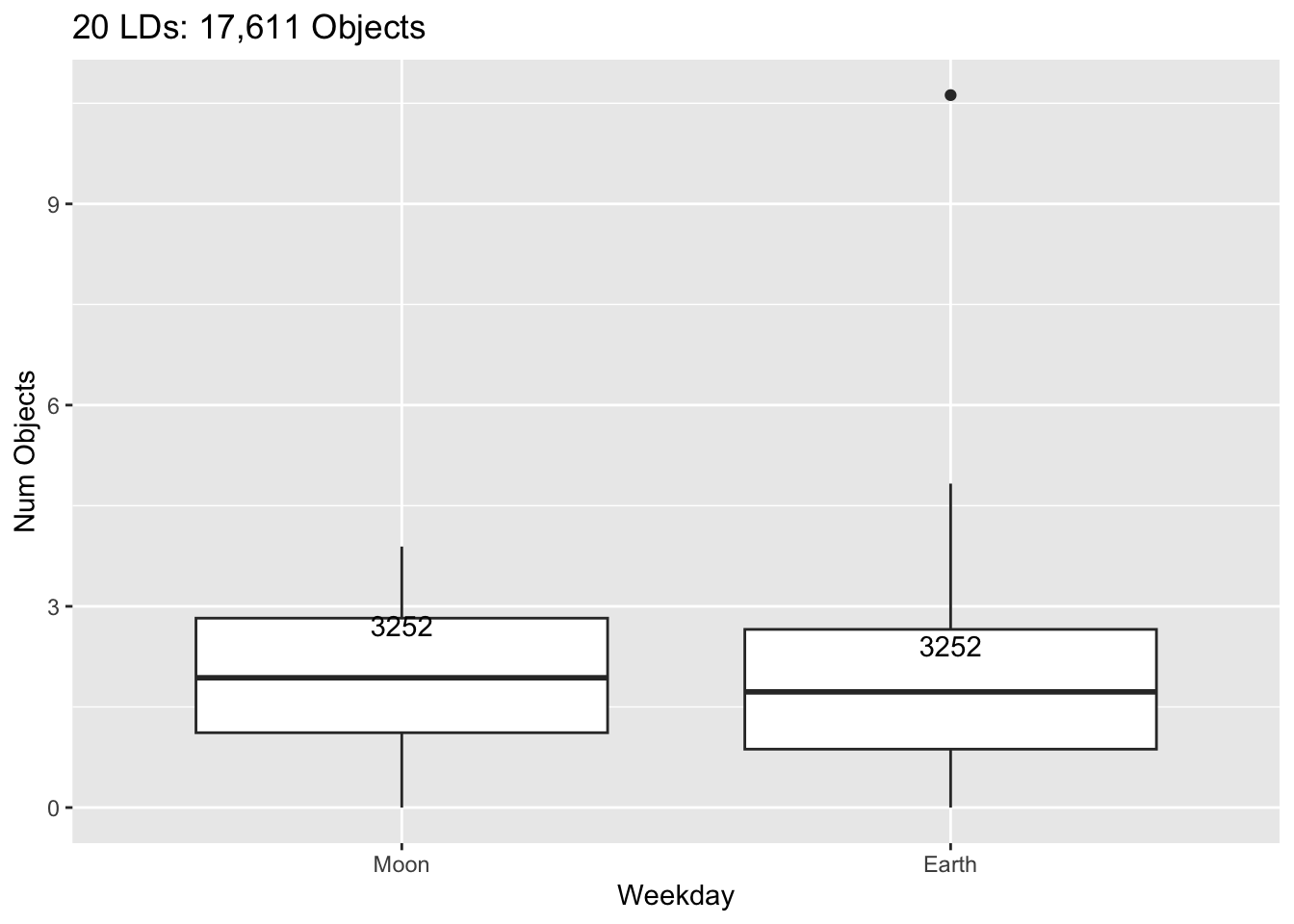

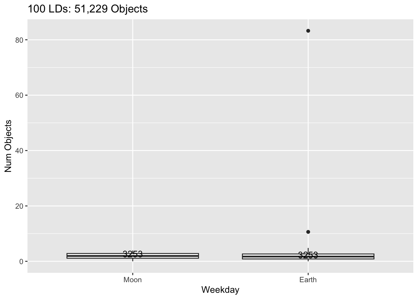
Plot Objects going only by Earth or Moon (1)
plot_m_or_e <- function(df) {
df |>
filter(body %in% c("Earth", "Moon")) |> ## Only objects for Moon and Earth
group_by(des) |> ## for each object
mutate(n_bodies = length(unique(body)), .after = body) |> ## how many bodies
ungroup() |>
## filter(n_bodies > 1) |> #Select objects that pass both Earth and Moon
group_by(des, body) |> ## for each object and body
filter(dist_min_ld == min(dist_min_ld)) -> tt ## Select the pass with the minimum distance
ggplot(tt, aes(x = body, y = dist_min_ld)) +
geom_boxplot() +
facet_grid(~n_bodies) +
stat_summary(
fun.data = give.n, geom = "text", fun = median,
position = position_dodge(width = 0.75)
) +
ggtitle(paste0(
df$ld,
" LDs: ", nrow(tt), " Objects \n(1 = E or M and 2 = Both E and M)"
))
}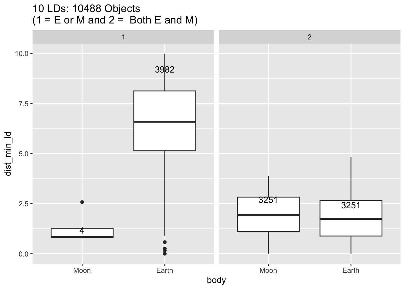
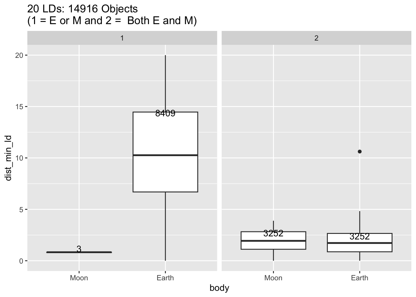
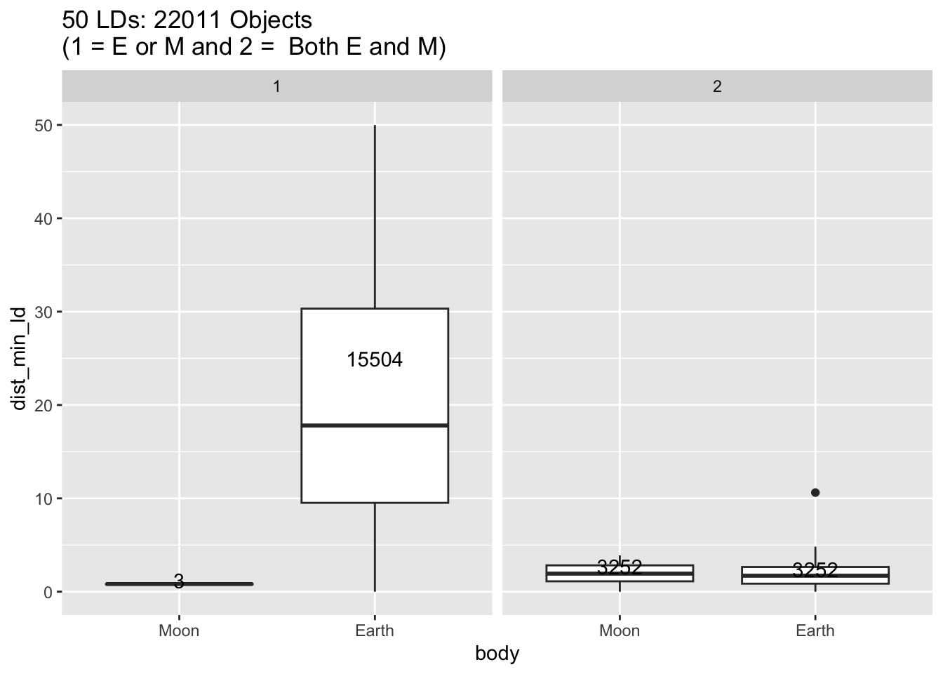

6.12.5.4 What is Happening?
After asking the SBDB team, it turns out there are hard limits imposed on the API on each close-approach body to keep the returned data set of reasonable size and still ensure detection of close-approaches of interest.
- For example, the limit for Venus is 0.15 au, for Earth is 0.5 au, and for the moon is 0.01 au (about 4 LD).
- That is why the Earth has far more objects than the moon.
Tip
Don’t be afraid to reach out to a data-source owner or the community to ask questions when the data does not seem to make sense!
6.12.6 Summary for Rectangling
Data returned from APIs can be in different structures and often in deeply-nested lists when converted from JSON.
The {tidyr} package provides many functions to facilitate manipulating deeply nested lists so you can access the data you want for your analysis while keeping all of the data for future work.