11 Shiny Layouts Plus
R Shiny, reactivity, shiny layouts, HTML, widgets, CSS, shinyapps.io, shiny modules
11.1 Introduction
11.1.1 Learning Outcomes
- Use Shiny “reactive” elements for efficient design and control of a Shiny app.
- Create Shiny apps with different user interface layouts.
- Customize the look and feel of a Shiny app.
- Incorporate HTML widgets into a Shiny app.
- Upload data into a Shiny app.
- Deploy a working Shiny app.
- Incorporate functions to streamline your Shiny apps.
11.1.2 References:
- Mastering Shiny Wickham (2022)
- Application Layout Guide Allaire (2021)
- {fresh} R package Perrier (2023)
- Customize your UI with HTML Grolemund et al. (2017)
- Bootswatch Themes Park (2023)
- {thematic} package Sievert et al. (2022)
- HTML Widgets for R Vaidyanathan and Russell (2015)
- {plotly} package Sievert (2020)
- {rpivotTable} package Martoglio (2018)
- {tmap} package Tennekes (2023)
- Share Your Shiny Applications Online Posit (2023)
- shinyapps.io user guide team (n.d.)
- Modularizing Shiny app code Chang (2020)
- Engineering Production-Grade Shiny Apps Fay et al. (2023)
11.1.2.1 Other References
- R for Data Science 2nd Edition Wickham et al. (2023)
- Shiny Cheatsheet.
bindEvent()articlebindCache()article- Outstanding User Interfaces with Shiny Granjon (2022)
- bslib Package Sievert et al. (2023)
- CSS Schools (2023)
- {bslib} bootstrap 5 library Radečić (2022)
- Shiny HTML Tags Glossary Grolemund (2017)
- {plotly} GitHub Sievert (2023)
- tmap: Elegant and Informative Maps with tmap Tennekes and Nowosad (2021)
- {vroom} package Hester et al. (2023)
- Getting Started with shinyapps.io
- {rsconnect} Package Atkins et al. (2023)
- Eric Nantz Talk at RStudioConf 2019 Nantz (2019)
Shiny provides many, many, many different options for designing and customizing a Shiny app.
To avoid getting overwhelmed, it helps to follow the design strategy for a minimum viable product as seen in Figure 11.1 from Fay et al. (2023).
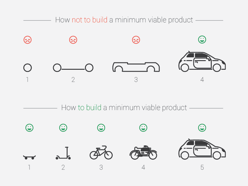
Don’t try to build everything at once!
- People users want to see working products that progress, not promises things will work.
Have an idea of what you want it to look like at the end and create a high-level design.
Follow the mantra of build-a-little-test-a-little.
- Use Git branches to protect the working Main branch.
- Use the debugging tools for the business logic and server code.
- The smaller pieces you build before testing, the easier to debug any errors.
The elements are the cake and the customization is the icing.
- Make sure it works before you spend time on customization.
Don’t be afraid to experiment. When you see an opportunity to move code out of the server into the business logic as a custom function, do it.
Commit and push your branch often.
Get feedback from others early and often to update your design.
11.2 Introduction to Reactivity in Shiny
In Shiny, you express your server logic using reactive programming.
- Reactive programming is elegant and powerful but it can be disorienting as the flow is different than what occurs in an R script.
The key idea of reactive programming is for the code to create, behind the scenes, a network “graph” of dependencies so, when an input changes, all dependent (related) outputs are automatically updated.
- It would be easy to run all the code to update everything any time one input changes, but that would be inefficient and slow for the user.
- The reactive graph of dependencies ensures only the downstream dependencies are updated (while ignoring elements that don’t need to be updated).
- Reactivity makes the flow of an app considerably simpler, but it can take a while to get your head around how it all fits together.
Reactivity enables shiny’s declarative programming structure:
- The code declares (tells) how to create output and then sets the conditions for when code is to be executed (the reactivity recipes) but does not say in what sequence the code should or will be executed.
- The Shiny back end manages code execution when the app is running (and reacting to user inputs).
Thus the code in Shiny Apps does Not flow top-to-bottom like a standard (imperative) R script.
- Debugging shiny code can be challenging as the shiny model is different than we are used to.
- You can use the debugging tools on code in the business logic and server sections.
A design goal is to minimize the amount of reactive code to make it easier to debug and maintain.
When practical, create or source custom functions in the (non-reactive) business section and then you can call them in the (reactive) server sections.
This allows you to debug the custom functions in the usual way while reducing the amount of code in the server section.
11.2.1 The Server Function
- Recall, the server function always looks like this:
11.2.1.1 The input Argument
A list-like object created by the input() function.
- It has the IDs for all the elements in the UI that the
server()function can access.- Each element should have been created by an input function in the UI.
- Each element can only be accessed by
server()through a reactive function.- This will be either a
render*()function or in areactive()call. - Example, the following will throw an error:
- This will be either a
11.2.1.2 The output: Argument
A list-like object created by the ui() function with the names of the UI’s output elements.
- You write code in the
server()function which modifies the individual elements ofoutput$namewhich are then used by updated for presentation by theui() function. - You use one of the many different types of
render*()functions to modify elements ofoutput.- You’ll get an error if you don’t use a
render*()function.
- You’ll get an error if you don’t use a
11.2.2 Render Functions
- You’ve already seen render functions. They are of the form below, where the
*is replaced by the type of output object to be rendered:
The output of a render*() function is assigned to an element of the output list.
- The
render*()function type (the*) must match the type established for the named element in the UI code- Example: the UI element
textOutput("text")gets assigned output in the server code fromrenderText(). - Functions include:
renderText(),renderPrint(),renderPlot(),renderCachedPlot(),renderTable(),renderDataTable(), andrenderImage().
- Example: the UI element
- The curly braces inside the
render*()function mean you can write an expression which then becomes the “argument” of therender*()function.- An expression can be one or many lines of code (just like when writing a function).
Since shiny is reactive, if any input elements inside the render*() function get changed, they will trigger the render*() code to be re-evaluated, updating the output elements.
- When an input element changes, it is said to be “invalidated”. This triggers the reactive elements.
- When any input in a inside a reactive code chunk is invalidated, Shiny will rerun the entire code chunk (not just the portion that was invalidated).
Create a Shiny App that asks for a person’s name and then prints “Hello” followed by the person’s name.
11.2.3 Reactive Expressions
You can create variables via the reactive expression reactive({}).
- These are more precisely referred to as “reactive elements” or “reactive values”.
They can then be reused in different reactive expressions or render*() functions.
library(shiny)
library(stringr)

ui <- fluidPage(
  textInput("text", "What Text?", value = "dog"),
  textOutput("pigtext1"),
  textOutput("pigtext2")
)

server <- function(input, output) {
  x <- reactive({
    str_replace(input$text, "([^aeiouAEIOU]*)(.*)", "\\2\\1ay")
    # find the first set of non-vowels as group1 and
    # the rest of the input as group2
    # put group2 first then the group 1 consonants followed by "ay"
  })
  output$pigtext1 <- renderText(c("Original: ", input$text))
  output$pigtext2 <- renderText(c("PL Translation: ", x()))
}

shinyApp(ui = ui, server = server)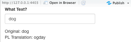
Let’s rewrite to use a custom function in the business logic section and reduce the code in the server section.
library(shiny)
library(stringr)
pigl <- function(textt) {
  str_replace(textt, "([^aeiouAEIOU]*)(.*)", "\\2\\1ay")
}

ui <- fluidPage(
  textInput("text", "What Text?", value = "dog"),
  textOutput("pigtext1"),
  textOutput("pigtext2")
)

server <- function(input, output) {
  x <- reactive({
    pigl(input$text)
    # find the first set of non-vowels as group1 and
    # the rest of the input as group2
    # put group2 first then the group 1 consonants followed by "ay"
  })
  output$pigtext1 <- renderText(c("Original: ", input$text))
  output$pigtext2 <- renderText(c("PL Translation: ", x()))
}

shinyApp(ui = ui, server = server)- The
pigl()function is Not reactive and could be debugged in a normal R script.
You can use reactive in render*() functions, but include a () after them (like function calls, as technically, they are functions.
- We can define a reactive element
xto depend uponinput$textusingreactive()as follows.
But when we call it later, we need to “call” it with ().
The name x is bound to the expression and not a single value so we have to call it to have the expression evaluated with the current values of its inputs.
- If you didn’t use
reactive(), you would get an error because you would be callinginput$textoutside of arender*()orreactive()call.
An example with simulation data.
library(shiny)
library(tidyverse)
library(broom)

ui <- fluidPage(
  numericInput("nsamp", "Number of samples", value = 50, step = 1),
  numericInput("diff", "Effect size", value = 0.5, step = 0.1),
  plotOutput("plot"),
  tableOutput("text")
)

server <- function(input, output) {
  x1 <- reactive({
    rnorm(n = input$nsamp, mean = 0, sd = 1)
  })

  x2 <- reactive({
    rnorm(n = input$nsamp, mean = input$diff, sd = 1)
  })

  output$plot <- renderPlot({
    data.frame(`1` = x1(), `2` = x2())  |>
      pivot_longer(
        cols = everything(),
        names_to = "Group",
        values_to = "y"
      ) |>
      ggplot(aes(x = Group, y = y)) +
      geom_boxplot() +
      theme_bw()
  })

  output$text <- renderTable({
    t.test(x1(), x2())  |>
      tidy() |> # use of tidy() converts from Code output to table output
      select(estimate,
        `P-value` = p.value,
        Lower = conf.low,
        Higher = conf.high
      )
  })
}

shinyApp(ui = ui, server = server)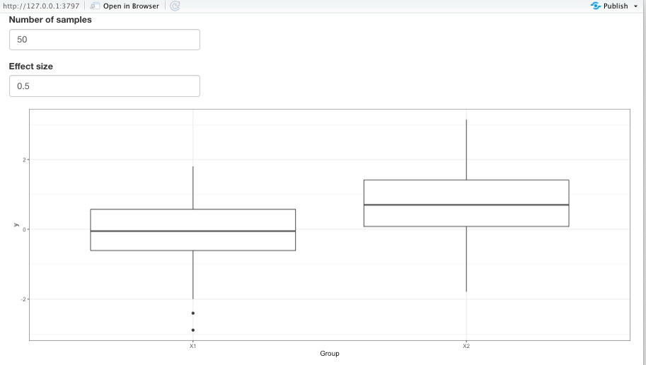
Create a Shiny App with a slider that accepts input for sample size and then simulates a sample of that size from a standard normal distribution and outputs a histogram of the data and the output of summary().
Show code
library(shiny)
library(ggplot2)

ui <- fluidPage(
  sliderInput("nsamp", "Sample Size", value = 50, min = 1, max = 200),
  plotOutput("plot"),
  verbatimTextOutput("summary")
)

server <- function(input, output, session) {
  samp <- reactive({
    rnorm(input$nsamp)
  })

  output$plot <- renderPlot({
    qplot(samp(), bins = 20)
  })

  output$summary <- renderPrint({
    summary(samp())
  })
}

shinyApp(ui, server)
11.2.4 More on Reactive Programming
Shiny only runs the reactive code in the server function when the inputs have changed.
As mentioned earlier, in usual R, the order of operations is defined by the order or sequence of the lines of code (ignoring for-loops and if statements). This is a form of “imperative” programming.
In Shiny, the order of operations is defined by the order of when things are needed to run. This is a form of “declarative” programming.
- When an input changes, Shiny calls this “invalidation” and it causes the
render*()functions and reactive elements affected by the changed input to rerun.
11.2.4.1 Timed Invalidation using reactiveTimer()
You can cause invalidation in time intervals (so the reactive elements will reevaluate) using reactiveTimer().
- A crude form of animation perhaps
reactiveTimer() creates a reactive element that invalidates based on a time interval.
- The time interval argument is
intervalsMs =for how often to fire, in milliseconds
To re-simulate new data every second, put a reactiveTimer() element, with argument intervalMs = 1000, inside the code chunk with the reactive elements you wish to invalidate, and thus recalculate, in timed intervals.
library(shiny)
library(tidyverse)
library(broom)

# moving the t.test function to the business logic section
tt_output <- function(x, y) {
  t.test(x, y) |>
    broom::tidy() |>
    dplyr::select(estimate,
      `P-value` = p.value,
      Lower = conf.low,
      Higher = conf.high
    )
}

ui <- fluidPage(
  numericInput("nsamp", "Number of samples", value = 50, step = 1),
  numericInput("diff", "Effect size", value = 0.5, step = 0.1),
  plotOutput("plot"),
  tableOutput("text")
)

server <- function(input, output) {
  timer1 <- reactiveTimer(1000)

  x1 <- reactive({
    timer1() # note the use of ()
    rnorm(n = input$nsamp, mean = 0, sd = 1)
  })

  x2 <- reactive({
    timer1() # note the use of ()
    rnorm(n = input$nsamp, mean = input$diff, sd = 1)
  })

  output$plot <- renderPlot({
    data.frame(`1` = x1(), `2` = x2()) |>
      pivot_longer(cols = everything(), names_to = "Group", values_to = "y") |>
      ggplot(aes(x = Group, y = y)) +
      geom_boxplot() +
      theme_bw()
  })

  output$text <- renderTable({
    tt_output(x1(), x2())
  })
}

shinyApp(ui = ui, server = server)Create a Shiny App that uses a slider to accept input for sample size from 1 to 200 and then simulates a sample of that size from a standard normal distribution and outputs a histogram of the data and the output of summary().
- Make it automatically simulate new data once every two seconds.
Show code
library(shiny)
library(ggplot2)

ui <- fluidPage(
  sliderInput("nsamp", "Sample Size", value = 50, min = 1, max = 200),
  plotOutput("plot"),
  verbatimTextOutput("summary")
)

server <- function(input, output, session) {
  timer2 <- reactiveTimer(2000)

  samp <- reactive({
    timer2()
    rnorm(input$nsamp)
  })

  output$plot <- renderPlot({
    qplot(samp(), bins = 20)
  })

  output$summary <- renderPrint({
    summary(samp())
  })
}

shinyApp(ui, server)11.2.4.3 eventReactive()
The original solution was to use an actionButton() in the UI along with eventReactive() in the server function to do this.
eventReactive()was used in place ofreactive().- Takes the
actionButton()ID as its first argument. - Takes the expression to evaluate as its second argument.
- Takes the
- As of {shiny} 1.6.0 there is a new function called
bindEvent()which can replaceeventReactive()and is the recommended approach.
11.2.4.4 Observe User actions with observeEvent()
If you want to run code whose output does not need to be saved to an object, the older approach was to use observeEvent() instead of eventReactive().
- This could be saving data to a file, or printing to the console, or downloading a pre-specified file from the internet.
- Note: You cannot save the output of a call to
observeEvent().
- Note: You cannot save the output of a call to
- This has also been replaced by
bindEvent()as the recommended approach.
11.2.4.5 Using bindEvent() to Control When Invalidation Occurs for an Object
As of {shiny} 1.6.0, there is a new function called bindEvent() which allows you control when a reactive object (created as a result of reactive() or render*() function) “reacts” or becomes invalidated.
- Note this is newer than the new Mastering Shiny book so see the optional reference on
bindEvent()
Normally, reactive events become invalidated when any of the inputs change or become invalidated themselves.
bindEvent() allows you to set conditions for controlling when a reactive object becomes invalidated
- The first argument of
bindEvent()is the reactive object you want to modify, so, you can pipe into it from thereactive(). bindEvent()also offers more flexibility as it can be used withrender*()functions.- It can also be used with
bindCache()to speed up server operations. See Using caching in Shiny …
11.2.4.5.1 Example of bindEvent() to Replace eventReactive()
Note the piping of the reactive object into bindEvent() as the first argument.
library(shiny)
library(tidyverse)
library(broom)

tt_output <- function(x, y) {
  t.test(x, y) |>
    broom::tidy() |>
    dplyr::select(estimate,
      `P-value` = p.value,
      Lower = conf.low,
      Higher = conf.high
    )
}

ui <- fluidPage(
  numericInput("nsamp", "Number of samples", value = 50, step = 1),
  numericInput("diff", "Effect size", value = 0.5, step = 0.1),
  actionButton("simulate", "Simulate!"),
  plotOutput("plot"),
  tableOutput("text")
)

server <- function(input, output) {
  # Old way
  # x1 <- eventReactive(eventExpr = input$simulate,
  #                     valueExpr = {
  #   rnorm(n = input$nsamp, mean = 0, sd = 1)
  # })
  # x2 <- eventReactive(eventExpr = input$simulate,
  #                     valueExpr = {
  #   rnorm(n = input$nsamp, mean = input$diff, sd = 1)
  # })

  # New Way - Note bindEvent() goes after the reactive() function
  x1 <- reactive({
    rnorm(n = input$nsamp, mean = 0, sd = 1)
  }) |>
    bindEvent(input$simulate, ignoreNULL = FALSE)

  x2 <- reactive({
    rnorm(n = input$nsamp, mean = input$diff, sd = 1)
  }) |>
    bindEvent(input$simulate, ignoreNULL = FALSE)

  output$plot <- renderPlot({
    tibble(`1` = x1(), `2` = x2()) |>
      pivot_longer(
        cols = everything(),
        names_to = "Group",
        values_to = "y"
      ) |>
      ggplot(aes(x = Group, y = y)) +
      geom_boxplot() +
      theme_bw()
  }) # |> If you comment out the above bindEvents and un-comment this pipe
  # and the bindEvent below, the plot won't change but the t-test output
  # will as you change the input values.
  # bindEvent(input$simulate, ignoreNULL = FALSE)

  output$text <- renderTable({
    tt_output(x1(), x2())
  })
}

shinyApp(ui = ui, server = server)
11.2.4.5.2 Example of bindEvent() to Replace observeEvent()
When using bindEvent() to observe an event, it also goes after the observe() function (as the first argument).
library(shiny)
ui <- fluidPage(
  actionButton("greet", "Comfort Me")
)
server <- function(input, output) {
  # Old way
  #   observeEvent(input$greet,
  #    { print("You are loved and special!")
  #     })
  # new way
  observe({
    print("You are loved and special!") # to console
  }) |>
    bindEvent(input$greet)
}
shinyApp(ui = ui, server = server)Create a Shiny App that takes as input the sample size (from 1 to 200), then simulates a sample of the input size from a standard normal distribution to output a histogram of the data and the output of summary().
- Make it so it only updates the simulated data when the user clicks an action button.
Show code
library(shiny)
library(ggplot2)

ui <- fluidPage(
  sliderInput("nsamp", "Sample Size", value = 50, min = 1, max = 200),
  actionButton("click", "Update"),
  plotOutput("plot"),
  verbatimTextOutput("summary") # for output from code
)

server <- function(input, output, session) {
  samp <- reactive({
    rnorm(input$nsamp)
  }) |>
    bindEvent(input$click, ignoreNULL = FALSE)

  output$plot <- renderPlot({
    qplot(samp(), bins = 20)
  })
  output$summary <- renderPrint({
    summary(samp())
  })
}

shinyApp(ui, server)
11.2.4.6 Prevent Reactions Using isolate()
You can use isolate() to prevent inputs from invalidating outputs.
library(shiny)
library(ggplot2)

ui <- fluidPage(
  sliderInput("bins", "Bins", min = 1, max = 50, value = 20),
  textInput("title", "Title", value = "Histogram of MPG"),
  plotOutput("plot")
)

server <- function(input, output) {
  output$plot <- renderPlot({
    ggplot(mtcars, aes(x = mpg)) +
      geom_histogram(bins = input$bins) +
      ggtitle(isolate({
        input$title
      }))
  })
}

shinyApp(ui = ui, server = server)
isolate() will prevent a chunk of code from invalidating its output object .
Changed input will not be used for output until a different event causes the output reactive/render function to be invalidated and rerun.
If other parts of the output object chunk (outside of
isolate()) invalidate the output, then it will still use the updated input elements insideisolate().In the example above, this means that changing the title won’t change the plot. But when we move the slider, it will update the bin width and also the plot title.
11.3 Shiny Layouts
Let’s start with a blank Shiny app (shinyapp {snippet}).
You learned in Shiny part 1 how to add input and output elements to the user interface of an app.
- The default layout lists the inputs and then the outputs in order, top to bottom.
- It works, but it’s basic and generic.
library(shiny)
library(ggplot2)

ui <- fluidPage(
  varSelectInput("var1", "Variable 1", data = mtcars),
  varSelectInput("var2", "Variable 2", data = mtcars),
  plotOutput("plot")
)

server <- function(input, output) {
  output$plot <- renderPlot({
    ggplot(mtcars, aes(x = !!input$var1, y = !!input$var2)) +
      geom_point()
  })
}

shinyApp(ui = ui, server = server)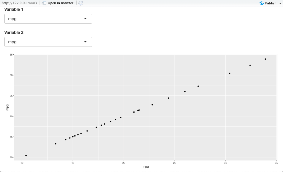
We need to “customize” it for better workflow and aesthetics.
Now, we will explore how to make your UI layouts more sophisticated and workable than just a sequence of elements.
11.3.1 Customizing Basic Layouts within a fluidPage() Function
We create basic layouts by adding arguments to the fluidPage() function.
- The arguments to
fluidPage()are functions which all together specify the UI layout of your app. - Each function has arguments with default values, and you can customize with your own choices.
- These multiple layers of nested functions allow for creative layouts (with lots of closing parentheses).
We’ll talk about grid layouts later, but to see more layouts go to:
navbarPage(): https://shiny.rstudio.com/gallery/navbar-example.htmldashboardPage(): https://rstudio.github.io/shinydashboard/
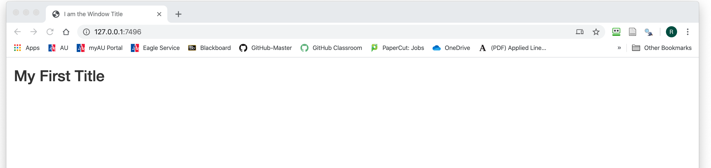
11.3.2 Add a Title Banner to Your App Using titlePanel()
This adds a title at the top of your app.
Running the app, you should get something like this:
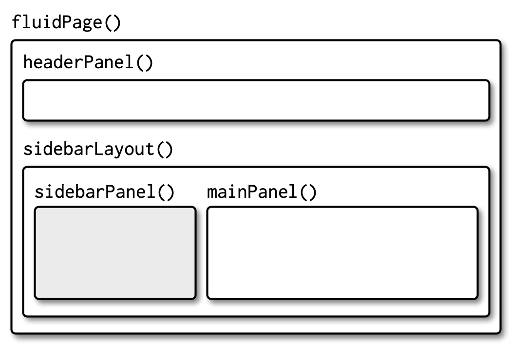
11.3.3 Create a Sidebar Layout Using sidebarLayout()
The most basic layout is a sidebar layout with a sidebar panel on the left and a main panel on the right.
- The sidebar is displayed with a distinct background color.
- The main panel occupies 2/3 of the horizontal width.
Use the function sidebarLayout() to specify this layout.
- Place it early in the
fluidPage()arguments
sidebarLayout() has two arguments sidebarPanel() and mainPanel() you can use to customize the layout of the elements within each panel:
sidebarPanel()is for input elements typically.
mainPanel()is for output elements typically.
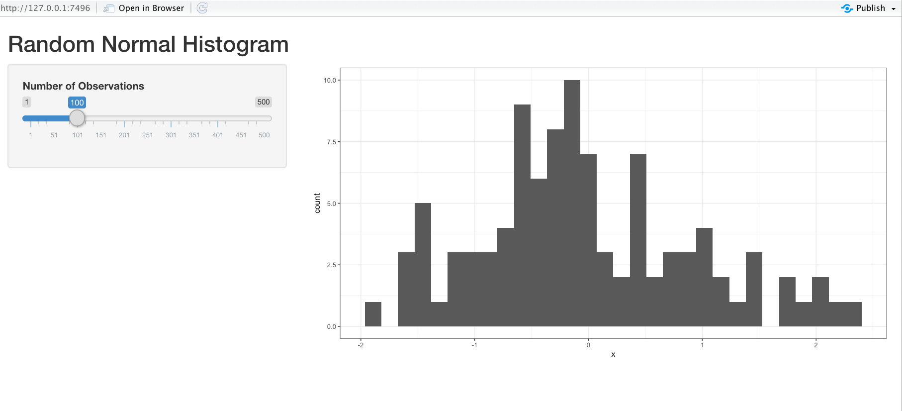
11.3.3.1 Example: Create an App with a Sidebar Layout to Plot Random Normal Draws:
Use a slider to get the number of observations and output a histogram.
library(shiny)
library(ggplot2)

ui <- fluidPage(
  titlePanel("Random Normal Histogram"),
  sidebarLayout(
    sidebarPanel(
      sliderInput("nobs", "Number of Observations",
        min = 1, max = 500, value = 100
      )
    ),
    mainPanel(
      plotOutput("hist")
    )
  )
)

server <- function(input, output) {
  output$hist <- renderPlot({
    rout <- data.frame(x = rnorm(n = input$nobs))
    ggplot(rout, aes(x = x)) +
      geom_histogram(bins = 30) +
      theme_bw()
  })
}

shinyApp(ui = ui, server = server)
Running the app, you should get something like this (side by side - not top to bottom):
11.3.4 sidebarPanelLayout() Details
sidebarPanel():
- An argument of
sidebarLayout(). - It can have arguments for input controls (elements), e.g.,
sliderInput(),textInput(), etc. - Include multiple input elements by separating them, as function arguments, with a comma.
mainPanel():
- An argument of
sidebarLayout(). - It can have arguments for output controls (elements), e.g.
plotOutput(),textOutput(), etc. - Include multiple output elements by separating them, as function arguments, with a comma.
Hadley Wickham’s graphic of a Fluid Page Layout.
You can put input elements in mainPanel() and output elements in sidebarPanel() and the app won’t die.
- UX or UI design is its own specialty.
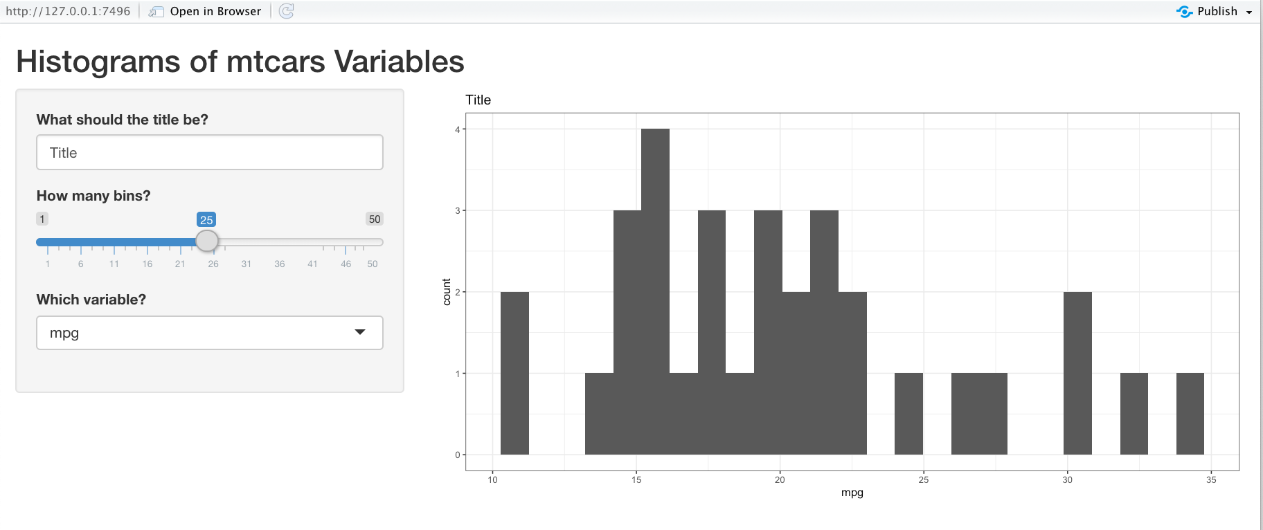
Create a Shiny app with the sidebar layout.
- The inputs should be the number of bins, the plot title, and which variable to plot from
mtcars. - The output should be a histogram.
- Add a nice shiny app title.
Show code
library(shiny)
library(ggplot2)

ui <- fluidPage(
  titlePanel("Histograms of mtcars Variables"),
  sidebarLayout(
    sidebarPanel(
      textInput("title", "What should the title be?", value = "Title"),
      sliderInput("bins", "How many bins?", min = 1, max = 50, value = 25),
      varSelectInput("var", "Which variable?", data = mtcars)
    ),
    mainPanel(
      plotOutput("plot")
    )
  )
)

server <- function(input, output) {
  output$plot <- renderPlot({
    ggplot(mtcars, aes(x = !!input$var)) +
      geom_histogram(bins = input$bins) +
      ggtitle(input$title) +
      theme_bw()
  })
}

shinyApp(ui = ui, server = server)
Your final Shiny App should look like this:
11.3.5 Create a fluidPage() Grid Layout with fluidRow() and column().
A fluidPage() layout is really a grid of rows which have columns with an assumed total browser width of 12 units
Functions fluidRow() and column() define the layout of a fluidPage().
- Rows keep their elements on the same line (if the browser has adequate width).
- Within each row,
column()allocates horizontal space within the 12-unit wide grid.
Fluid pages scale their components in real time to fill all available browser width.
fluidRow()
- Creates a new row of panels.
- The row can have a title.
- Takes
column()calls as input. - You place as many
column()calls as you want separate columns (max 12).
column()
An argument in
fluidRow().Its first argument should be a number between 1 and 12 (the
width).The sum of all
column()calls must equal 12.The rest of the arguments are input/output elements to include in a column.
Hadley Wickham’s Graphic for Fluid Page Grid Layout.
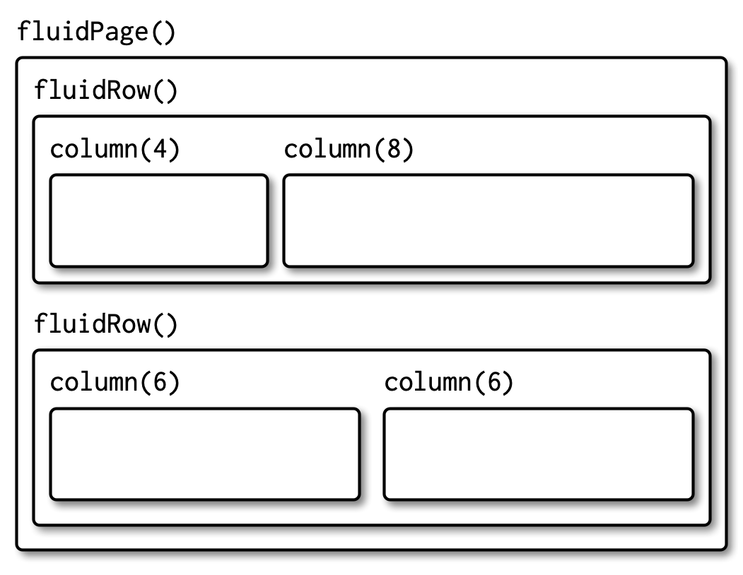
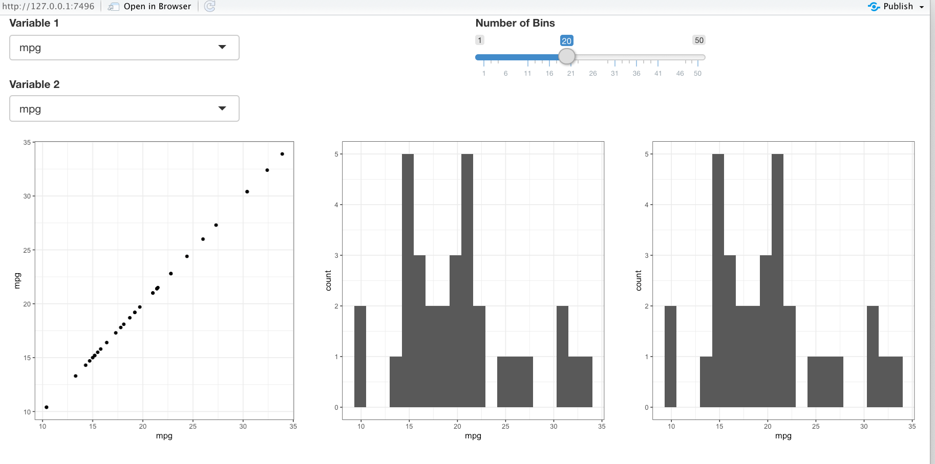
11.3.5.1 Example with fluidRow() and column()
Let’s make a shiny app to plot two variables from mtcars with two rows of panels.
- First row: two input columns: one with two inputs (variable selections) and one with one (number of bins).
- Second Row: three output columns: each with one plot: a point plot and two histograms.
library(shiny)
library(ggplot2)

ui <- fluidPage(
  fluidRow(
    column(
      6,
      varSelectInput("var1", "Variable 1", data = mtcars),
      varSelectInput("var2", "Variable 2", data = mtcars)
    ),
    column(
      6,
      sliderInput("bins", "Number of Bins",
        min = 1, max = 50, value = 20
      )
    )
  ),
  fluidRow(
    column(4, plotOutput("plot1")),
    column(4, plotOutput("plot2")),
    column(4, plotOutput("plot3"))
  )
)

server <- function(input, output) {
  output$plot1 <- renderPlot({
    ggplot(mtcars, aes(x = !!input$var1, y = !!input$var2)) +
      geom_point()
  })

  output$plot2 <- renderPlot({
    ggplot(mtcars, aes(x = !!input$var1)) +
      geom_histogram(bins = input$bins)
  })

  output$plot3 <- renderPlot({
    ggplot(mtcars, aes(x = !!input$var2)) +
      geom_histogram(bins = input$bins)
  })
}

shinyApp(ui = ui, server = server)
Running the app, you should get something like this:
Note: You can nest fluidRow()s inside fluidRow()s so it can get quite complicated.
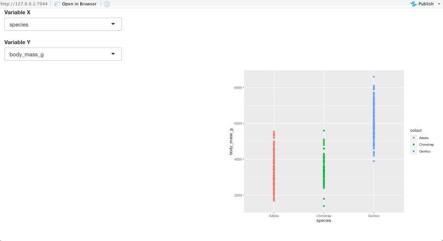
- Create a grid layout of four squares.
- Have the top left square take as input two variables of the
Palmerpenguinsdataset to include in a scatterplot. - Have the bottom right contain the resulting scatterplot, color-coded by species.
- Remember to use the unquote operator
!!for all the variables from the tibble. - The top right square and bottom left squares should remain empty.
- Have the second variable default to
body_mass_g.
- Remember to use the unquote operator
- To install
Palmerpenguins, use the following in the console:install.packages("remotes")remotes::install_github("allisonhorst/palmerpenguins")
Show code
library(shiny)
library(ggplot2)
library(palmerpenguins)

ui <- fluidPage(
  fluidRow(
    column(
      6,
      varSelectInput("var1", "Variable X", data = penguins),
      varSelectInput("var2", "Variable Y",
        selected = "body_mass_g", data = penguins
      )
    ),
    column(6)
  ),
  fluidRow(
    column(6),
    column(6, plotOutput("plot"))
  )
)

server <- function(input, output) {
  output$plot <- renderPlot({
    ggplot(penguins, aes(
      x = !!input$var1,
      y = !!input$var2,
      color = !!penguins$species
    )) +
      geom_point()
  })
}

shinyApp(ui = ui, server = server)
Your final app should look like this:
11.3.6 Creating sets of Tabs with tabsetPanel() and tabPanel()
You can subdivide layouts into tabs with tabsetPanel() and tabPanel().
Tabs can appear at multiple levels of the layout:
- At the top level of the page, or,
- In the main panel in the sidebar layout, or,
- In one of the
column()calls in the grid layout, or, - Anywhere else that makes sense.
11.3.6.1 tabsetPanel()
Use tabsetPanel() to create the placeholder for the tabs.
Arguments include calls to tabPanel() for each tab.
- You can include as many tabs as you want. If it is more tabs than fit on a line in the width of the browser, the browser will flow the tabs to create additional lines.
- The default is make the first tab active one, but you can change with the
selected =argument. - Set
type = "pills"to have the selected tab take the current background color so it is easier to see.
11.3.6.2 tabPanel()
Must be inside a call to tabsetPanel().
- The first argument is the title for the tab.
- Then add one or more input/output elements as arguments, separated by a comma, to fill the tab as desired.
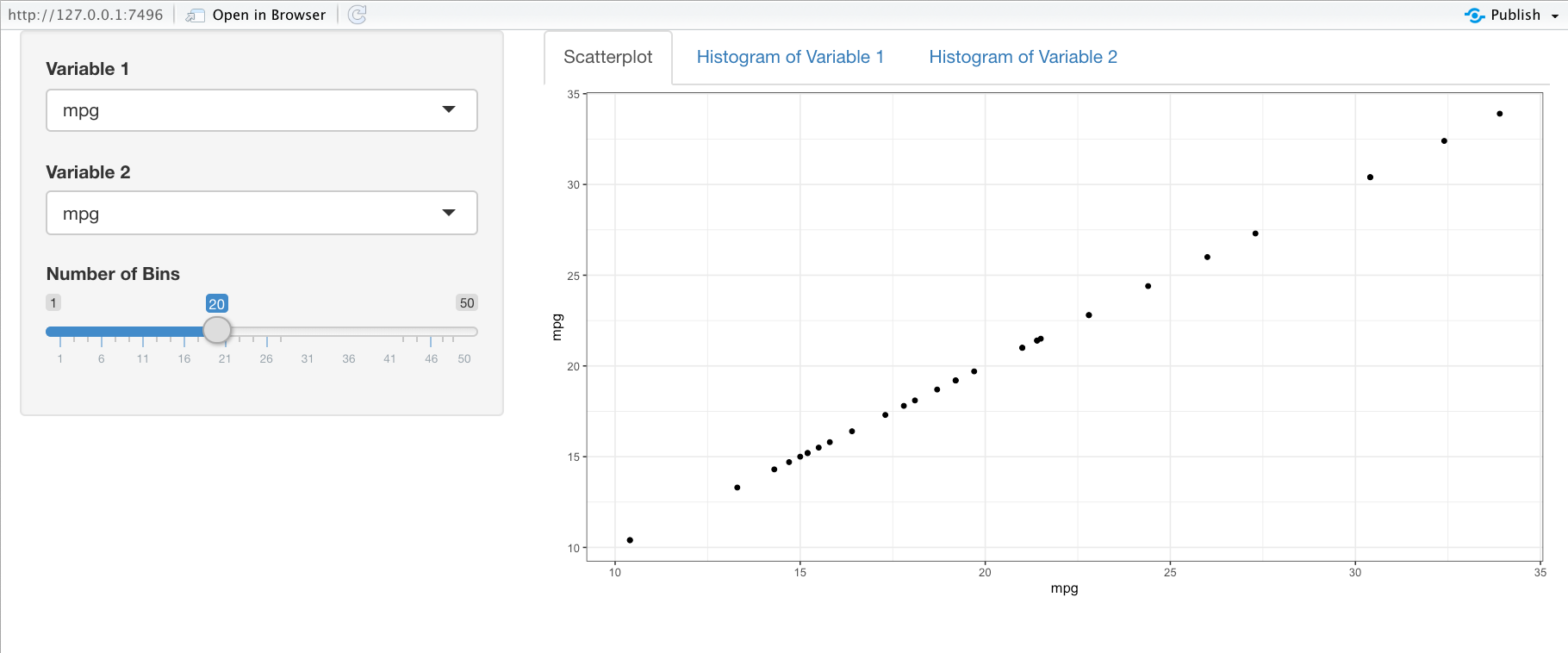
11.3.6.2.1 Example
Here is an example from the mtcars dataset, where the tabs have different plots for the variables we select.
library(shiny)
library(ggplot2)

ui <- fluidPage(
  sidebarLayout(
    sidebarPanel(
      varSelectInput("var1", "Variable 1", data = mtcars),
      varSelectInput("var2", "Variable 2", data = mtcars),
      sliderInput("bins", "Number of Bins", min = 1, max = 50, value = 20)
    ),
    mainPanel(
      tabsetPanel(
        type = "pills",
        tabPanel(
          "Scatterplot",
          plotOutput("plot1")
        ),
        tabPanel(
          "Histogram of Variable 1",
          plotOutput("plot2")
        ),
        tabPanel(
          "Histogram of Variable 2",
          plotOutput("plot3")
        )
      )
    )
  )
)

server <- function(input, output) {
  output$plot1 <- renderPlot({
    ggplot(mtcars, aes(x = !!input$var1, y = !!input$var2)) +
      geom_point()
  })

  output$plot2 <- renderPlot({
    ggplot(mtcars, aes(x = !!input$var1)) +
      geom_histogram(bins = input$bins)
  })

  output$plot3 <- renderPlot({
    ggplot(mtcars, aes(x = !!input$var2)) +
      geom_histogram(bins = input$bins)
  })
}

shinyApp(ui = ui, server = server)
Running the app, you should get something like this:
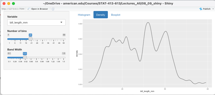
- Create a basic Shiny app with a tab for a density plot, a histogram, and a box plot for a variable from the
palmerpenguinsdataset.- The user should get to choose the variable plotted, the number of bins for the histogram, and the bandwidth for the density plot (see the help page of
geom_smooth()). - Default to bill_length_mm for the variable
- A good default value for the bandwidth might be 0.5 in this case.
- Have the second tab be the active one by default with the background color as selected
- The user should get to choose the variable plotted, the number of bins for the histogram, and the bandwidth for the density plot (see the help page of
Show code
library(shiny)
library(ggplot2)
library(palmerpenguins)

ui <- fluidPage(sidebarLayout(
  sidebarPanel(
    varSelectInput("var", "Variable",
      selected = "bill_length_mm",
      data = penguins
    ),
    sliderInput(
      "bins",
      "Number of bins",
      min = 1,
      max = 50,
      value = 20
    ),
    sliderInput(
      "bw",
      "Band Width",
      min = 0.1,
      max = 1.5,
      value = 0.5
    )
  ),
  mainPanel(tabsetPanel(
    type = "pill", selected = "Density",
    tabPanel("Histogram", plotOutput("hist")),
    tabPanel("Density", plotOutput("density")),
    tabPanel("Boxplot", plotOutput("box"))
  ))
))

server <- function(input, output) {
  output$hist <- renderPlot({
    ggplot(penguins, aes(x = !!input$var)) +
      geom_histogram(bins = input$bins)
  })

  output$density <- renderPlot({
    ggplot(penguins, aes(x = !!input$var)) +
      geom_density(bw = input$bw)
  })

  output$box <- renderPlot({
    ggplot(penguins, aes(y = !!input$var)) +
      geom_boxplot()
  })
}

shinyApp(ui = ui, server = server)
Your app should look like this:
11.3.7 Grouping Elements
11.3.7.1 Use wellPanel() to group elements together in a slightly inset border.
wellPanel()
library(shiny)
library(ggplot2)

ui <- fluidPage(
  wellPanel(
    sliderInput("bins", "How many bins?", min = 1, max = 50, value = 20),
    plotOutput("hist")
  )
)

server <- function(input, output, session) {
  output$hist <- renderPlot({
    ggplot(mtcars, aes(x = mpg)) +
      geom_histogram(bins = input$bins)
  })
}

shinyApp(ui, server)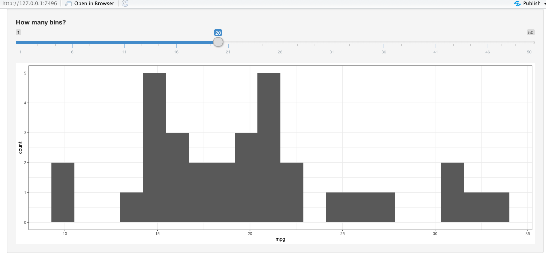
11.3.7.2 Other Panels
There are many other visual styles for groupings.
Here are some other panels for grouping elements together.
absolutePanel().conditionalPanel().fixedPanel().headerPanel().inputPanel().navlistPanel().
11.4 Customizing with Themes
Themes are defined combinations of CSS styles designed to work well together and change many aspects of the UI at once.
Bootstrap is a well established framework for creating CSS themes for many web applications (see https://en.wikipedia.org/wiki/Bootstrap_(front-end_framework%29).
- Shiny uses the classic Bootstrap v3 theme as its default so your app will not stand out with the default.
- Bootstrap Version 5 is the current version with more themes than 3 or 4. See Bootswatch
Shiny supports CSS frameworks besides Bootstrap.
You can also write your own CSS theme from scratch if you know CSS.
- The {SAAS} package allows you to use “Syntactically Awesome Style Sheets” in your app.
- See Outstanding User Interfaces with Shiny.
We will not learn CSS, but we will explore how to change and customize themes using the {bslib} package.
11.4.1 Shiny Themes with the {bslib} Package
The {bslib} package makes it easier to control main colors and fonts and/or any of the 100s of more specific theming options, directly from R.
- A significant portion of shiny UI functions have been revamped so their default styles now inherit from the overall app theme setting.
- We will see how
sliderInput(),selectInput(), anddateInput()will properly reflect the main colors and fonts of a theme.
11.4.1.1 Use bslib::bs_theme("theme_name") to Select Theme “theme_name”
You change the theme using an argument to the page layout function, e.g., as a fluidPage() argument.
- Inside
fluidPage(), set thethemeargument to bebs_theme("theme_name"), where"theme_name"is one of the themes that comes with {bslib}. - Be sure to
library(bslib)at the top of your app.
The full list of available themes can be found at Bootswatch.
- Use the console to install the {bslib} package. You may also need {reshape2}, {bsicons} and {DT} if not already installed.
- Load the {bslib} package.
Example of setting a Bootstrap 5 theme:
library(shiny)
library(ggplot2)
library(bslib)

ui <- fluidPage(
  theme = bslib::bs_theme(version = 5, bootswatch = "quartz"),
  # slate pulse, or minty, or Superhero, etc..
  titlePanel("Bootstrap Quartz"),
  sidebarLayout(
    sidebarPanel(
      sliderInput("number", "select a number", 0, 100, 40)
    ),
    mainPanel(
      tabsetPanel(
        tabPanel("a", plotOutput("hist")),
        tabPanel("b"),
        tabPanel("c")
      )
    )
  )
)
server <- function(input, output, session) {
  output$hist <- renderPlot({
    ggplot(mtcars, aes(x = mpg)) +
      geom_histogram(bins = input$number) +
      labs(title = "Sample Title")
  })
}
shinyApp(ui, server)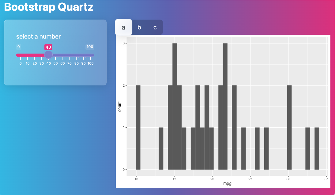
Use bs_theme_preview() to see the current theme or one of your choice.
- You can also see the colors used in each theme for the different types of elements.
- Colors are shown with their Hex Triplet and their RGB codes.
11.4.2 Use the {thematic} Package to Align {ggplot2} Themes to Match the App
The {thematic} packages simplifies theming of R graphics including {ggplot2}.
- {thematic} also enables automatic styling of R plots in Shiny, R Markdown, and RStudio.
- It also has functions for use in quarto documents being rendered to HTML.
- Load the package.
Call thematic_shiny() before launching a Shiny app to enable thematic for every plotOutput() inside the app.
- If no values are provided to
thematic_shiny(), eachplotOutput()uses the default CSS colors. - Use
thematic_shiny(font = NA)for soft synchronization of plot fonts.
# from https://rstudio.github.io/thematic/
library(shiny)
library(ggplot2)
library(thematic)

# Call thematic_shiny() prior to launching the app, to change
# R plot theming defaults for all the plots generated in the app

# Un-comment the next line to see the change
#thematic_shiny(font = NA)

ui <- fluidPage(
  theme = bslib::bs_theme(
    bg = "#002B36", fg = "#EEE8D5", primary = "#2AA198",
# bslib also makes it easy to import CSS fonts
    base_font = bslib::font_google("Pacifico")
  ),
  tabsetPanel(
    type = "pills",
    tabPanel("ggplot", plotOutput("ggplot")),
    tabPanel("lattice", plotOutput("lattice")),
    tabPanel("base", plotOutput("base"))
  )
)
server <- function(input, output) {
  output$ggplot <- renderPlot({
    ggplot(mtcars, aes(wt, mpg,
      label = rownames(mtcars),
      color = factor(cyl)
    )) +
      geom_point() +
      ggrepel::geom_text_repel()
  })
  output$lattice <- renderPlot({
    lattice::show.settings()
  })
  output$base <- renderPlot({
    image(volcano, col = thematic_get_option("sequential"))
  })
}

shinyApp(ui, server)
Example of theme Quartz with thematic_shiny(font = NA):
library(shiny)
library(ggplot2)
library(bslib)
library(thematic)
thematic_shiny(font = NA)
ui <- fluidPage(
  theme = bslib::bs_theme(version = 5, bootswatch = "quartz"),
  # slate pulse, or minty, etc..
   titlePanel("Bootstrap Quartz with `thematic_shiny()`"),
  sidebarLayout(
    sidebarPanel(
      sliderInput("number", "select a number", 0, 100, 40)
    ),
    mainPanel(
      tabsetPanel(
        tabPanel("a", plotOutput("hist")),
        tabPanel("b"),
        tabPanel("c")
      )
    )
  )
)
server <- function(input, output, session) {
  output$hist <- renderPlot({
    ggplot(mtcars, aes(x = mpg)) +
      geom_histogram(bins = input$number) +
      labs(title = "Sample Title")
  })
}
shinyApp(ui, server)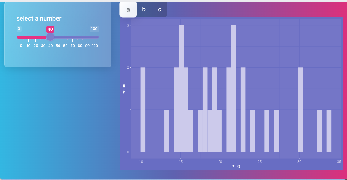
11.4.2.1 Synchronizing Plot Fonts and UI Fonts (Advanced)
- Bootstrap themes style UI text using CSS in the browser.
- R plots, e.g., {ggplot2}, base, and lattice, are rendered server-side using an R graphics device.
These are two different font systems.
- By default, {thematic} synchronizes colors between your app theme and plots.
- It does not need to synchronize fonts for your app to work correctly.
If you want color alignment but do not require identical fonts between UI and plots, the most reliable and reproducible approach is to use thematic_shiny(font = NA).
This:
- Keeps plot styling aligned with the app’s colors
- Avoids OS-specific font detection
- Prevents warnings when deploying to shinyapps.io
- Works consistently across macOS, Windows, and Linux
However, if exact font matching is required, e.g., for reasons such as branding or publication screenshots, you must explicitly synchronize fonts across:
- Bootstrap (UI) — browser-side CSS fonts
- R graphics (plots) — server-side font rendering
System fonts, e.g., Segoe UI, -apple-system, depend on the user’s operating system and may not be installed on another machine or on a deployment server.
Web fonts (especially Google Fonts) are widely used because they can be downloaded automatically by the browser and provide consistent typography across platforms. (Other hosting options exist, including privacy-focused CDNs and self-hosted fonts.)
To use the same web font in both the UI and plots, you typically combine:
- {bslib} to load the font in the browser (UI)
- {showtext} to register the font for R graphics (plots)
- {thematic} to apply the same font to plots
Example pattern (Google Font):
library(bslib)
library(showtext)
library(thematic)

FONT <- "Inter"

# Make font available to R graphics
showtext::font_add_google(FONT, family = FONT)
showtext::showtext_auto()

# Tell thematic to use it
thematic_shiny(font = FONT)

ui <- fluidPage(
  theme = bs_theme(
    version = 5,
    bootswatch = "minty",
    base_font = font_google(FONT),
    heading_font = font_google(FONT)
  )
)
This ensures consistent typography:
- Locally
- Across operating systems
- On shinyapps.io or Posit Connect
Avoid using thematic_shiny(font = "auto) for apps you want to deploy as automatic font detection depends on system-specific CSS font stacks and may produce warnings or inconsistent rendering across machines.
11.4.3 Customizing Shiny Themes with the {bslib} Package
You can use {bslib} functions to update any of the themes as well.
- See help for
bs_theme().
library(shiny)
library(ggplot2)
library(bslib)
library(thematic)
thematic_shiny(font = "auto")
ui <- fluidPage(
  theme = bs_theme(
    version = 5, bootswatch = "darkly",
    bg = "#0b3d91", # a custom blue
    fg = "white",
    base_font = "Source Sans Pro"
  ),
  sidebarLayout(
    sidebarPanel(
      sliderInput("number", "select a number", 0, 100, 40)
    ),
    mainPanel(
      tabsetPanel(
        tabPanel("a", plotOutput("hist")),
        tabPanel("b"),
        tabPanel("c")
      )
    )
  )
)
server <- function(input, output, session) {
  output$hist <- renderPlot({
    ggplot(mtcars, aes(x = mpg)) +
      geom_histogram(bins = input$number)
  })
}
shinyApp(ui, server)
11.4.4 Customizing Shiny Themes with the {fresh} Package
The {fresh} package allows you to customize Bootstrap themes in great detail.
- It is built on top of the {saas} package.
{fresh} package functions only work in an app.R file for a Shiny App.
- They won’t work inline in an R Markdown document.
11.4.4.1 Place customizations in a create_theme() call.
create_theme() arguments you should use include:
theme: What theme do you wish to customize? Say"default"for the default Shiny theme.- Otherwise, say one of the themes from the shinythemes package, see
help("shinythemes").
- Otherwise, say one of the themes from the shinythemes package, see
output_file: The location to put the customized formatting file. This should end with “.css” since it will be a CSS file.- For now, you must place the output file in a “www” sub-directory of the folder your Shiny App
app.Rfile is in.
Every other argument of create_theme() starts with bs (for bootstrap), e.g., a variant of bs_vars_*().
- For example,
bs_vars_global()adjusts the global environment of the Shiny App (default text color, background color, the presence of a border, etc).
You can get those hexadecimal colors by either searching for “color wheel” or looking up the common web colors: http://websafecolors.info/color-chart.
In fluidPage(), you then give the theme argument the path to the CSS file.
- You don’t need to say “www/mytheme.css” since Shiny will make the contents of the
wwwdirectory available in the working directory.
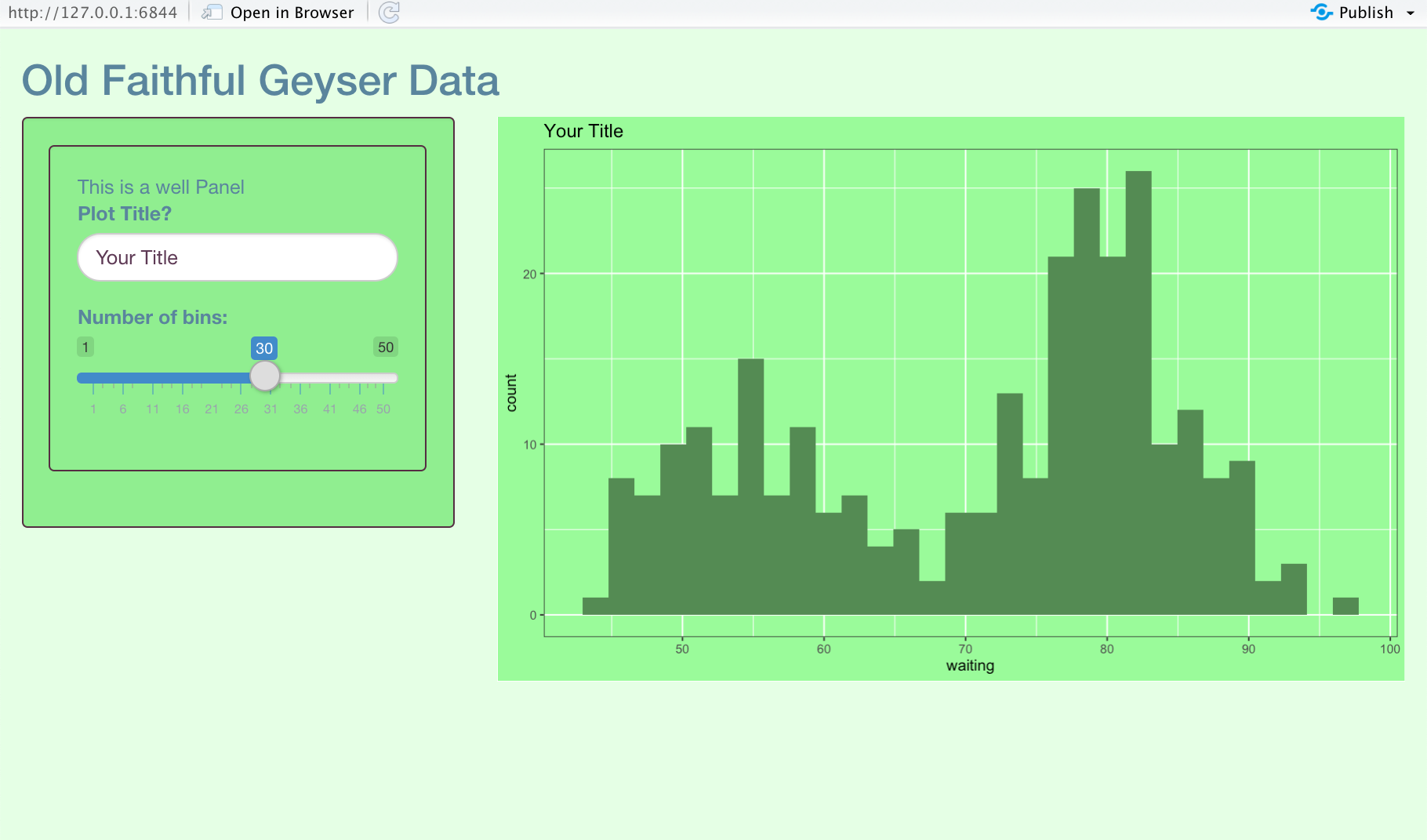
11.4.4.2 Example of Changing the Background Colors
Copy and paste into an app.R file.
library(shiny)
library(shinythemes)
library(fresh)
library(ggplot2)

create_theme(
  theme = "default",
  bs_vars_color(
    gray_base = "#354e5c"
  ),
  bs_vars_wells(
    bg = "#90ee90",
    border = "#552D42"
  ),
  bs_vars_global(
    body_bg = "#e5ffe5"
  ),
  bs_vars_input(
    color = "#5d3954",
    border_radius = "20px"
  ),
  #
  output_file = "www/mytheme.css"
)

ui <- fluidPage(
  theme = "mytheme.css",
  titlePanel("Old Faithful Geyser Data"),
  sidebarLayout(
    sidebarPanel(
      wellPanel(
        "This is a well Panel",
        textInput("plot_title", "Plot Title?", value = "Your Title"),
        sliderInput("bins",
          "Number of bins:",
          min = 1,
          max = 50,
          value = 30
        )
      )
    ),
    mainPanel(
      plotOutput("distPlot")
    )
  )
)

server <- function(input, output) {
  output$distPlot <- renderPlot({
    ggplot(faithful, aes(x = waiting)) +
      geom_histogram(bins = input$bins, fill = "palegreen4") +
      theme(plot.background = element_rect(fill = "palegreen1")) +
      ggtitle(input$plot_title) +
      theme(
        panel.background = element_rect(
          fill = "palegreen1",
          color = "palegreen1",
          size = 0.5, linetype = "solid"
        ),
        panel.grid.major = element_line(
          size = 0.5, linetype = "solid",
          color = "white"
        ),
        panel.grid.minor = element_line(
          size = 0.25, linetype = "solid",
          color = "white"
        )
      )
  })
}

shinyApp(ui = ui, server = server)
Inline (you must have a www folder at the level of your .Rmd file).
- notice no change in background.
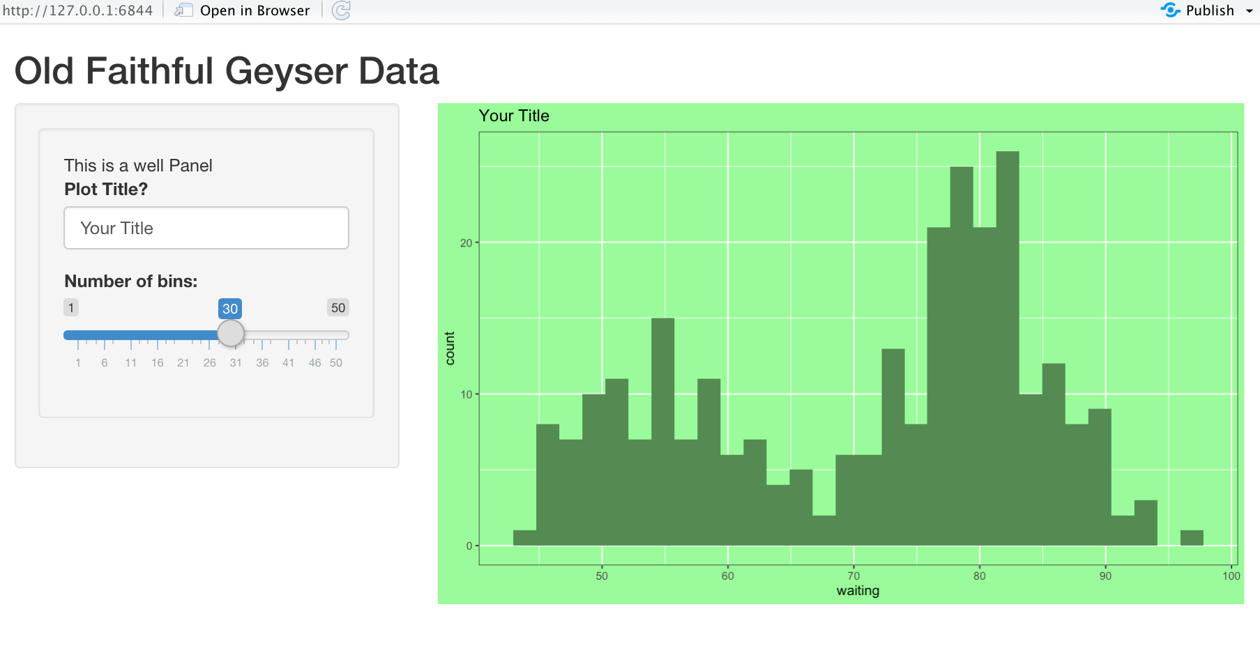
- As a separate app you can see the change in background
11.5 Using HTML in Shiny Apps
HTML (Hypertext Markup Language) is a coding language like R markdown used to structure and style web documents (in conjunction with CSS).
- When you look at a web page, that is a browser interpreting the HTML code.
The {shiny} package functions allow you to use R to create the HTML for the user interface without having to learn or write raw HTML.
11.5.1 HTML Basics
Elements surrounded by “<>” are called HTML “tags”.
Use tags in pairs, with a beginning <tag> and an ending </tag> with a forward slash in it.
For example:
<strong>...</strong>: Makes text bold. Sesquipedalian<u>...</u>: Makes text underlined. Sesquipedalian<s>...</s>: Makes text strikeout.Sesquipedalian<code>...</code>: Makes text mono-spaced.Sesquipedalian<br></br>: Inserts a line break.
Some text
More text
<hr></hr>: Inserts a horizontal “rule” (line).
<h1>...</h1>,<h2>...</h2>,<h3>...</h3>: Creates headings, subheadings, sub-subheadings.Sesquipedalian
Sesquipedalian
Sesquipedalian
<p>...</p>: Makes paragraphs.Here is a new paragraph Sesquipedalian
- The following creates an un-numbered list with two list items:
- Item 1
- Item 2
<img></img>: Inserts images (see below).<a>...</a>: The “anchor” tag. Creates hyperlinks (see below).
11.5.1.1 Tag Attributes are Arguments
Tag “attributes” are entered as arguments and are placed after the tag name in the first <>.
- As an example, the
atag for hyperlinks requires anhrefattribute with a URL or hypertext reference. - You can also add text to be displayed for the link, here “Click Me!”.
<a href="https://www.youtube.com/watch?v=Nnuq9PXbywA">Click Me!</a>This yields:
- The image tag
imgrequires asrcattribute for the source of the image.
This yields:
![]()
11.5.3 Using HTML in a Shiny App
- To use HTML elements in your Shiny UI, put them inside the call to
fluidPage()using thetags().
Use the img tag to insert the American University logo into a Shiny App.
- The url can be found here: https://upload.wikimedia.org/wikipedia/commons/c/c6/American_University_logo.svg
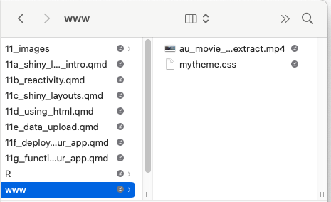
11.5.3.1 Adding Images or Videos Not from a Web Page
To add an image (or video) not from a web page, add a www folder inside your Shiny app in your R folder.
- Put all the images or videos into that folder.
- Reference those images by name only (not by the path) in the
imgtag.
Note: This can’t be run in a code chunk. It must be a separate app file in its own directory.
library(shiny)
ui <- fluidPage(
  tags$img(src = "AU-Logo-on-white-small.png"),
  wellPanel(
    h1("AU Website Video"),
    br(),
    h5("Open in a browser"),
    hr(),
    tags$video(
      width = "100%", type = "video/mp4", controls = NA,
      autoplay = TRUE, muted = FALSE, loop = NA,
      src = "au_movie_am_low_extract.mp4"
    )
  )
)

server <- function(input, output, session) {
}

shinyApp(ui, server)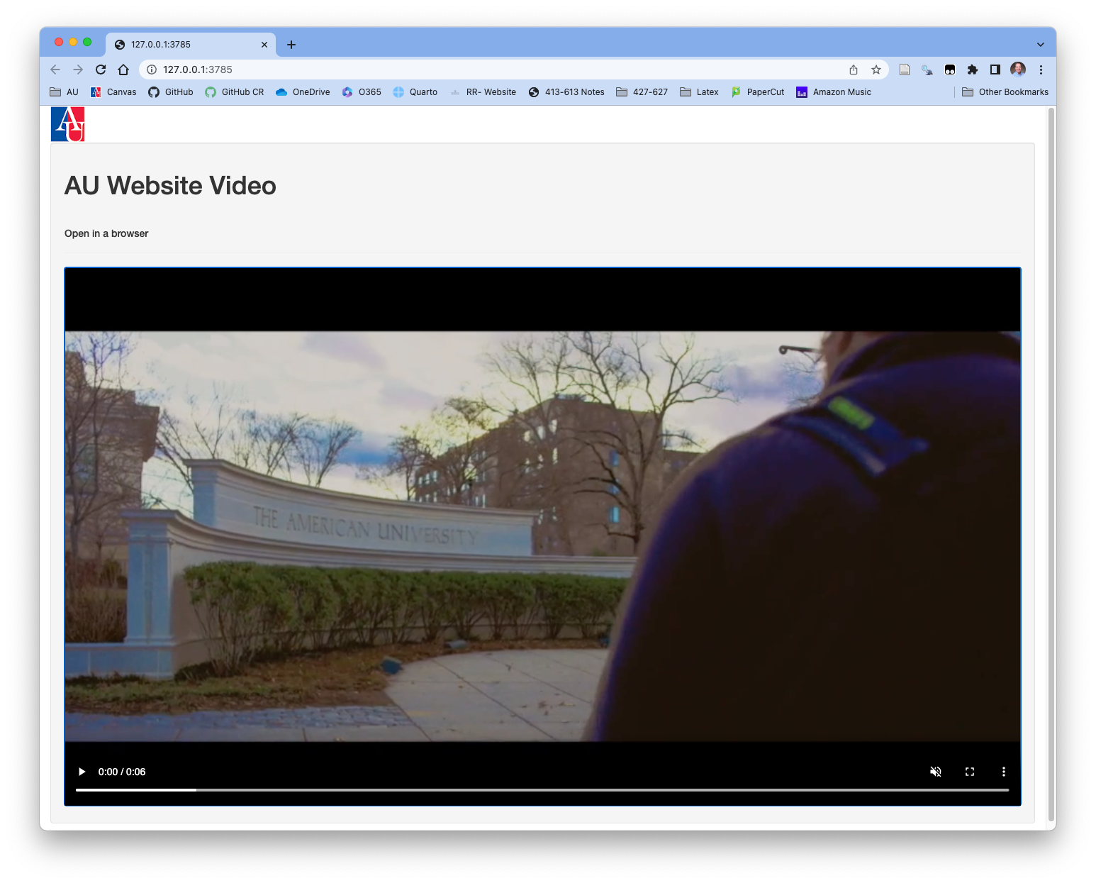
11.5.3.2 Adding Text with HTML Tags
If you want to add a lot of text to an app you can use the ptag.
Entering the following:
  tags$div(
      tags$p("First paragraph"),
      tags$p("Second paragraph"),
      tags$p("Third paragraph")
  )
generates
   <div>
      <p>First paragraph</p>
      <p>Second paragraph</p>
      <p>Third paragraph</p>
</div> It’s fine to use the tags for short bits of text in your app.R file.
However, for longer sections of text or multiple paragraphs of text, it is much better to treat it as “data” that you can edit and configuration manage outside your app.R file.
Create a file with tags that you source() in the appropriate place in the ui.
- You can use all the same tags for structure and arguments for attributes and formatting.
- Be sure to use the
local = TRUEargument when yousource().
Either way will work, but it is generally much easier to manage large blocks of text in a separate file. It also makes your app.R much cleaner and easier to work with as well.
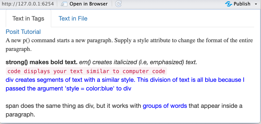
library(shiny)
ui <- fluidPage(
tabsetPanel(
tabPanel(
"Text in Tags",
tags$a("Posit Tutorial", href = "https://shiny.posit.co/r/getstarted/shiny-basics/lesson2/"),
p("A new p() command starts a new paragraph. Supply a style attribute to change the format of the entire paragraph.", style = "font-family: 'times'; font-si16pt"),
strong("strong() makes bold text."),
em("em() creates italicized (i.e, emphasized) text."),
br(),
code("code displays your text similar to computer code"),
div("div creates segments of text with a similar style. This division of text is all blue because I passed the argument 'style = color:blue' to div", style = "color:blue"),
br(),
p(
"span does the same thing as div, but it works with",
span("groups of words", style = "color:blue"),
"that appear inside a paragraph."
)
),
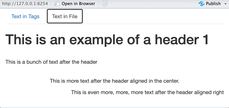
tabPanel(
"Text in File",
source("./R/shiny_upload_textfile.R", local = TRUE)$value
)
)
)
server <- function(input, output, session) {
}
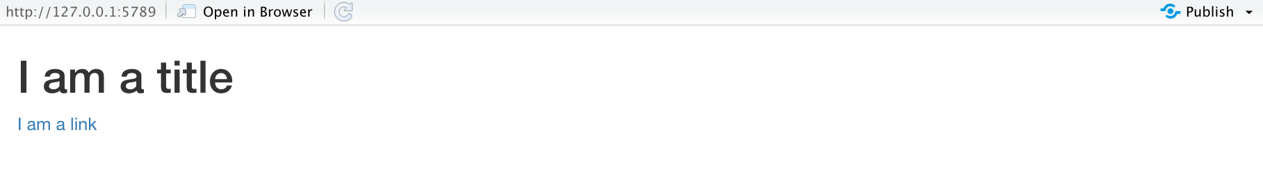
shinyApp(ui, server)The file that read in by source()looks like the following:
[1] "tags$div("
[2] "  h1(\"This is an example of a header 1\"),"
[3] "  br(),"
[4] "  p(\"This is a bunch of text after the header\"),"
[5] "  br(),"
[6] "  p(\"This is more text after the header aligned in the center.\", align = \"center\"),"
[7] "  p(\"This is even more, more, more text after the header"
[8] "    aligned right\", align = \"right\")"
[9] ")"
The two panels of app look like:
11.5.4 HTML Widgets
HTML widgets for R produce interactive web visualizations in HTML documents like web pages or shiny apps.
- Widgets are popular with HTML developers as they allow users to embed high quality “mini apps”s in their code without having to code them.
- After loading the widget library, you can use just a few lines of code to create a variety of interactive displays in your HTML.
- HTML widgets can be used at the R console as well as embedded in quarto reports and Shiny web applications.
- As the title suggests - they don’t work in PDF documents.
There are over 100 widgets on the R site.
- Widgets are a huge time saver but can be a huge time black hole.
- We’ll look at three popular ones:
plotly,rpivotTable, andtmap.
11.5.4.1 The {plotly} package is a popular interactive graphics extension to {ggplot2}
- Load the {ggplot2} and {plotly} libraries.
- Create a plot with
ggplot(). - Call
ggplotly(myplot)to make it interactive.
Example with the diamonds data from ggplot2.
{plotly} comes with its own output type and render functions in Shiny.
plotlyOutput()creates the space for the widget in your layout.renderPlotly()creates the HTML for a plot.
11.5.4.2 An Excel-like Pivot Table Widget
Pivot Tables have been called one of the “magical features” of spreadsheets and may often be desired by folks wanting to explore your data.
-This package includes by numerical summaries and pivot charts
The pivot table widget requires two packages: htmlwidgets and rpivotTable
- Use
devtools::install_github(c("ramnathv/htmlwidgets", "smartinsightsfromdata/rpivotTable"))in the console. - You may need to update other packages and can say no to the question Do you want to install from sources the package which needs compilation? (Yes/no/cancel).
- Load the {rpivotTable} package.
- Use your tibble as an argument to
rpivotTable(). - Drag and Drop the fields as you might on an Excel Pivot table and adjust the calculations as desired.
Let’s do an example with the Palmer Penguins data.
- If needed, enter
remotes::install_github("allisonhorst/palmerpenguins")in the console.
{rpivotTable} comes with its own output type and render functions in Shiny.
rpivotTableOutput()creates the space for the widget in your layout.renderRPivotTable()creates the HTML for the widget.
11.5.4.3 The {tmap} Package: an HTML Widget for Creating Thematic Maps
Thematic maps are geographical maps on which spatial data distributions have been layered.
The {tmap} package offers a flexible, layer-based, and easy to use approach to create thematic maps, such as choropleths and bubble maps.
- See the Get Started! vignette
- Use the console to install the package {tmap} from CRAN.
- Load the library {tmap}.
- Load your data.
- Use the desired functions to generate the map.
Each map can be plotted as a static image or viewed interactively using “plot” and “view” modes, respectively.
- The mode can be set with the function
tmap_mode() - Toggling between the modes can be done with the ‘switch’
ttm()(which stands for toggle thematic map). - {tmap} has many different functions and arguments to customize your map.
{tmap} comes with its own output type and render functions in Shiny.
tmapOutput()creates the space for the widget in your layout.renderTmap()creates the HTML for the widget.- Note: {tmap} cannot do everything in Shiny that it can do in static HTML documents, e.g., facet.
library(shiny)
library(tmap)
data(World) # data frame with multiple data fields  and geographic data

ui <- fluidPage(
  tmapOutput("map", height = 800)
)

server <- function(input, output, session) {
  output$map <- renderTmap({
    tmap_mode("view")
    tm_shape(World) +
      tm_polygons(col = "life_exp")
  })
}

shinyApp(ui, server)
11.6 Uploading Data into Shiny
11.6.1 Uploading Static Datasets
If your Shiny app is designed to analyze only a single known dataset (which might contain multiple files), then you should upload the data at the start of the app.
- Create a
\datafolder in your app structure. - Place all data files in the
\datafolder. - Read in the data files in the business logic section.
For speed with large data or data that requires a lot of pre-processing, do the following:
- Save the original data in a
\data-rawfolder. - Write R scripts in the
\data_rawfolder to pre-process the data and usereadr::write_rds()in the script to save the data frame (possibly using thecompress =argument) with extension.Rdsinto the separate\datafolder. - Then you can use
readr::read_rds()to be faster on start up by avoiding the pre-processing of the data. - You could also use
save()andload()to save multiple objects (use extension.Rdata) but you have to use the names as stored as you can’t reassign RData objects to different variable names when you load them.
As an example:
- Read the
estate.csvfile in from https://raw.githubusercontent.com/AU-datascience/data/main/413-613/estate.csv and save as an.rdsfile usingwrite_rds().
- Load the
.rdsdata at beginning of the app in the business logic section.
When a shiny app is run, the location of app.R is the working directory, so all file upload/download must be done using a relative path from that directory.
Quarto files with inline shiny code chunks operate from the Quarto file working directory, i.e., were the file is saved.
11.6.2 Upload Data Files Interactively with fileInput().
Use the fileInput() function in the UI to allow users to choose the source of the data set.
- It opens up the computer’s default file browser.
The input object (here input$file) is not the data but a data frame with the following columns:
name: The name of the file on the user’s computer.size: The size of the file in bytes. Shiny only accepts files up to 5 MB by default.type: The file extension (text/csv, text/plain, etc.).datapath: A temporary path file.
fileInput has several arguments for adjusting its behavior:
accept: What file extensions are acceptable (".csv",".txt", etc.).buttonLabel: Customize label of button.multiple: Set =TRUEto allow users to select and upload multiple files at once. This does not work on older browsers, including Internet Explorer 9 and earlier.
Here is an example with optional arguments.
The files are NOT read in when selected and will not appear in the environment.
The UI fileInput() allows the user to select multiple file names and identifies where they are.
The reactive element code in the server side actually reads in the selected files.
Place the code to access the data in the selected files in a reactive() function or you can load inside a render*() if you only need the data in that one place.
- In the server function, use the
datapathvalue as thepathargument inread_csv(),read_tsv(),readRDS(), etc.. - Before the line loading the data, use
req()so Shiny waits for the user’s choice before executing the code to access the data files listed in theinput$filedata frame. - Save the read-in data to a variable and note the variable will be a reactive element so requires the
()when used.
If the files are Not the same structure, they can’t go into the same tibble without some manipulation unless you are nesting them.
In that case, read the in one at a time.
11.6.3 Increasing the Default File Size Limitation in Shiny
For fileInput(), Shiny enforces a default upload limit of 5MB for a file.
Shiny has a parameter you can set to increase the default limit on file upload size.
- To increase it to XX MB, where
XXis a number, type the following in the business logic section inapp.R:options(shiny.maxRequestSize = XX * 1024^2). - The limitation is the size of the temporary disk space for the data.
This example shows a 50MB file uploads into Shiny.
library(shiny)
library(rvest)
library(tidyverse)
library(stringr)

options(shiny.maxRequestSize = 60 * 1024^2)
file_name <- "BPD_Part_1_Victim_Based_Crime_Data.csv"
input_path <- "https://raw.githubusercontent.com/AU-datascience/data/main/413-613/BPD_crime_files/"

bpd <- read_csv(str_c(input_path, file_name, sep = ""))

ui <- fluidPage(
  verbatimTextOutput("summ")
)

server <- function(input, output, session) {
  output$summ <- renderPrint(summary(bpd))
}

shinyApp(ui, server)The option options(shiny.maxRequestSize = ...) applies only to files uploaded by users via fileInput().
It does not limit the size of data files that your app reads directly from disk or from a URL.
11.6.4 Using Parquet Format for Larger Datasets
If your data set is moderately large, you can store the data in a compressed binary format such as parquet which is shareable across different languages (unlike .rds)
- Parquet files are significantly smaller than CSV files, they load faster and they preserve column types.
- Saving in parquet format can simplify your workflow (no need to split and recombine files)
A common pattern is to preprocess the data once and store a parquet version in your app’s /data directory.
The following example uses data downloaded from the Baltimore Police Department crime data.
- The Baltimore Police Department provides a large CSV file of crime data. Rather than splitting the file, you can convert it once to parquet and reuse it in your app.
Step 1: Use the {arrow} package to convert CSV to Parquet (outside the app)
library(readr)
library(arrow)
library(stringr)

# File information
file_name <- "BPD_Part_1_Victim_Based_Crime_Data.csv"
input_path <- "https://raw.githubusercontent.com/AU-datascience/data/main/413-613/BPD_crime_files/"
output_path <- "./data/"

# Read the CSV from the remote source
crime_df <- read_csv(str_c(input_path, file_name))

# Write to parquet in the app's data directory
write_parquet(
  crime_df,
  sink = str_c(output_path, "bpd_crime.parquet")
)
Step 2: Use the Parquet File in Your Shiny App
11.6.5 Options for Very Large Data: Partitioning and GitHUb Large File System
11.6.5.1 Partitioning Data with Parquet
For even larger data sets, you can go beyond a single parquet file and store the data as a partitioned dataset.
- This splits the data into multiple parquet files organized by a discrete variable such as year, state, or category.
Partitioning allows you to only read in the relevant partitions of the data when you need them, which can significantly improve performance.
Thus, partitioning
- improves read performance (only relevant partitions are scanned)
- keeps files at manageable sizes
- mirrors how modern data systems (e.g., Spark, DuckDB, cloud warehouses) store data
Example: Partition Baltimore Crime Data by Year
- Instead of writing one file, we choose a name for the folder to hold the partitioned data and create the partitioned dataset under the
/datadirectory.
Step 1: Create Partitioned Parquet Dataset
- In this case we could use
DISTRICTbut it seems to make more senses for the analysis to create a variableyearto use as the partitioning variable.
library(readr)
library(dplyr)
library(arrow)
library(stringr)
library(lubridate)

# File information
file_name <- "BPD_Part_1_Victim_Based_Crime_Data.csv"
input_path <- "https://raw.githubusercontent.com/AU-datascience/data/main/413-613/BPD_crime_files/"
output_path <- "data/bpd_crime_dataset"

# Read data
crime_df <- read_csv(str_c(input_path, file_name))

# Create a year variable (adjust column name if needed)
crime_df <- crime_df |>
  mutate(year = year(as.Date(CrimeDate)))

# Write partitioned parquet dataset
write_dataset(
  crime_df,
  path = output_path,
  format = "parquet",
  partitioning = "year"
)- The
data/bpd_crime_datasetdirectory now has sub-directories for each year with files that are about 500K.
data/
└── bpd_crime_dataset/
    ├── year=2018/
    │   └── part-0.parquet
    ├── year=2019/
    │   └── part-0.parquet
    ├── year=2020/
    │   └── part-0.parquet
    └── ...
Step 2: Read the Partitioned Dataset in Shiny
When you filter on a partition variable (like year), Arrow will:
- skip reading unrelated files entirely
- dramatically reduce I/O and memory usage
This is called partition pruning and is a key performance optimization in modern data systems.
Use a partitioned dataset when:
- the data is large (tens of MBs and up)
- you frequently filter by a variable (e.g., year, state)
- you want faster app performance
Avoid “over-partitioning” (e.g., by a high-cardinality variable like ID), which can create too many small files.
11.6.5.2 GitHub Large File Storage (LFS)
If your data file exceeds GitHub’s 100 MB limit, it will not allow you to push it to a normal repo.
If you need to store it, and for free accounts it is less than 2GB, you can use GitHub Large File Storage (LFS) GitHub LFS to version them.
At a high level, the workflow is:
- Install Git LFS on your system and initialize it for your repository.
- Configure tracking for the file types you want Git to manage (e.g., .parquet, .csv).
- Add and commit your files as usual—Git LFS will store the large file contents separately and keep lightweight pointers in the repository.
- Push to GitHub, where the large files are stored via LFS rather than the standard Git object store.
Keep in mind that GitHub LFS has storage and bandwidth limits, especially on free plans, so it is best suited for moderately large data rather than very large or frequently updated datasets.
If you accidentally commit a file larger than 100 MB, GitHub will reject the push, even if you delete the file afterward as the file (blob) remains in the repository’s history.
To fix this, you must rewrite the Git history to remove the file completely.
The recommended approach is to use the BFG Repo-Cleaner which removes large files (or other data you might want to remove) from all commits.
After cleaning the history, you will need to force push the repository to GitHub.
Be aware that rewriting history can affect collaborators, so this is easiest to do before others have cloned or based work on the repository.
11.6.6 Using {readr} to Read in Multiple Files where the Files have the Same Variable (column) Structure.
The {readr} package uses the {vroom} package for speed in loading delimited and fixed-width files.
- {vroom} uses lazy evaluation to create an index of the data and then it loads the actual data only if needed.
Assume you have multiple files with the same variable/column structure and similar names.
We can use the {fs} package to help create a variable with our file names by searching the directory where they are located (simplified below so only those files are in that directory).
- Then we can efficiently read them into one tibble by passing the file names directly to
readr::read_csv()`. - In this example, the data came as set of files of 9MB each.

readr::read_csv()reads the list of file names into a single tibble with 344K rows.
We can use the same capabilities in Shiny.
Assume you want the user to select and input multiple files with a common structure and naming convention.
- Using
input$file$datapathinsideread_csv()will load all the files and bind them by rows to get a single tibble.
If you have multiple files with different structures, you can use the individual elements of input$file$datapath to load the files individually.
The following allows the user to chose one or more files from the set of Baltimore PD Crime files.
- Since Shiny does not know what the data looks like when it starts (
data=is set tocharacter(0))), the following usesobserve()withbind_event()andupdateSelectInput()to change the variable names available for thevarSelectInput()elements. - This method is described in more detail in Mastering Shiny: Dynamic UI.
library(shiny)
library(readr)
library(dplyr)
library(ggplot2)
library(lubridate)

options(shiny.maxRequestSize = 10 * 1024^2)
# only set up for multiple files with the same columns.
#
ui <- fluidPage(
  sidebarLayout(
    sidebarPanel(
      fileInput("file", "What file(s)?",
        accept = "text/csv", multiple = TRUE
      ),
      varSelectInput("dfx", "Select categorical X variable", data = character(0)),
      varSelectInput("dfy", "Select variable for counts", data = character(0)),
      checkboxInput("logdata", "Log Y Scale?")
    ), # sidebarPanel
    mainPanel(
      plotOutput("boxp"),
      verbatimTextOutput("summ")
    ) # mainPanel
  ) # sidebarLayout
) # fluidPage

server <- function(input, output, session) {
  df <- reactive({
    req(input$file)
    read_csv(input$file$datapath) |>
      mutate(CrimeDate = mdy(CrimeDate),
             c_day = day(CrimeDate),
             c_dow = wday(CrimeDate, label = TRUE),
             c_month = month(CrimeDate, label = TRUE)
    ) |>
      select(c_day, c_dow, c_month, Description, 'Inside/Outside',
             Weapon, District)
  })

  observe({
    updateVarSelectInput(session, "dfx", data = df(), selected = "Weapon")
  }) |>
    bindEvent(df())

   observe({
    updateVarSelectInput(session, "dfy", data = df())
  }) |>
    bindEvent(df())

  df2 <- reactive({
    df() |>
      select(!!input$dfx, !!input$dfy) |>
      group_by(!!input$dfx, !!input$dfy) |>
        summarize(total = n())
  })


  output$summ <- renderPrint({
    summary(df2())
  })

  output$boxp <- renderPlot({
    p <- ggplot(df2(), aes(x = !!input$dfx, y = total)) +
      geom_boxplot()
    if (input$logdata) {
      p <- p + scale_y_log10()
    }
    p
  }) # renderPlot
}

shinyApp(ui, server)
If you were to use the debugging tools on the above app, e.g., insert browser() right after the req() line, you could see the datapaths for six selected files looks like the following. It shows the “temporary” location where shiny puts the data to load it.
input$file$datapath [1] "/var/folders/_7/4_9z3s852cng3ktlr0pvn99h0000gn/T//RtmpmLmojY/9af03c9260120971047310ed/0.csv" [2] "/var/folders/_7/4_9z3s852cng3ktlr0pvn99h0000gn/T//RtmpmLmojY/9af03c9260120971047310ed/1.csv" [3] "/var/folders/_7/4_9z3s852cng3ktlr0pvn99h0000gn/T//RtmpmLmojY/9af03c9260120971047310ed/2.csv" [4] "/var/folders/_7/4_9z3s852cng3ktlr0pvn99h0000gn/T//RtmpmLmojY/9af03c9260120971047310ed/3.csv" [5] "/var/folders/_7/4_9z3s852cng3ktlr0pvn99h0000gn/T//RtmpmLmojY/9af03c9260120971047310ed/4.csv" [6] "/var/folders/_7/4_9z3s852cng3ktlr0pvn99h0000gn/T//RtmpmLmojY/9af03c9260120971047310ed/5.csv"
11.6.6.1 Reading Compressd File Types such as Zip and Gz
The {read_csv} and {vroom} packages also support reading zip, gz, bz2, and xz compressed files automatically.
- Just use the path/file name of the compressed file as the argument.
- For remote files (a URL),
vroom()only works with.gzfiles.
Rows: 32
Columns: 12
$ model <chr> "Mazda RX4", "Mazda RX4 Wag", "Datsun 710", "Hornet 4 Drive", "H…
$ mpg   <dbl> 21.0, 21.0, 22.8, 21.4, 18.7, 18.1, 14.3, 24.4, 22.8, 19.2, 17.8…
$ cyl   <dbl> 6, 6, 4, 6, 8, 6, 8, 4, 4, 6, 6, 8, 8, 8, 8, 8, 8, 4, 4, 4, 4, 8…
$ disp  <dbl> 160.0, 160.0, 108.0, 258.0, 360.0, 225.0, 360.0, 146.7, 140.8, 1…
$ hp    <dbl> 110, 110, 93, 110, 175, 105, 245, 62, 95, 123, 123, 180, 180, 18…
$ drat  <dbl> 3.90, 3.90, 3.85, 3.08, 3.15, 2.76, 3.21, 3.69, 3.92, 3.92, 3.92…
$ wt    <dbl> 2.620, 2.875, 2.320, 3.215, 3.440, 3.460, 3.570, 3.190, 3.150, 3…
$ qsec  <dbl> 16.46, 17.02, 18.61, 19.44, 17.02, 20.22, 15.84, 20.00, 22.90, 1…
$ vs    <dbl> 0, 0, 1, 1, 0, 1, 0, 1, 1, 1, 1, 0, 0, 0, 0, 0, 0, 1, 1, 1, 1, 0…
$ am    <dbl> 1, 1, 1, 0, 0, 0, 0, 0, 0, 0, 0, 0, 0, 0, 0, 0, 0, 1, 1, 1, 0, 0…
$ gear  <dbl> 4, 4, 4, 3, 3, 3, 3, 4, 4, 4, 4, 3, 3, 3, 3, 3, 3, 4, 4, 4, 3, 3…
$ carb  <dbl> 4, 4, 1, 1, 2, 1, 4, 2, 2, 4, 4, 3, 3, 3, 4, 4, 4, 1, 2, 1, 1, 2…
11.7 Deploying your App
If you want others to see your App when you are not running it yourself, you can deploy it onto a server.
Shinyapps.io is a shiny server hosting service provided by the Posit organization.
- The service allows anyone to deploy a shiny app to their shiny servers where it will be accessible to the public.
Posit offers several tiers of pricing to include a Free tier.
- The free tier allows up to five applications at once and a total of 25 “Active Hours” per month.
- Active hours are hours where your application is “not idle.”
- If you exceed them, the access will be suspended until the next month unless you upgrade to the next tier.
11.7.1 Get a shinyapps.io Account
Go to shinyapps.io and click “Sign Up”.
- The site will give you several options for signing in.
- If you have a Google account or a GitHub account, you can use either one of those methods to authenticate.
- Alternatively you can create a username/password combination.
The first time you sign in, shinyapps.io prompts you to set up your account.
- shinyapps.io uses the account name as the domain name for all of your apps.
- Account names must be between four and 63 characters and can only contain letters, numbers, and dashes (-).
- Account names may not begin with a number or a dash, and they cannot end with a dash.
- They must be unique and not one of the reserved names.
11.7.2 Ensure Your App is Working and in a separate RStudio Project
Ensure the app.R file is at the top level of the directory.
Run the app locally to ensure it is working. Close the app.
If it is not already its own project, create an RStudio Project just for the app directory.
- The
app.Rmust be in its own project and GitHub repo and not inside an existing RStudio Project or GitHub repository with anything else. - Recommend setting up the project with Git and GitHub - it can be a private repo on GitHub.
- The main branch will be your “production version” you want to deploy.
- You use git branches (or a separate repo) for working on updates to the app.
11.7.3 Configure the {rsconnect} Package and Shinyapps.io Tokens
shinyapps.io automatically generates a token and secret for you.
- Retrieve your token from the shinyapps.io dashboard by selecting the Tokens option in the menu at the top right of the shinyapps dashboard (under your avatar).
- You can save these to your credential manager using the
keyring::key_set()function.
The {rsconnect} package will use your token and secret to access your account.
- Use the console to install/update the {rsconnect} package.
Once you have installed the {rsconnect} package and saved your token and secret, you can use the RStudio Tools/Global Options to configure your account.
- Open the
Tools/Global Options, selectPublishing, and follow the steps beginning with logging into your shinyapps.io account. - As an alternative, you can also use the following command to configure the {rsconnect} package to use your token and secret to access your account.
- Change the names for the token and secret to match what you used for your credential manager with
keyring::key_set().
Your account should now be connected,.
11.7.4 Deploy your Shiny App
You can deploy the app from the RStudio IDE by clicking on the Publish button in the top right corner of the interface while the App is running.
- A popup window will ask for the name of the app. Use the name of the top level folder of the app.
- {rsconnect} will configure your app and deploy it on shinyapps.io and open it in your browser.
- Every application you deploy will have a unique URL, served over a secure socket (SSL) connection and accessible from a web browser in the format:
https://<accountname>.shinyapps.io/<applicationname>
11.7.5 Embedding Your Deployed App in Other Web Pages
You can embed your application in HTML or other web pages by using an HTML iframe.
Here is an example of an iframe for a fictitious application.
- Note that you may want to size the frame differently based on your application’s display requirements.
11.7.6 Manage Your Active Hours
To conserve your active hours you may want to reduce the sleep time for your app.
- See Active Hours for details.
- You can go to shinyapps.io and configure the sleep time on individual apps to a minimum of five minutes.
- If you have a surge period, e.g., job hunting, you can also upgrade your account for a month for a small fee and downgrade when the surge is over.
11.8 Using Functions to Streamline Your Code
- Content and examples are drawn directly from the references.
11.8.1 Motivation
Shiny apps can have a lot of “nearly duplicate” code as you strive for consistency across your app UI.
- Like regular R scripts, using functions to reduce duplication increases consistency while also improving readability and maintainability.
Using functions in Shiny can also ease troubleshooting as most functions can be developed outside the reactive environment and then tested in the reactive environment.
Consider functions for both UI and Server sections.
- Functions in the UI tend to help by reducing duplication.
- Functions in a server tend to help reducing the amount of code in reactive elements
- Both of these help with readability/maintainability and debugging/testing.
11.8.2 Reducing Duplication in the UI
Imagine you’re need a bunch of input sliders that each need to range from 0 to 1, starting at 0.5, with a 0.1 step.
You could do a bunch of copy and paste to generate all the sliders:
    ui <- fluidRow(
      sliderInput("alpha", "alpha", min = 0, max = 1, value = 0.5, step = 0.1),
      sliderInput("beta",  "beta",  min = 0, max = 1, value = 0.5, step = 0.1),
      sliderInput("gamma", "gamma", min = 0, max = 1, value = 0.5, step = 0.1),
      sliderInput("delta", "delta", min = 0, max = 1, value = 0.5, step = 0.1)
    )
Once you realize this is a repeated pattern, you could build a function in the business logic section and use it in the UI section as follows:
In addition to the code being much cleaner, if we need to change the behavior, we only need to do it in one place.
- e.g., if we decide we needed a finer resolution for the steps, we only need to write
step = 0.01in one place, not four.
Using {purrr} functions allows you to get even more concise:
- Here
purrr::map()callssliderInput01()once for each string stored in vars. - It returns a list of sliders that can be used inside
fluidRow()or other UI functions. - When you pass an R list to an HTML container, the list is automatically unpacked so the elements of the list become the children of the container.
You can even use other {purrr} functions to allow you to change more than one argument of the input element at a time and to different values.
- You store the elements in a tibble and then use a function like
pmap()to iterate through.
# Business Logic Section
# save the parameters
vars <- tibble::tribble(
  ~id, ~min, ~max,
  "alpha", 0, 1,
  "beta", 0, 10,
  "gamma", -1, 1,
  "delta", 0, 1,
)
# Create the Function
mySliderInput <- function(id, label = id, min = 0, max = 1) {
  sliderInput(id, label, min = min, max = max, value = 0.5, step = 0.1)
}
# Use purrr to create the R list of elements
sliders <- pmap(vars, mySliderInput)

# Pass the R list to an input function in the UI section
ui <- fluidRow(sliders)
Bottom line: Whenever you use the same variant of an input control in multiple places, consider creating a function.
11.8.3 Using Functions in the Server Section
Whenever you have a long reactive, (>10 lines), consider pulling it out into a separate function that does not use any reactivity.
This has two advantages:
- It is much easier to debug and test your code if you can partition it so the reactivity lives inside of
server(), and complex computation lives in your functions. - When looking at a reactive expression or output, there’s no way to easily tell exactly what values it depends on, except by carefully reading the code block.
- A function definition, however, tells you exactly what the inputs are.
Example with a reactive element for loading data from files.
server <- function(input, output, session) {
  data <- reactive({
    req(input$file)

    ext <- tools::file_ext(input$file$name)
    switch(ext,
      csv = vroom::vroom(input$file$datapath, delim = ","),
      tsv = vroom::vroom(input$file$datapath, delim = "\t"),
      validate("Invalid file; Please upload a .csv or .tsv file")
    )
  })

  output$head <- renderTable({
    head(data(), input$n)
  })
}
We can extract out the main part of the code into a function, especially if we are loading multiple files in different places in the server.
- Note: this function is not reactive per se.
- It is placed inside a
reactive()function in the server. - The server passes the reactive inputs to it as arguments.
- The output is assigned as usual to a variable which the
reactive()turns into the reactive elementdata().
- It is placed inside a
# Business Logic Section
# Note: the function has no idea this is in Shiny
load_file <- function(name, path) {
  ext <- tools::file_ext(name)
  switch(ext,
    csv = vroom::vroom(path, delim = ","),
    tsv = vroom::vroom(path, delim = "\t"),
    validate("Invalid file; Please upload a .csv or .tsv file")
  )
}

server <- function(input, output, session) {
  data <- reactive({
    req(input$file)
    load_file(input$file$name, input$file$datapath)
  })

  output$head <- renderTable({
    head(data(), input$n)
  })
}
Since this is now an independent function, it could live in its own file, e.g., R/fct_load_file.R, keeping the server() even smaller.
- It can be developed, debugged, tested, and maintained using normal R Script methods and tools.
From a programming design perspective, separating this code into a separate function (and file) helps keep the server function focused on the big picture of working with reactivity, rather than the smaller details underlying each component.
11.9 Shiny Modules
Functions work well for code that is either completely on the server side or completely on the client side.
For code that spans both, e.g., where the server code relies on specific elements or inputs from the UI, you’ll need a new technique: modules.
11.9.1 Each Module has its Own “Namespace”
R uses a construct called a namespace to ensure all named objects, e.g., functions and variables, have unique names within the environment or scope of the namespace.
- Loading a new package often results in a Conflict warning message that a function from the new package “masks” an existing function.
So far, when writing a shiny app, the names/ids of the functions, variables and controls are global: all parts of your server function can see all parts of your UI.
A module is a pair of UI and server functions constructed in a special way so it has its own “namespace”.
- Modules give you the ability to create controls whose IDs can only be seen from within scope of the module - the module namespace is isolated from the rest of the app.
- This allows you to reuse IDs of UI elements over and over in different modules without having to worry.
Shiny modules have two big advantages.
- Isolating namespaces makes it easier to understand how your app works because you can write, analyze, and test individual components by themselves, without worrying about other code used in the app.
- Because modules are functions they help you reuse code.
- Anything you can do with a function, you can do with a module.
11.9.1.1 An Example of Using Modules
From Eric Nanz’s Presentation at RStudioConf 2019
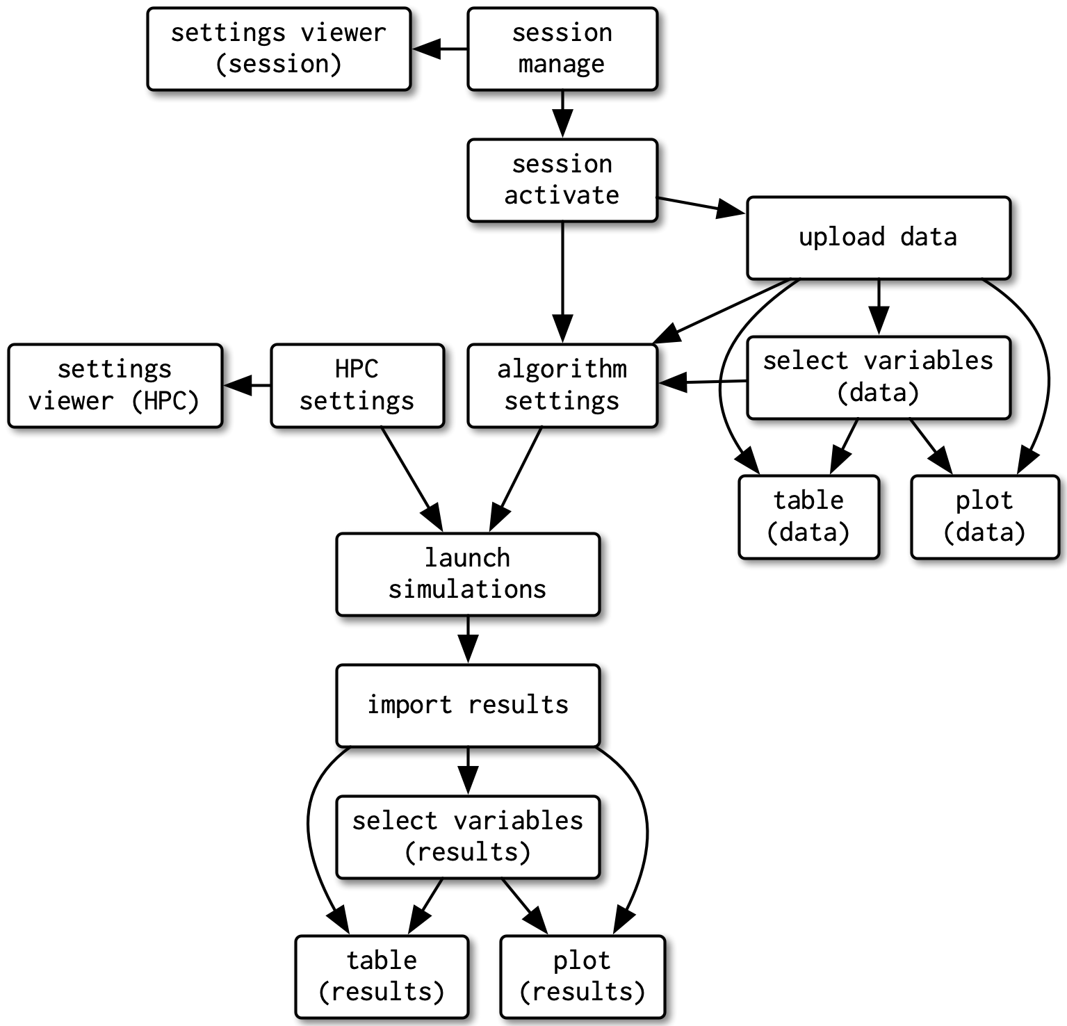
This app has many parts and pieces with complicated connectivity and dependencies.
Redesigning (“refactoring”) to use modules allowed Eric to clearly distinguish the separate parts of the app and their relationships with each other.
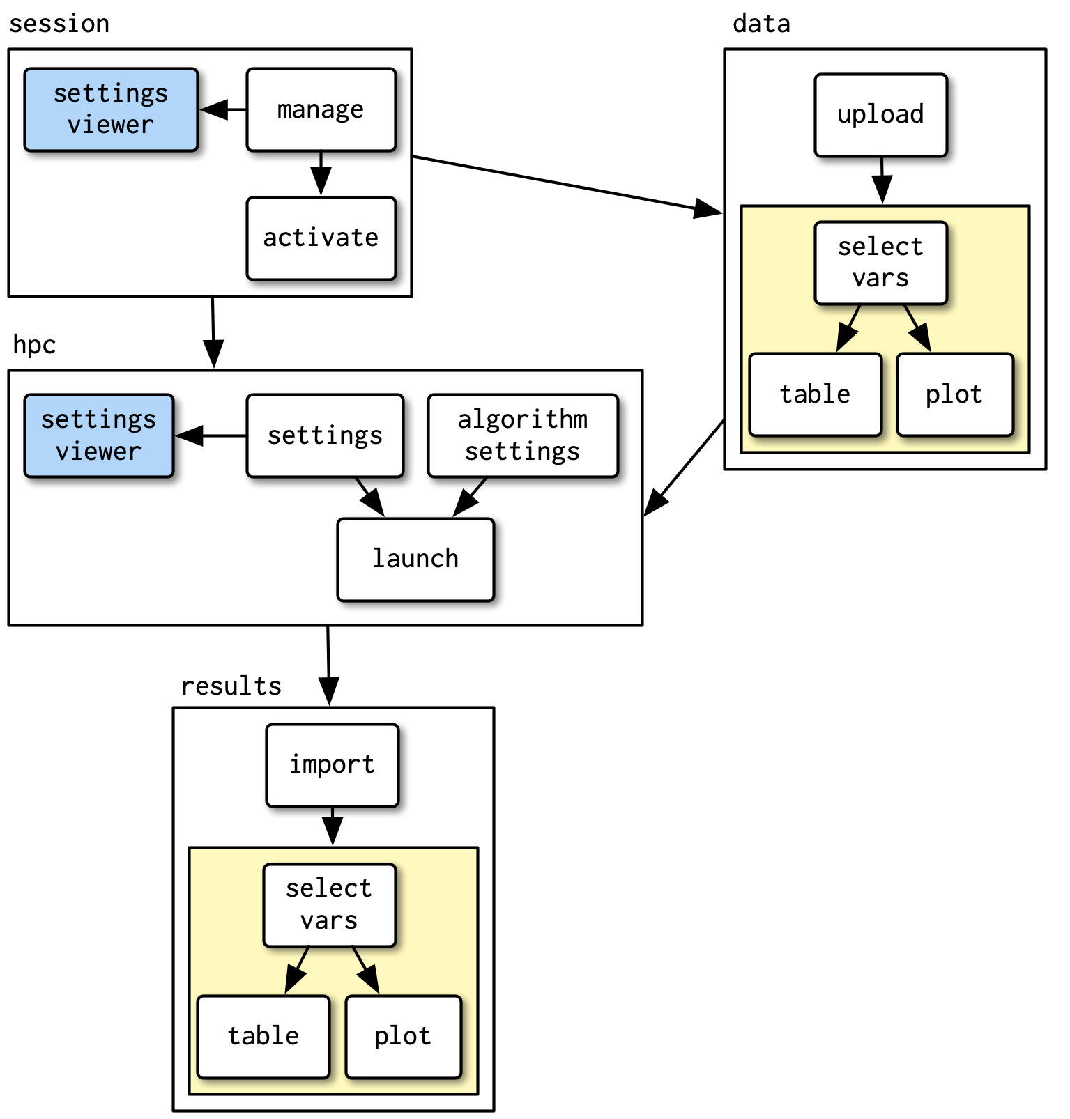
11.9.1.2 Implications of Using Modules
A module is a sealed box to other modules.
- All interactions are limited to those defined by the interface for the module.
- Other modules can’t access or change anything inside a different module not present in the interface
Each module has its own name (and namespace)so we can simplify naming across the app.
Each module is also reusable and can be called from other modules - see the yellow and blue examples
- Modules can access functions sourced from separate
fct*.Rfiles
Bottom Line: Modules extend the benefits of separation and reducing duplication to much greater level than functions alone.
11.9.2 Module Basics
- A module is very similar to a shiny app in that it has two pieces:
- The module UI function that generates the
uispecification. - The module server function that runs the code for the server.
- The module UI function that generates the
- These two functions have standard forms.
- They both take
idas the first argument and use it to namespace the module.
- However the packaging is different in important ways.
- They both take
To create a module, we need to extract code out of the the app UI and server and put it in to the module UI and server.
Let’s start with the UI section.
11.9.2.1 Creating a Module UI
This looks like normal UI code with a few important differences:
- It’s inside its own named function with
idas the first argument - The first line in the function body uses the
NS(id)function to create and save the namespace foridto variablens - All input and output IDs that appear in the function body get wrapped in a call to
ns().
- The example below shows inputId arguments being wrapped in
ns(), e.g.ns("file")). - If we happened to have a
plotOutputin our UI, we would also want to usens()when declaring itsoutputId.
- The results are wrapped in
tagList(), instead offluidPage(),pageWithSidebar(), etc..
- You only need to use
tagList()if you want to return a UI fragment with multiple UI objects; if you are just returning a div or a single input, you could skiptagList().
Here’s an example for a CSV file input module:
# Module UI function
csvFileUI <- function(id, label = "CSV file") {
  # `NS(id)` returns a namespace function, which we save as `ns` and will
  # invoke later.
  ns <- NS(id)

  tagList(
    fileInput(ns("file"), label),
    checkboxInput(ns("heading"), "Has heading"),
    selectInput(ns("quote"), "Quote", c(
      "None" = "",
      "Double quote" = "\"",
      "Single quote" = "'"
    ))
  )
}- Using
tagList()is flexible because it allows the caller of the module to choose the container. - Using
ns()may seem onerous but it frees you from having to make sure your IDs are unique across all other modules - the “secret sauce” to modules.
11.9.2.2 The Module Server
The server logic gets encapsulated in a single function we’ll call the module server function.
Module server functions should be named like their corresponding module UI functions, but with a “server” suffix instead of “Input/Output/UI”.
- We’ll call our server function
csvFileServer(). - Ensure this function calls
moduleServer()with the id, and a function that looks like a regular server function, i.e.,function(input, output, session)and enter the code insidemoduleServer()as an expression (inside{})
# Module server function
csvFileServer <- function(id, stringsAsFactors) {
  moduleServer(
    id,
## Below is the module function
    function(input, output, session) {
  # The selected file, if any
      userFile <- reactive({
    # If no file is selected, don't do anything
        validate(need(input$file, message = FALSE))
        input$file
      })

  # The user's data, parsed into a data frame
      dataframe <- reactive({
        read.csv(userFile()$datapath,
          header = input$heading,
          quote = input$quote,
          stringsAsFactors = stringsAsFactors
        )
      })

  # We can run observers in here if we want to
      observe({
        msg <- sprintf("File %s was uploaded", userFile()$name)
        cat(msg, "\n")
      })

  # Return the reactive that yields the data frame
      return(dataframe)
    }
  )
}
The two levels of functions are important as they help distinguish the argument to your module from the arguments to the server function.
- The
moduleServer()function invokes the module function in a special way that creates special input, output, and session objects that are aware of theid. - Don’t worry if the beginning looks complex; it’s basically boilerplate you can copy and paste for each new module you create.
- The outer function,
csvFileServer(), takesidas its first parameter.
You can define the function to take any number of additional parameters, including …, so whoever uses the module can customize what the module does.
- In this case, there’s one extra parameter,
stringsAsFactors, so the application using this module can decide whether or not to convert strings to factors when reading in the data.
The code inside the module function can use parameters from the outer function’s arguments.
You can have as many or as few additional parameters as you want, including
....Inside the module function, we can use
input$fileto refer to thens("file")component in the UI function.- If this example had outputs, we could similarly match up
ns("plot")withoutput$plot.
- If this example had outputs, we could similarly match up
The input, output, and session objects we’re provided with are special, in that they use the id to scope them to the specific namespace that matches up with our UI function.
- On the flip side, the input, output, and session cannot be used to access inputs/outputs outside of the namespace, nor can they directly access reactive expressions and reactive values from elsewhere in the application; the module is “isolated”.
The goal is not to prevent modules from interacting with their containing apps; The goal is to make these interactions explicit.
- If a module needs to use a reactive expression, the outer function should take the reactive expression as a parameter.
- If a module wants to return reactive expressions to the calling app, then return a list of reactive expressions from the function.
11.9.2.3 Namespacing Revisited
Key idea: the name (id) of each control in a module when its executing is now determined by two pieces:
- The first piece comes from the module user (the external calling module).
- The second piece comes from the module author (internal to your module namespace).
- This two-part specification means that you, the module author, don’t need to worry about clashing with other UI components created by the user (calling module).
- You have your own “space” of names, that you own, and can arrange to best meet your own needs.
11.9.2.4 Naming Conventions
This example uses a special naming scheme for all the components of the module.
- This is a recommended best practice
If we were to create a module to draw a histogram, we could call it the histogram module.
- This base name is then used in a variety of places:
R/histogram.Rholds all the code for the module.histogramUI()is the module UI. A module’s UI function should have a name with suffixInput,Output, orUI;- If you have modules primarily for input or output, call them
histogramInput()orhistogramOuput()instead of UI.
- If you have modules primarily for input or output, call them
histogramServer()is the module server.histogramApp()creates a complete app for interactive experimentation and more formal testing.
11.9.3 Using Modules in a Shiny App
Assuming the above csvFileUI and csvFileServer functions are loaded (more on that in a moment), this is how you’d use them in a Shiny app:
library(shiny)
# UI Section
ui <- fluidPage(
  sidebarLayout(
    sidebarPanel(
      csvFileUI("datafile", "User data (.csv format)") ### module call
    ),
    mainPanel(
      dataTableOutput("table")
    )
  )
)
# Server Section
server <- function(input, output, session) {
  datafile <- csvFileServer("datafile",
    stringsAsFactors = FALSE
  ) ### module call

  output$table <- renderDataTable({
    datafile()
  })
}

shinyApp(ui, server)
The UI function csvFileUI is called directly, using "datafile" as the id.
- In this case, we’re inserting the generated UI into the sidebar panel.
The module server function is called with csvFileServer(), with the id that we will use as the namespace;
- This must be exactly the same as the
idargument we passed tocsvFileUI. - The call to the module server function also is passed the parameter
stringsAsFactors = FALSE.
Like all Shiny modules, csvFileUI can be embedded in a single app more than once.
- Each call must be passed a unique
id, and each call must have a corresponding call tocsvFileServer()on the server side with that sameid.
11.9.3.1 Another Example
Let’s use a module to create linked scatter plots (selecting an area on one plot will highlight observations on both plots).
11.9.3.2 The module UI function.
We want two plots, plot1 and plot2, side-by-side with a common brush id of brush.
- The brush
idneeds to be wrapped inns(), just like the plotOutputids.
11.9.3.3 The Module Server Function
Besides the mandatory input, output, and session parameters, we need to know:
- the data frame to plot (
data), and - the column names for the
xandyfor each plot (leftandright).
To allow the data frame and columns to change in response to user actions, the data, left, and right must all be reactive expressions.
- These parameters are passed to
linkedScatterServer, and they can be used in the module function defined inside.
linkedScatterServer <- function(id, data, left, right) {
  moduleServer(
    id,
    function(input, output, session) {
  # boilerplate above

  # Yields the data frame with an additional column "selected_"
  # that indicates whether that observation is brushed
      dataWithSelection <- reactive({
        brushedPoints(data(), input$brush, allRows = TRUE)
      })

      output$plot1 <- renderPlot({
        scatterPlot(dataWithSelection(), left())
      })

      output$plot2 <- renderPlot({
        scatterPlot(dataWithSelection(), right())
      })

      return(dataWithSelection)
    }
  )
}- Notice the module function inside of
linkedScatterServer()returns thedataWithSelectionas reactive.- This means the caller of this module can make use of the brushed data as well, such as showing it in a table below the plots, for example.
For clarity and ease of testing, let’s put the plotting code in a standalone function called scatterPlot().
- The
scale_color_manualcall sets the colors of unselected vs. selected points, andguide = FALSEhides the legend.
11.9.3.4 Putting it all together
Run after running the previous three blocks to source each function.
library(shiny)

# UI Section
ui <- fixedPage(
  h2("Module Example"),
  linkedScatterUI("scatters"),
  textOutput("summary")
)

# Server Section
server <- function(input, output, session) {
  df <- linkedScatterServer("scatters", reactive(mpg),
    left = reactive(c("cty", "hwy")),
    right = reactive(c("drv", "hwy"))
  )

  output$summary <- renderText({
    sprintf(
      "%d observation(s) selected",
      nrow(dplyr::filter(df(), selected_))
    )
  })
}

shinyApp(ui, server)
11.9.4 Nesting Modules
Since they are isolated functions, Modules can use other modules.
- When doing so, when the outer module’s UI function calls the inner module’s UI function, ensure the
idis wrapped inns().
In the following example, when outerUI calls innerUI, notice the id argument is ns("inner1").
As for the module server functions, just ensure the call to the inner module happens inside the outer module’s server function.
- There’s generally no need to use
ns().
11.9.5 Organizing and Accessing your Modules
The previous examples of using a module assume that the module’s UI and server functions are defined and available.
- But logistically, where should these functions actually be defined, and how should they be loaded into R?
There are several options.
- Inline code.
- Most simply, you can put the UI and server function code directly in your app.
- If you’re using a single app.R file, just include the code for your module functions right in that file, before the app’s UI and server logic.
- If you’re using a ui.R/server.R style file layout, add a
global.Rfile to your app directory (if you don’t already have one) and put the UI and server functions there. - The
global.Rfile will be loaded before eitherui.Rorserver.R. - However, if you have many modules to define, or modules that contain a lot of code, this may result in a bloated
global.R/app.Rfile so consider other options.
- In an R script in the
Rsubdirectory.- You can create a separate R script (.R file) for the module in the
Rsubdirectory of your application. - It will automatically be sourced (as of Shiny 1.5.0) when the application is loaded.
- This is the recommended method for modules that won’t be reused across applications.
- You can create a separate R script (.R file) for the module in the
- In an R script elsewhere in the app directory.
- You can create a separate R script (.R file) for the module, either directly in the app directory or in a subdirectory.
- Then call
source("path-to-module.R")(from app.R or from global.R (if using ui.R/server.R). This will add your module functions to the global environment. - In versions of Shiny prior to 1.5.0, this was the recommended method, but with 1.5.0 and later, it’s recommend to use the previous method, where the standalone R script is in the R/ subdirectory.
- Create an R package.
- For modules you intend to reuse in other applications, consider building an R package.
- Your R package needs to export and document your module’s UI and server functions.
- You can include more than one module in a package, if you like.