Computer-based Text Mining has been around since the 1950s with automated translations, or the 1940s if you want to consider computer-based code-breaking Trying to Break Codes.
In addition to text mining or analysis, NLP has multiple areas of research and application.
Machine Translation: translation without any human intervention.
Speech Recognition: Alexa, Hey Google, Siri, … understanding your questions.
Sentiment Analysis: also known as opinion mining or emotion AI.
Question Answering: Alexa, Hey Google, Siri, … answering your questions so you can understand.
Automatic Summarization: Reducing large volumes to meta-data or sensible summaries.
Chat bots: Combinations of 2 and 4 with short-term memory and context for specific domains.
Market Intelligence: Automated analysis of your searches, posts, tweets, ….
Text Classification: Automatically analyze text and then assign a set of pre-defined tags or categories based on its content e.g., organizing and determining relevance of reference material
Character Recognition.
Spelling and Grammar Checking.
Text Analysis/Natural Language processing is a basic technology for generative AIs What is generative AI?.
15.3 Organizing Text for Analysis and Tidy Text Format
There are multiple ways to organize text for analysis:
strings: character data in atomic vectors or lists (data frames)
corpus: a library of documents structured as strings with associated metadata, e.g., the source book or document
Document-Term Matrix (DTM): a matrix with a row for each document and a column for every unique term or word across every document (i.e., across all rows).
The entries are generally counts or tf-idf (term frequency - inverse document freq) scores for the column’s word in the row’s document.
With multiple rows, there are a lot of 0s, so usually stored as a sparse matrix.
The Term-Document Matrix (TDM) is the transpose of the DTM.
We will focus on organizing bodies of text into Tidy Text Format (TTF).
Tidy Text Format requires organizing text into a tibble/data frame with the goal of speeding analysis by allowing use of familiar tidyverse constructs.
In a TTF tibble, the text is organized so as to have one token per row.
A token is a meaningful unit of text where you decide what is meaningful to your analysis.
A token can be a word, an n-gram (multiple words), a sentence, a paragraph, or even larger sets up to whole chapters or books..
The simplest approach is analyzing single words or n-grams without any sense of syntax or order connecting them to each other.
This is often called a “Bag of Words” as each token is treated independently of the other tokens in the document; only the counts or tf-idfs matter.
More sophisticated methods are now using neural word embeddings where the words are encoded into vectors that attempt to capture (through training) the context from other words in the document (usually based on physical or semantic distance.
Before diving into specific tools and functions, it is helpful to understand a general workflow for preparing text for analysis.
These steps provide a consistent structure you can adapt depending on your data source and analytical goals.
For most introductory text analyses, a reasonable workflow uses multiple steps to prepare (pre-process) text data for analysis and minimize “invisible” errors that can arise from different representations of the same text.
Preserve the raw text unchanged (similar to preserving raw data of any sort)
Always keep an original copy of the text exactly as it was collected. This ensures you can return to the source data if needed and helps avoid introducing irreversible errors during cleaning.
Create a cleaned copy for analysis.
Perform all transformations on a separate version of the text. This allows you to experiment with different cleaning strategies without affecting the original data.
Standardize Unicode representations.
Text data may contain multiple representations of the same characters (e.g., different types of quotation marks or accented letters).
Standardizing Unicode ensures visually identical text is converted to a single internal representation so it is treated consistently by your code.
While Unicode standardization ensures equivalent characters are represented consistently,
normalization (Step 4) goes a step further by simplifying text to reduce variation that may interfere with analysis.
NoteUnicode
Unicode is a global standard for representing text in computers that assigns a unique code to each character across languages and symbol systems.
For example, the letter “é” can be stored as a single character or as a combination of “e” plus an accent mark.
Single pre-composed character (NFC form):
Code point: U+00E9
Name: LATIN SMALL LETTER E WITH ACUTE
This is a single character.
Decomposed form (NFD form)
Code points:
U+0065 → LATIN SMALL LETTER E
U+0301 → COMBINING ACUTE ACCENT
This is two characters: “e” + a combining accent applied to it.
Visually, these look identical:
é  (U+00E9)
é (U+0065 + U+0301)
But computationally, they are different sequences of characters.
These “invisible” differences can cause problems in code-based text analysis. Examples include:
string matching can fail (“é” != “é”) when one is NFC and one is NFD.
tokenization can split the same apparent word into multiple forms
joins and comparisons may silently break
That is why standardization is important as it converts text to a consistent internal representation before further processing to minimize “invisible” errors.
Standardization functions (such as in {stringi}) use rules established in the Unicode standard to choose among the valid representations in a deterministic, repeatable manner.
For example, NFC form is often preferred for text analysis as it treats accented characters as single units which aligns better with tokenization and word-level analysis.
A typical step would be text <- stringi::stri_trans_nfc(text) to convert all text to NFC form.
Standardizing Unicode early in the workflow helps ensure equivalent text is treated consistently throughout the analysis.
Simplify the Text (as appropriate) by Normalizing punctuation and transliterating accented Latin characters.
After standardizing Unicode representations, the text is internally consistent but may still contain stylistic or semantically equivalent variations (e.g., dash types, quotation styles, accented characters) that can affect analysis.
Normalization is a deliberate simplification step that converts these variations into a consistent form to improve tokenization, matching, and aggregation.
Examples include:
converting different dash types (e.g., em dash, en dash) to a standard hyphen
standardizing quotation marks or removing punctuation where appropriate
optionally transliterating accented characters, e.g., “é” → “e”, may further reduce variation across text sources.
Unlike Unicode standardization, normalization may change the text, so it should be applied based on the goals of the analysis.
Normalization improves consistency, but transliteration is a lossy transformation and may remove meaningful distinctions.
Step 4 (normalization) simplifies text for analysis but may change the text in ways that affect meaning or interpretation.
NoteTransliteration and Meaning
Transliteration converts characters from one form to another, often mapping accented or non-ASCII characters to simpler ASCII equivalents.
Example: “café” → “cafe”
Example: “naïve” → “naive”
This can be helpful for:
simplifying text for matching and counting
reducing duplicate tokens caused by minor spelling variations
working with systems that expect ASCII text
However, transliteration can also affect meaning or interpretation:
Different words may collapse into the same form
Proper names and words borrowed from other languages (“loanwords”) may lose important distinctions
In some languages, diacritics distinguish entirely different words
Examples include:
“résumé” -> “resume”
résumé = a document summarizing experience
resume = to continue after a pause
“exposé” -> “expose”
exposé = a report revealing something (often wrongdoing)
expose = the verb “to reveal” or “to uncover”
As a result, transliteration should be used intentionally, based on the goals of the analysis.
It is often appropriate for exploratory analysis and frequency-based methods
It may be inappropriate when exact spelling, linguistic nuance, or semantic precision matters
TipExample: Standardization and Normalization with {stringi}
The {stringi} package provides functions to standardize Unicode and normalize text in a consistent and reproducible way.
library(stringi)text_raw <-c("café — “quoted text”", "caché isn’t the same as cache")# Step 3: Standardize Unicode (NFC)text_nfc <- stringi::stri_trans_nfc(text_raw)# Step 4: Normalize punctuation and optionally transliteratetext_clean <- text_nfc |> stringi::stri_replace_all_fixed("—", "-") |># em dash → hyphen stringi::stri_replace_all_fixed("“", "\"") |># left quote → " stringi::stri_replace_all_fixed("”", "\"") |># right quote → " stringi::stri_replace_all_fixed("’", "'") |># curly apostrophe → ' stringi::stri_trans_general("Latin-ASCII") # transliterationtext_raw
[1] "café — “quoted text”" "caché isn’t the same as cache"
text_clean
[1] "cafe - \"quoted text\"" "cache isn't the same as cache"
Tokenize the text into the unit needed for the analysis.
Tokenizing breaks the text into meaningful tokens (units) such as words, n-grams, sentences, or paragraphs.
The choice of token depends on the goal of the analysis, e.g., word frequency vs. sentiment by sentence.
Remove or customize stop words when appropriate.
Common words (e.g., “the”, “and”) are often removed to focus on meaningful content.
However, in some analyses (such as sentiment or phrase detection), these words may carry important information and should be retained or customized.
Document each cleaning choice because preprocessing decisions affect results.
Every cleaning step changes the data. Keeping track of these decisions ensures reproducibility and helps explain differences in results across analyses.
In the following sections, we will consider each of these steps using {tidytext}, {stringr}, and {stringi} as we move from raw text to structured, analyzable data.
15.5 The {tidytext} package
The {tidytext} package contains many functions to support text mining for word processing and sentiment analysis.
It is designed to work well with other tidyverse packages such as {dplyr} and {ggplot2}.
Use the console to install the package and then load {tidyverse} and {tidytext}.
text <-c("If You Forget Me","by Pablo Neruda","I want you to know","one thing.","You know how this is:","if I look","at the crystal moon, at the red branch","of the slow autumn at my window,","if I touch","near the fire","the impalpable ash","or the wrinkled body of the log,","everything carries me to you,","as if everything that exists,","aromas, light, metals,","were little boats","that sail","toward those isles of yours that wait for me.")text
 [1] "If You Forget Me"
 [2] "by Pablo Neruda"
 [3] "I want you to know"
 [4] "one thing."
 [5] "You know how this is:"
 [6] "if I look"
 [7] "at the crystal moon, at the red branch"
 [8] "of the slow autumn at my window,"
 [9] "if I touch"
[10] "near the fire"
[11] "the impalpable ash"
[12] "or the wrinkled body of the log,"
[13] "everything carries me to you,"
[14] "as if everything that exists,"
[15] "aromas, light, metals,"
[16] "were little boats"
[17] "that sail"
[18] "toward those isles of yours that wait for me."
Let’s get some basic info about our text.
Check the length of the vector.
Use map() to check the number of characters in each element.
Use map_dbl() to count the number of words in each element and total number of words.
You get a character variable of length 18 with 80 words.
Each element has different numbers of words and letters.
This is not a tibble so it can’t be tidy text format with one token per row.
We’ll go through a number of steps to gradually transform the text vector to tidy text format and then clean it so we can analyze it.
Note: In this example, we skip Unicode standardization and normalization because the text is already clean and does not contain accented characters or inconsistent punctuation.
In real-world text data (e.g., OCR text, web scraping, larger or historical works or multilingual sources), these preprocessing steps are often necessary before tokenization.
15.5.1.1 Convert the text Vector into a Tibble
Convert text into a tibble with two columns:
Add a column line with the “line number” from the poem for each row based on the position in the vector.
Add a column text with the each element of the vector in its own row.
Adding a column of indices for each token is a common technique to track the original structure.
# A tibble: 10 × 2
    line text
   <int> <chr>
 1     1 If You Forget Me
 2     2 by Pablo Neruda
 3     3 I want you to know
 4     4 one thing.
 5     5 You know how this is:
 6     6 if I look
 7     7 at the crystal moon, at the red branch
 8     8 of the slow autumn at my window,
 9     9 if I touch
10    10 near the fire
15.5.1.2 Convert the Tibble into Tidy Text Format with unnest_tokens()
The function unnest_tokens(text_df) converts a column of text from a data frame into tidy text format.
Look at help for unnest_tokens(), not the older unnest_tokens_().
The first argument, tbl, is the input tibble so piping works.
The order might be un-intuitive as output is next, followed by the input column.
Like unnesting list columns, unnest_tokens() splits each element (row) in the column into multiple rows with a single token.
The value of the token is based on the value of the argument token = which recognizes multiple options
“words” (default), “characters”, “character_shingles”, “ngrams”, “skip_ngrams”, “sentences”, “lines”, “paragraphs”, “regex”, “tweets” (tokenization by word that preserves usernames, hashtags, and URLS), and “ptb” (Penn Treebank).
# A tibble: 10 × 2
    line word
   <int> <chr>
 1     1 if
 2     1 you
 3     1 forget
 4     1 me
 5     2 by
 6     2 pablo
 7     2 neruda
 8     3 i
 9     3 want
10     3 you
# or use the pipetext_df |>unnest_tokens(output = word,input = text ) |>head(10)
# A tibble: 10 × 2
    line word
   <int> <chr>
 1     1 if
 2     1 you
 3     1 forget
 4     1 me
 5     2 by
 6     2 pablo
 7     2 neruda
 8     3 i
 9     3 want
10     3 you
This converts the data frame to 80 rows with a one-word token in each row.
Punctuation has been stripped.
By default, unnest_tokens() converts the tokens to lowercase.
Use the argument to_lower = FALSE to retain case.
15.5.2 Remove Stop Words with an anti_join() on stop_words
We can see a lot of common words in the text such as “I”, “the”, “and”, “or”, ….
These are called stop words: extremely common words not useful for some types of text analysis.
Use data() to load the {tidytext} package’s built-in data frame called stop_words.
stop_words draws on three different lexicons to identify 1,149 stop words (see help).
Use anti_join() to remove the stop words (a filtering join that removes all rows from x where there are matching values in y).
Save to a new tibble.
How many rows are there now?
data(stop_words)text_df |>unnest_tokens(word, text) |>anti_join(stop_words, by ="word") |>## get rid of uninteresting wordscount(word, sort =TRUE) ->## count of each word lefttext_word_counttext_word_count
# A tibble: 26 × 2
   word        n
   <chr>   <int>
 1 aromas      1
 2 ash         1
 3 autumn      1
 4 boats       1
 5 body        1
 6 branch      1
 7 carries     1
 8 crystal     1
 9 exists      1
10 fire        1
# ℹ 16 more rows
nrow(text_word_count) ## note: only 26 rows instead of 80
[1] 26
These are the basic steps to get your text ready for analysis:
Convert text to a tibble, if not already in one, with a column for the text and an index column with row number or other location indicators.
Convert the tibble to Tidy Text format using unnest_tokens() with the appropriate arguments.
Remove stop words if appropriate (sometimes we need to keep them as we will see later).
Save to a new tibble.
15.6 Tidytext Example 2: Jane Austen’s Books and the {janeaustenr} Package
Let’s look at a larger set of text, all six major novels written by Jane Austen in the early 19th century.
The {janeaustenr} package has this text already in a data frame based on the free content in the Project Gutenberg Library.
Note: The text from the {janeaustenr} package is curated and relatively clean, so we do not need to perform Unicode standardization or normalization in this example.
In practice, these preprocessing steps are important when working with less structured or multi-source text data.
Use the console to install the package and then use library() to load and attach it.
library(janeaustenr)
15.6.1 Get the Data for the Corpus of Six Books and Add Metadata
Use the function austen_books() to access the data frame of the six books.
The data frame has two columns:
text contains the text of the novels divided into elements of up to about 70 characters each.
book contains the titles of the novels as a factor, with the levels in order of publication.
We want to track the chapters in the books.
Let’s use REGEX to see how the different books indicate their chapters.
austen_books() |>head(20)
# A tibble: 20 × 2
   text                                                                    book
   <chr>                                                                   <fct>
 1 "SENSE AND SENSIBILITY"                                                 Sens…
 2 ""                                                                      Sens…
 3 "by Jane Austen"                                                        Sens…
 4 ""                                                                      Sens…
 5 "(1811)"                                                                Sens…
 6 ""                                                                      Sens…
 7 ""                                                                      Sens…
 8 ""                                                                      Sens…
 9 ""                                                                      Sens…
10 "CHAPTER 1"                                                             Sens…
11 ""                                                                      Sens…
12 ""                                                                      Sens…
13 "The family of Dashwood had long been settled in Sussex.  Their estate" Sens…
14 "was large, and their residence was at Norland Park, in the centre of"  Sens…
15 "their property, where, for many generations, they had lived in so"     Sens…
16 "respectable a manner as to engage the general good opinion of their"   Sens…
17 "surrounding acquaintance.  The late owner of this estate was a single" Sens…
18 "man, who lived to a very advanced age, and who for many years of his"  Sens…
19 "life, had a constant companion and housekeeper in his sister.  But he… Sens…
20 "death, which happened ten years before his own, produced a great"      Sens…
Chapters start on their own line it appears.
austen_books() |>filter(str_detect(text, "(?i)^chapter")) |># Case insensitiveslice_sample(n =10)
# A tibble: 10 × 2
   text       book
   <chr>      <fct>
 1 CHAPTER IV Emma
 2 CHAPTER 30 Sense & Sensibility
 3 CHAPTER 36 Sense & Sensibility
 4 CHAPTER XV Emma
 5 CHAPTER 4  Northanger Abbey
 6 Chapter 17 Pride & Prejudice
 7 Chapter 44 Pride & Prejudice
 8 CHAPTER 40 Sense & Sensibility
 9 CHAPTER 3  Sense & Sensibility
10 Chapter 21 Pride & Prejudice
Chapters start with the word chapter in both upper and sentence case followed by a space then the chapter number in either Arabic or Roman numerals.
Let’s add some metadata to keep track of things when we convert to tidy text format.
Group by book.
Add an index column with a row number for the rows from each book (they are grouped).
Add an index column with the number of the chapter.
Use stringr::regex() with argument ignore_case = TRUE.
regex() is a {stringr} modifier function with options for how to modify the regex pattern.
We can now see the book, chapter, and line number for each of the 73,422 text elements with almost 730K (non-unique) individual words.
15.6.2 Convert to Tidy Text Format, Clean, and Sort the Counts
Unnest the text with the tokens being each word.
Clean the words to remove any formatting characters.
Project Gutenberg uses pairs of formatting characters, before and after a word, to denote bold or italics e.g., “_myword_” means myword.
We want to extract just the words without any formatting symbols.
Remove stop words.
Save to a new tibble.
Look at the number of rows and the counts for each unique word.
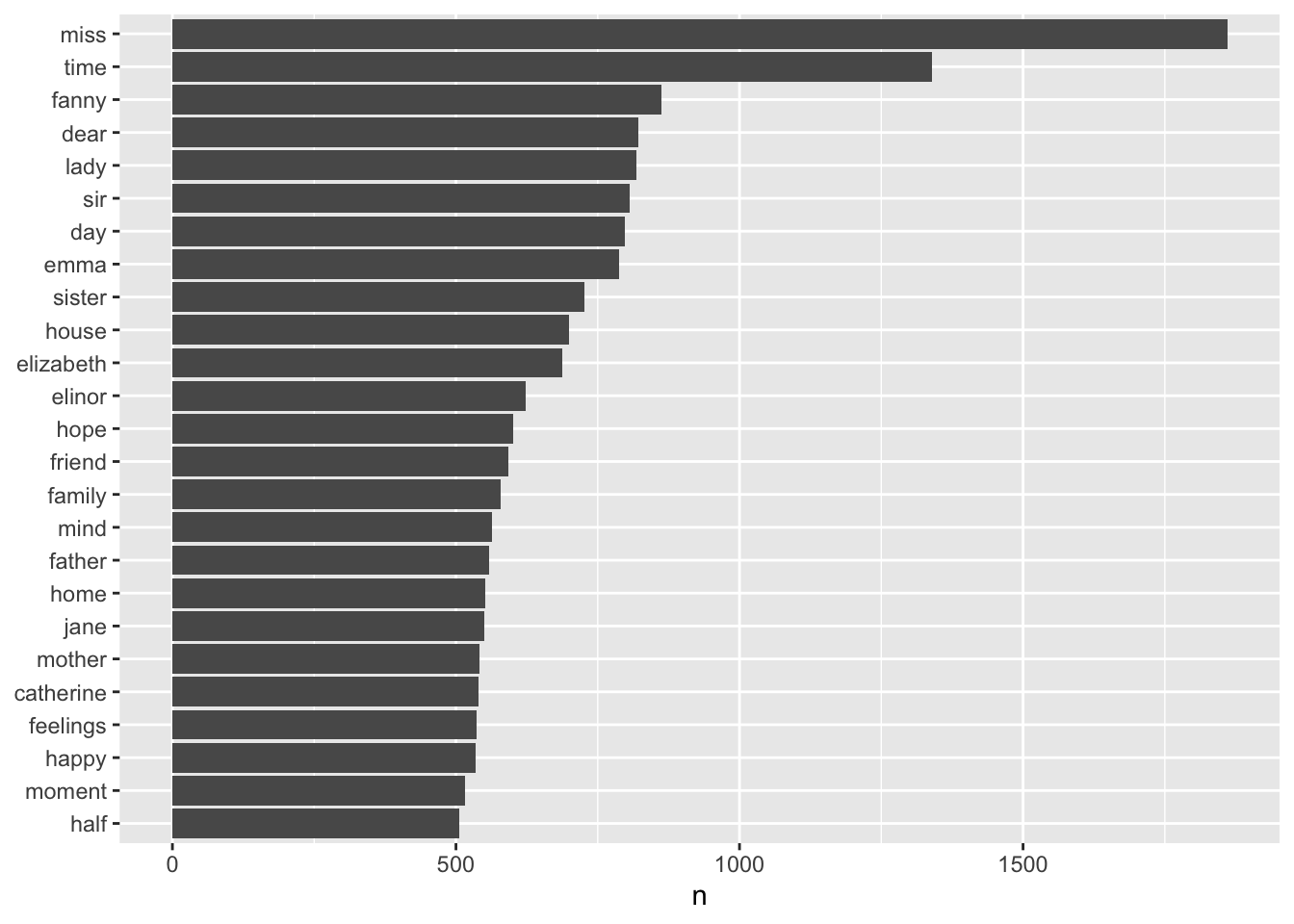
orig_books |>unnest_tokens(word, text) |>## nrow() #725,055## use str_extract to get just the words inside any format encodingmutate(word =str_extract(word, "[a-z']+")) |>anti_join(stop_words, by ="word") ->## filter out words in stop_wordstidy_booksnrow(tidy_books)
# A tibble: 13,464 × 2
   word       n
   <chr>  <int>
 1 miss    1860
 2 time    1339
 3 fanny    862
 4 dear     822
 5 lady     819
 6 sir      807
 7 day      797
 8 emma     787
 9 sister   727
10 house    699
# ℹ 13,454 more rows
There are 216,385 instances of 13,464 unique (non-stop word) words across the six books.
The data are now in tidy text format and ready to analyze!
15.6.3 Plot the Most Common Words
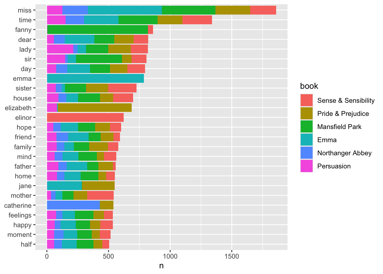
Let’s plot the “most common” words (defined for now as more than 500 occurrences) in descending order by count.
# A tibble: 6 × 3
# Groups:   book [6]
  word     book                count
  <chr>    <chr>               <int>
1 elinor   Sense & Sensibility   623
2 crawford Mansfield Park        493
3 weston   Emma                  389
4 darcy    Pride & Prejudice     374
5 elliot   Persuasion            254
6 tilney   Northanger Abbey      196
Show code
# note Emma occurs once in Persuasion
How would you change your code if you did not know how many books there were or there were many books?
Show code
## Without knowing how many books or titlestidy_books |>group_by(book) |>count(word, sort =TRUE) |>ungroup() |>pivot_wider(names_from = book, values_from = n) |>mutate(across(where(is.numeric), is.na, .names ="na_{ .col}")) |>rowwise() |>mutate(tot_books =sum(c_across(starts_with("na")))) |>ungroup() |>## have to ungroup after rowwisefilter(tot_books ==max(tot_books)) |>select(!(starts_with("na_") |starts_with("tot"))) |>pivot_longer(-word,names_to ="book", values_to ="count",values_drop_na =TRUE ) |>group_by(book) |>filter(count ==max(count)) |>arrange(desc(count))
# A tibble: 6 × 3
# Groups:   book [6]
  word     book                count
  <chr>    <chr>               <int>
1 elinor   Sense & Sensibility   623
2 crawford Mansfield Park        493
3 weston   Emma                  389
4 darcy    Pride & Prejudice     374
5 elliot   Persuasion            254
6 tilney   Northanger Abbey      196
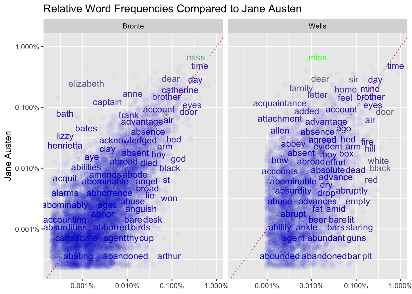
15.7 Compare Frequencies across Authors
Let’s compare Jane Austen to two other writers:
H.G. Wells a science fiction writer (The Island of Doctor Moreau, The War of the Worlds, The Time Machine, and The Invisible Man).
The Bronte Sisters (Jane Eyre, Wuthering Heights, Agnes Grey, The Tenant of Wildfell Hall and Villette) who are from Jane Austen’s era and genre.
Let’s compare Austen to the others based on how often each used specific words (non-stop words).
Note: Unlike the {janeaustenr} package, which provides curated text, data downloaded from Project Gutenberg may contain inconsistencies in punctuation, encoding, and formatting.
These differences can affect tokenization and especially matching with sentiment lexicons, so we will include a basic standardization and normalization step before analysis.
As a strategy, consider the following steps:
Identify several books from the two new authors so we have a reasonable data set.
Use Project Gutenberg and the {gutenbergr} package.
Download and clean each author’s books, then transform them into tidy text format.
Standardize Unicode representations
Normalize punctuation and, when appropriate, transliterate accented characters
Remove formatting artifacts and stop words
Remove formatting and stop words.
Add author to each tibble and combine into one tibble.
For each author get the relative frequencies of word usage.
Now we have to consider how to get the data into a form that is easy for comparison.
Consider using scatter plots to comparing Austen against Bronte and then Austen against Wells.
That suggests reshaping the data frame so that Austen’s frequencies are in one column and Bronte and Wells are in a second column, say author, so we can facet on author.
To facilitate the comparison, we can add a geom_abline() where the frequencies are equal.
To complete our strategy:
Reshape the Tibble.
Pivot wider to break out each author into three columns.
Pivot longer to combine Bronte and Wells into one author column.
Plot the relative frequencies for Austen versus the other author
Use a scatter plot.
Add a default geom_abline().
Facet on author.
Interpret the plots.
Use cor.test() to test the correlations.
15.7.1 Identify works for each new author
15.7.1.1 Project Gutenberg and the {gutenbergr} package
The {gutenbergr} package includes metadata for 70K Project Gutenberg works, so they can be searched and retrieved.
These are works in the public domain (published over 95 years ago) that have been digitized and uploaded by volunteers.
Use the console to install the package if necessary and load the library in your file.
You will need to use devtools::install_github("ropensci/gutenbergr").
library(gutenbergr)
15.7.1.2 Find the gutenberg_ID for each work
Example: Frankenstein has gutenberg_ID = 84, so use gutenberg_download(84).
To find a work’s gutenberg_ID, use function gutenberg_works().
You can search on the “exact title” (as used in Project Gutenberg) or,
Look for the author in the author metadata gutenberg_authors data frame and then use the gutenberg_authors_id to find the work IDs for the author in gutenberg_works().
gutenberg_works(gutenberg_author_id ==30) |>arrange(title) |>mutate(stitle =str_trunc(title, 40)) |>## there are some very long titles.select(stitle, gutenberg_id) |>filter(str_detect(stitle, "Moreau")) ## if there are lots of titles
# A tibble: 2 × 2
  stitle                      gutenberg_id
  <chr>                              <int>
1 The island of Doctor Moreau          159
2 The island of Dr. Moreau           28840
15.7.2 Download and Preprocess the texts for Wells and Bronte into TTF
Use gutenberg_download() to download one or more works from Project Gutenberg.
Wells’ IDs are: (35, 36, 159, 5230).
Bronte’s IDs are: (767, 768, 969, 1260, 9182).
15.7.2.1 Standardizing and Normalizing Text
Because these texts come from Project Gutenberg, it is a good idea to standardize Unicode and normalize punctuation before tokenization.
This helps improve consistency in token counts and later matching with stop words and sentiment lexicons.
Let’s create a helper function for cleaning the text that we can apply to each author’s works before tokenization.
{stringi} is used here instead of {stringr} because it provides full support for Unicode normalization and transliteration (via ICU), which are not available in {stringr}.
{stringi} comes with numerous functions related to data cleansing, information extraction, and natural language processing in multiple languages, making it a powerful tool for text preprocessing.
The following example uses a series of {stringi} functions to standardize Unicode, normalize punctuation, and transliterate accented characters in a single pipeline.
It uses the “_fixed” versions of {stringi} functions.
Each step is explained with comments.
clean_text <-function(x) { x |> stringi::stri_trans_nfc() |># Standardize Unicode to NFC form# Ensures characters like "é" have a single consistent internal representation stringi::stri_replace_all_fixed("’", "'") |># Replace right curly apostrophe with standard ASCII apostrophe# Uses fixed replacement for speed and exact matching (no regex needed) stringi::stri_replace_all_fixed("‘", "'") |># Replace left curly apostrophe with ASCII apostrophe# Helps ensure consistency for contractions and possessives stringi::stri_replace_all_fixed("“", "\"") |># Replace left curly double quote with standard double quote stringi::stri_replace_all_fixed("”", "\"") |># Replace right curly double quote with standard double quote# Standardizing quotes helps avoid tokenization inconsistencies stringi::stri_replace_all_fixed("—", "-") |># Replace em dash with a standard hyphen# Different dash types are visually similar but treated differently in text processing stringi::stri_replace_all_fixed("–", "-") |># Replace en dash with a standard hyphen# Normalizing dash variants improves consistency in tokenization stringi::stri_trans_general("Latin-ASCII")# Transliterate accented Latin characters to ASCII equivalents (e.g., "café" → "cafe")# Useful for matching and aggregation, but is a lossy transformation# {stringi} provides ICU-based transliteration; {stringr} does not support this}
This uses the “_regex” version of {stringi} functions without comments.
When replacing text using {stringi}, there are two common approaches depending on how you want to match patterns:
stri_replace_all_fixed()
Treats the pattern as literal text
Replaces exact matches only (no special interpretation)
Faster and simpler
stri_replace_all_regex()
Treats the pattern as a regular expression (regex)
Allows flexible matching using patterns (e.g., multiple characters, wildcards)
More powerful, but slightly more complex
Examples
# Fixed: replace a specific characterstringi::stri_replace_all_fixed("don’t", "’", "'")# Regex: replace multiple variants in one stepstringi::stri_replace_all_regex("don’t", "[‘’]", "'")
Use fixed matching when:
replacing known characters (e.g., curly quotes, dashes)
you want simple, readable, and fast code
you are okay with writing separate lines for each replacement
Use regex matching when:
handling multiple variations at once
matching patterns (e.g., all punctuation, repeated spaces) e.g., for only replacing specific examples while leaving others in the original representation.
want more compact code with fewer lines.
Rule of thumb: use fixed matching by default, and switch to regex only when you need pattern flexibility.
Fixed matching is usually easier to understand; regex is more powerful but requires more care.
TipDebugging Unicode Characters
If text looks identical but does not match in your code, inspect the Unicode code points.
This can often happen when copying and pasting text from other applications, e.g., MSWord, or when combining text from different authors or sources.
As an example, to compare three visually similar dash characters, we can inspect their Unicode code points:
stringi::stri_enc_toutf32("—–-")
[[1]]
[1] 8212 8211   45
# or for formatted outputdata.frame(char = stringi::stri_split_boundaries("—–-", type ="character")[[1]],code =paste0("U+", toupper(format(as.hexmode(stringi::stri_enc_toutf32("—–-")[[1]])))))
  char   code
1    — U+2014
2    – U+2013
3    - U+002D
This reveals the underlying code points (e.g., U+2014 vs U+2013), which may differ even when characters look the same.
There are several ways to enter these characters in code, but the most precise and reproducible method is to use their Unicode code points.
text <-"This is an em dash: \u2014 and this is an en dash: \u2013"stringi::stri_replace_all_regex(text, "\\u2014", "-") # em dash
[1] "This is an em dash: - and this is an en dash: –"
[1] "This is an em dash: - and this is an en dash: -"
The syntax \\uXXXX represents a Unicode code point in regex patterns.
Tip: Using Unicode code points (e.g., \\u2014) avoids errors that can occur when copying visually similar characters.
15.7.2.2 Formatting Characters in Project Gutenberg and Other Sources
Text from Project Gutenberg and other open-source repositories often includes formatting artifacts that are not part of the actual content.
These may include:
underscores used to indicate emphasis (e.g., _word_)
asterisks or other markers for formatting
punctuation attached to words (e.g., word,, word.)
chapter headings, headers, and other structural text
These characters can interfere with tokenization and word matching by:
creating inconsistent tokens
preventing matches with stop words or sentiment lexicons
After standardizing Unicode, normalizing punctuation, and tokenizing the text, we can further clean individual tokens using a regular expression:
mutate(word =str_extract(word, "[a-z']+"))
[a-z’]+ keeps:
lowercase letters
apostrophes (useful for contractions like “don’t”)
This step removes:
other punctuation
formatting symbols
other non-letter characters
Note: This approach is designed for English text and is a simplification step. It may remove some information (e.g., numbers or special symbols) and should be adjusted based on the goals of the analysis.
If you want to preserve non-English characters, and did not transliterate, you can use \\p{L} use instead of [:alpha:] in regular expressions.
[:alpha:] matches alphabetic characters in the ASCII range, which generally corresponds to standard English letters (a–z, A–Z).
\\p{L} is a Unicode character class that matches any letter from any language, including:
accented characters (e.g., é, ñ, ü)
ligatures (e.g., æ, œ)
letters from non-English alphabets
For example:
"[a-z']+" → matches only lowercase English letters and apostrophes
"[\\p{L}']+" → matches all Unicode letters, including accented and non-English characters
In these notes, we use [a-z']+ (or [:alpha:]) because the text has been normalized to ASCII for compatibility with sentiment lexicons.
In more general text analysis, especially with multilingual data or when preserving accents, you may prefer \\p{L} to retain all valid letter characters and document your choices appropriately.
This step ensures tokens are consistent before counting or joining with other data (e.g., stop words or sentiment lexicons).
15.7.2.3 Complete Download and Preprocessing Steps
Now we are ready to execute several steps to get and pre-process the text for analysis.
Download the text for each author (as a tibble),
Standardize and normalize the text isimg the helper function clean_text().
Tokenize the text,
Remove formatting characters,
Remove NA values,
Remove Stop words,
Save in tibble with a name.
The text will be in tidy text format with one word per row and a column for the author.
# A tibble: 11,627 × 2
   word       n
   <chr>  <int>
 1 time     461
 2 people   302
 3 door     260
 4 heard    249
 5 black    232
 6 stood    229
 7 white    224
 8 hand     218
 9 kemp     213
10 eyes     210
# ℹ 11,617 more rows
tidy_bronte |>count(word, sort =TRUE)
# A tibble: 22,489 × 2
   word       n
   <chr>  <int>
 1 time    1066
 2 miss     856
 3 day      827
 4 hand     767
 5 eyes     714
 6 night    648
 7 heart    638
 8 looked   602
 9 door     591
10 half     588
# ℹ 22,479 more rows
15.7.3 Add author to each tibble and combine into one tibble
Add the authors name as a new variable in each tibble.
Bind (combine) the three data frames of cleaned words into a single data frame.
Get the word counts by author.
Create a variable with the relative frequency each author uses a word .
# A tibble: 6 × 4
  word          Austen      Bronte     Wells
  <chr>          <dbl>       <dbl>     <dbl>
1 a'n't     0.00000462 NA          NA
2 abandoned 0.00000462  0.0000920   0.000180
3 abashed   0.00000462  0.0000160  NA
4 abate     0.00000924  0.0000120  NA
5 abatement 0.0000185  NA          NA
6 abating   0.00000462  0.00000800 NA
All three correlations are far from 0. It is interesting that Bronte and Wells are closer than Austen and Wells.
We have just gone through how to preprocess and organize text into Tidy Text Format with a single token (word) per row in a tibble.
We have also downloaded texts from The Gutenberg Project Library and used frequency analysis for non-stop words to compare multiple authors.
Now we will look at sentiment analysis of blocks of text.
15.8 Sentiment Analysis
15.8.1 Overview
When humans read text, we use our understanding of the emotional intent of words to infer whether a section of text is positive or negative, or perhaps characterized by some other more nuanced emotion like surprise or disgust.
Especially when authors are “showing not saying” the emotional context
Sentiment Analysis (also known as opinion mining) uses computer-based text analysis, or other methods to identify, extract, quantify, and study affective states and subjective information from text.
Commonly used by businesses to analyze customer comments on products or services.
The simplest approach: get the sentiment of each word as a individual token and add them up across a given block of text.
This “bag of words” approach does not take into account word qualifiers or modifiers such as, in English, not, never, always, etc..
If we were add up the total positive and negative words across many paragraphs, the positive and negative words will tend to cancel each other out.
We are usually better off using tokens at either the sentence level, or by paragraph, and adding up positive and negative words at that level of aggregation.
This provides more context than the “bag of words” approach.
15.8.2 Sentiment Lexicons Assign Sentiments to Words (based on “common” usage)
15.8.2.1 Why multiple lexicons?
There are several sentiment lexicons available for use in text analysis.
Some are specific to a domain or application.
Some focus on specific periods of time as words change meaning over time due to semantic drift or semantic change so comparing sentiments of documents from two different eras may require different sentiment lexicons.
Since the nrc lexicon gives us emotions, we can look at just words labeled as “fear” if we choose.
Let’s get the Jane Austen books into tidy text format.
No need to standardize and normalize as this is cleaned text and no need to remove the stop words as we will be filtering on the lexicon’s “fear” words which do not include stop words.
austen_books() |>group_by(book) |>mutate(linenumber =row_number(),chapter =cumsum(str_detect( text,regex("^chapter [\\divxlc]",ignore_case =TRUE ) )) ) |>ungroup() |>## use `word` as the output so the inner_join will match with the nrc lexiconunnest_tokens(output = word, input = text) ->tidy_bookshead(tidy_books)
# A tibble: 6 × 4
  book                linenumber chapter word
  <fct>                    <int>   <int> <chr>
1 Sense & Sensibility          1       0 sense
2 Sense & Sensibility          1       0 and
3 Sense & Sensibility          1       0 sensibility
4 Sense & Sensibility          3       0 by
5 Sense & Sensibility          3       0 jane
6 Sense & Sensibility          3       0 austen
Save only the “fear” words from the nrc lexicon into a new data frame
Let’s look at just Emma and use an inner_join() to select only those rows in both Emma and the nrc “fear” data frame.
Then let’s count the number of occurrences of the “fear” words in Emma.
# A tibble: 364 × 2
   word         n
   <chr>    <int>
 1 doubt       98
 2 ill         72
 3 afraid      65
 4 marry       63
 5 change      61
 6 bad         60
 7 feeling     56
 8 bear        52
 9 creature    39
10 obliging    34
# ℹ 354 more rows
Looking at the words, it is not always clear why a word is a “fear” word and remember that words may have multiple sentiments associated with them in the lexicon.
How many words are associated with the other sentiments in nrc?
15.8.3.1 Looking at Larger Blocks of Text for Positive and Negative
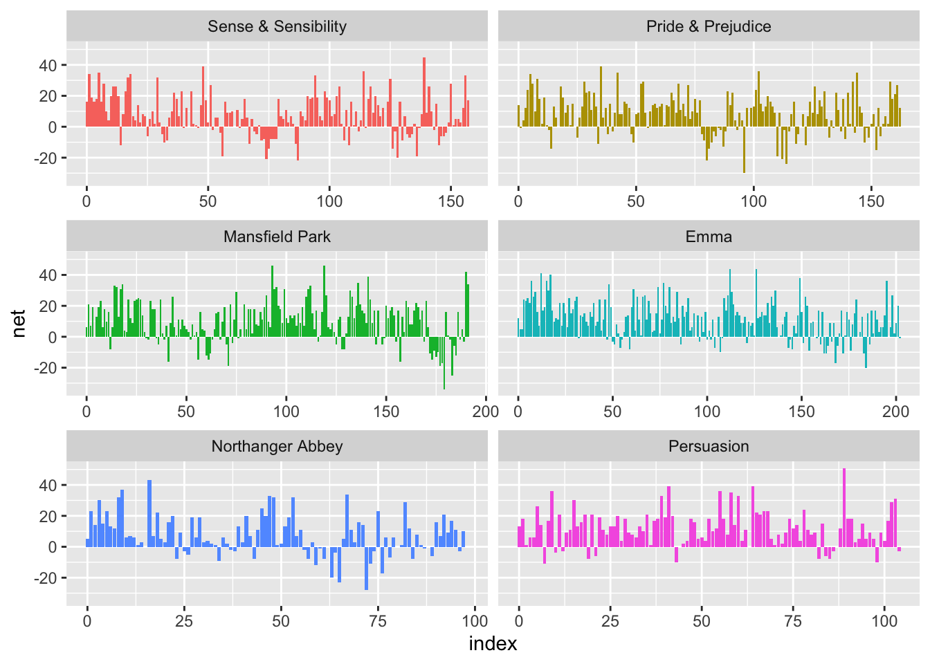
Let’s break up tidy_books into larger blocks of text, say 80 lines long.
We can use the bing lexicon (either positive or negative) to categorize each word within a block.
Recall, the words in tidy_books are in sequential order by line number.
Steps
Use inner_join() to filter out words in tidy_text not in bing while adding the sentiment column from bing
Use count(), and inside the call, create an index variable for the 80-line block of text source for the word while keeping book and sentiment variables
Use index = line_number %/% 80
Note, most blocks will have far fewer than 80 words since we are only keeping the words that are in bing.
Use pivot_wider() on sentiment to get the positive and negative word counts in separate columns and set missing values to 0 with values_fill().
Add a column with the difference in overall block sentiment with net = positive - negative
Plot the net sentiment across each block and facet by book.
Use scales = "free_x" since the books are of different lengths.
We can see the books differ in the number and placement of positive versus negative blocks.
15.8.4 Adjusting Sentiment Lexicons
Consider the Genre/Context for the Sentiment Words. Do they mean what they mean?
These are modern lexicons and 200 year old books.
We should probably look at which words contribute most to the positive and negative sentiment and be sure we want to include them as part of the sentiment.
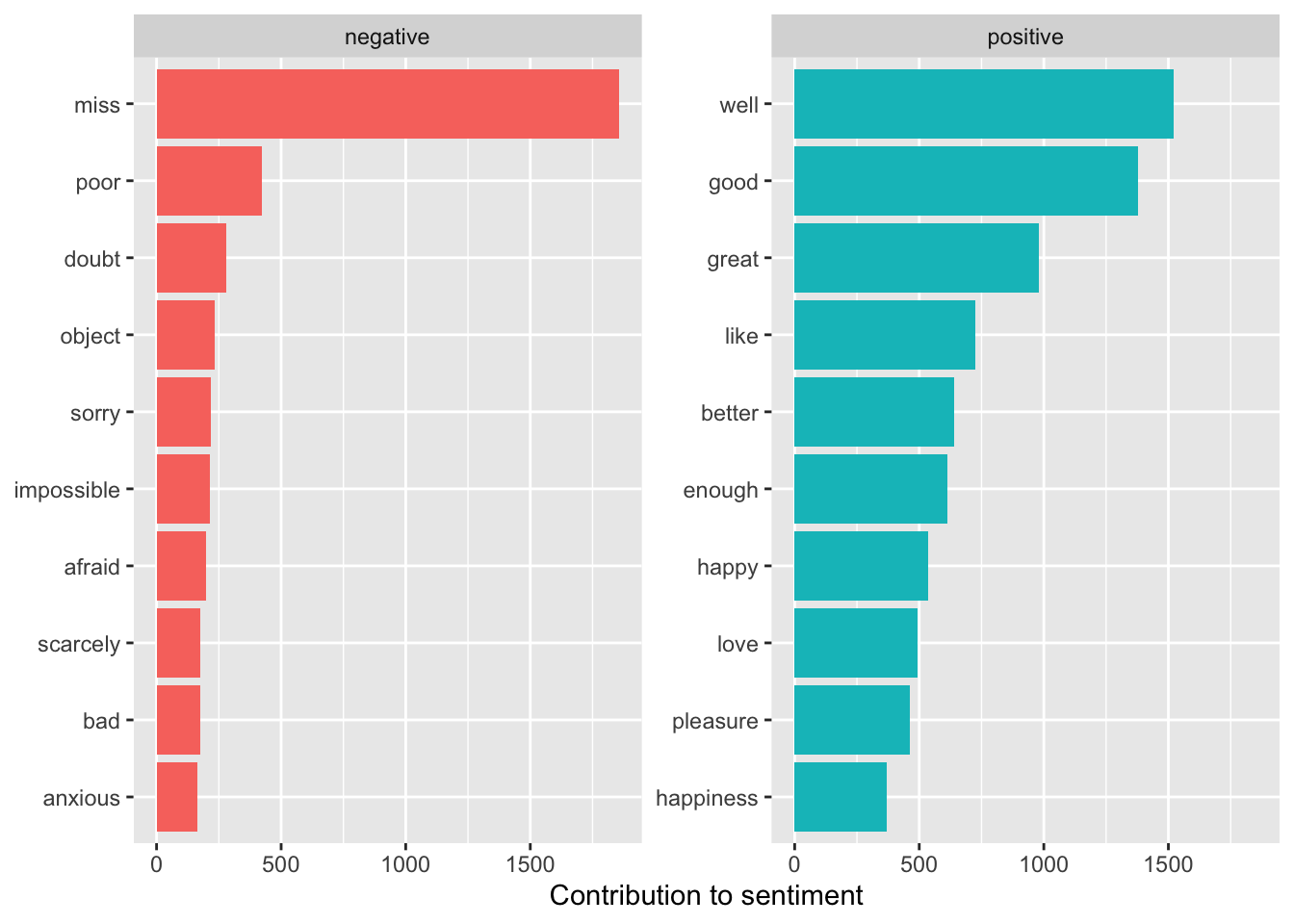
Let’s get the count of the most common words and their sentiment.
tidy_books |>inner_join(get_sentiments("bing"), by ="word",relationship ="many-to-many") |>count(word, sentiment, sort =TRUE) ->bing_word_countsbing_word_counts
# A tibble: 2,585 × 3
   word     sentiment     n
   <chr>    <chr>     <int>
 1 miss     negative   1855
 2 well     positive   1523
 3 good     positive   1380
 4 great    positive    981
 5 like     positive    725
 6 better   positive    639
 7 enough   positive    613
 8 happy    positive    534
 9 love     positive    495
10 pleasure positive    462
# ℹ 2,575 more rows
We can see “miss” might not be a good fit to consider as a negative word given the context/genre.
Let’s plot the top ten, in order, for each sentiment.
bing_word_counts |>group_by(sentiment) |>slice_max(order_by = n, n =10) |>ungroup() |>mutate(word =fct_reorder(word, n)) |>ggplot(aes(word, n, fill = sentiment)) +geom_col(show.legend =FALSE) +facet_wrap(~sentiment, scales ="free_y") +labs(y ="Contribution to sentiment", x =NULL) +coord_flip() +scale_fill_viridis_d(end = .9)
Something seems “amiss” for Jane Austen novels! “Miss” is probably not a negative word, but rather refers to a young woman.
15.8.4.1 Adjusting an Improper Sentiment: Two Approaches
Take the word “miss” out of the data before doing the analysis (add to the stop words), or,
Change the sentiment lexicon to no longer have “miss” as a negative.
15.8.4.1.1Approach 1
Remove “miss” from the text by adding to the stop words data frame and repeating the analysis.
head(stop_words, n =2)
# A tibble: 2 × 2
  word  lexicon
  <chr> <chr>
1 a     SMART
2 a's   SMART
custom_stop_words <-bind_rows(tibble(word =c("miss"), lexicon =c("custom")), stop_words)## SMART is another lexiconhead(custom_stop_words)
# A tibble: 6 × 2
  word  lexicon
  <chr> <chr>
1 miss  custom
2 a     SMART
3 a's   SMART
4 able  SMART
5 about SMART
6 above SMART
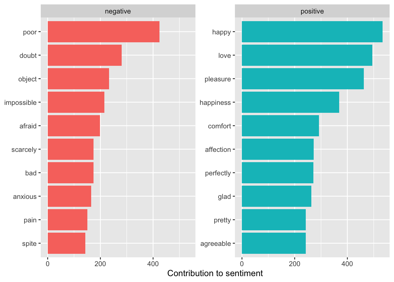
Now let’s redo the analysis with the new stop words.
austen_books() |>group_by(book) |>mutate(linenumber =row_number(),chapter =cumsum(str_detect( text,regex("^chapter [\\divxlc]",ignore_case =TRUE ) )) ) |>ungroup() |>## use word so the inner_join will match with the nrc lexiconunnest_tokens(word, text) |>anti_join(custom_stop_words, by ="word") ->tidy_books_no_misstidy_books_no_miss |>inner_join(get_sentiments("bing"), by ="word",relationship ="many-to-many") |>count(word, sentiment, sort =TRUE) ->bing_word_countshead(bing_word_counts)
# A tibble: 6 × 3
  word      sentiment     n
  <chr>     <chr>     <int>
1 happy     positive    534
2 love      positive    495
3 pleasure  positive    462
4 poor      negative    424
5 happiness positive    369
6 comfort   positive    292
bing_word_counts |>group_by(sentiment) |>slice_max(order_by = n, n =10) |>ungroup() |>mutate(word =fct_reorder(word, n)) |>ggplot(aes(word, n, fill = sentiment)) +geom_col(show.legend =FALSE) +facet_wrap(~sentiment, scales ="free_y") +labs(y ="Contribution to sentiment", x =NULL) +coord_flip() +scale_fill_viridis_d(end = .9)
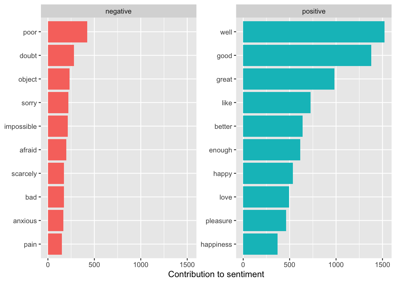
15.8.4.1.2Approach 2
Remove the word “miss” from the bing sentiment lexicon.
We were able to reorder the words above when we were just faceting by sentiment.
If we wanted to see the top five sentiments by book and sentiment instead of just overall across books, we could summarize by facet by both book and sentiment.
# A tibble: 6 × 4
  word  sentiment book                    n
  <chr> <chr>     <fct>               <int>
1 well  positive  Emma                  401
2 good  positive  Emma                  359
3 good  positive  Mansfield Park        326
4 well  positive  Mansfield Park        324
5 great positive  Emma                  264
6 well  positive  Sense & Sensibility   240
## visualize itbing_word_counts |>group_by(book, sentiment) |>slice_max(order_by = n, n =5) |>ungroup() |>mutate(word =fct_reorder(parse_factor(word), n)) |>ggplot(aes(word, n, fill = sentiment)) +geom_col(show.legend =FALSE) +facet_wrap(sentiment ~ book, scales ="free_y") +labs(y ="Contribution to sentiment",x =NULL ) +coord_flip() +scale_fill_viridis_d(end = .9)
Notice the words are now different for each book but are all in the same order, without regard to how often they appear in each book.
All the scales are the same so the negative words are compressed compared to the more common positive words.
There are two new functions in the {tidytext package} to create a different look.
reorder_within(), inside a mutate, allows you to reorder each word by the faceted book and sentiment based on the count.
scale_x_reordered() will then update the x axis to accommodate the new orders.
Use scales = "free" inside the facet_wrap() to allow both x and y scales to vary for each part of the facet.
bing_word_counts |>group_by(book, sentiment) |>slice_max(order_by = n, n =5) |>ungroup() |>mutate(word =reorder_within(word, n, book)) |>ungroup() |>ggplot(aes(word, n, fill = sentiment)) +geom_col(show.legend =FALSE) +facet_wrap(sentiment ~ book, scales ="free") +scale_x_reordered() +scale_y_continuous(expand =c(0, 0)) +labs(y ="Contribution to sentiment",x =NULL ) +coord_flip() +scale_fill_viridis_d(end = .9)
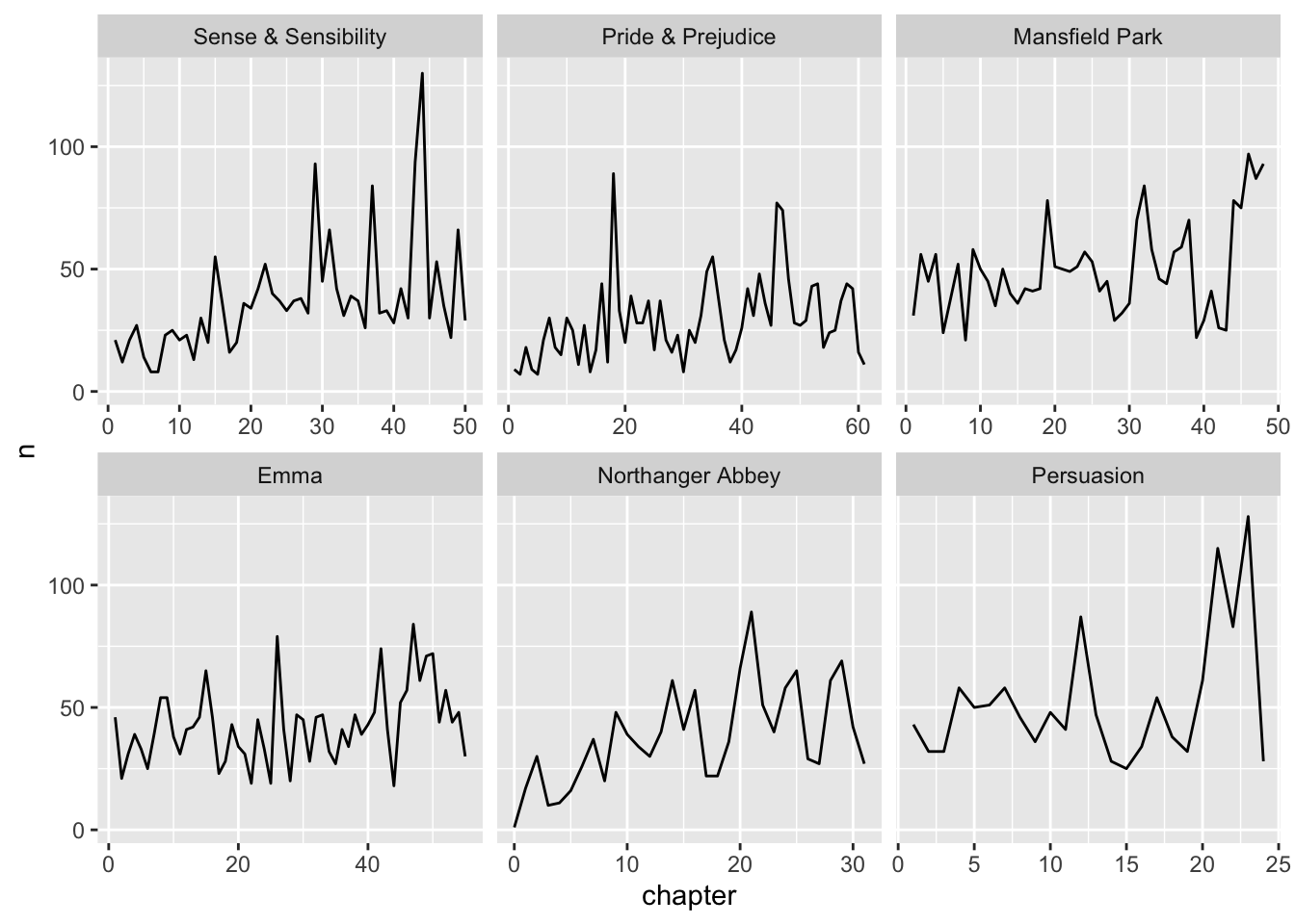
15.8.6 Analyzing Sentences and Chapters
The sentiment analysis we just did was based on single words and so did not consider the presence of modifiers such as “not” which tend to flip the context.
15.8.6.1 Example: Sentence Level
Consider the data set prideprejudice which has the complete text divided into elements of up to about 70 characters each.
If the unit for tokenizing is n-grams, skip_ngrams, sentences, lines, paragraphs, or regex, unnest_tokens() will collapse the entire input together before tokenizing unless collapse = FALSE.
Let’s add a chapter variable and also add a period after the number.
unnest_tokens() separates sentences at periods so we will get rid of periods after Mr., Mrs., and Dr. as a small clean up in addition to separating the chapters headings.
# A tibble: 6 × 5
  book                chapter negativewords words  ratio
  <fct>                 <int>         <int> <int>  <dbl>
1 Sense & Sensibility      43           156  3405 0.0458
2 Pride & Prejudice        34           111  2104 0.0528
3 Mansfield Park           46           161  3685 0.0437
4 Emma                     16            81  1894 0.0428
5 Northanger Abbey         21           143  2982 0.0480
6 Persuasion                4            62  1807 0.0343
These are the chapters with the most negative words in each book, normalized for the number of words in the chapter.
What is happening in these chapters?
In Chapter 43 of Sense and Sensibility Marianne is seriously ill, near death.
In Chapter 34 of Pride and Prejudice, Mr. Darcy proposes for the first time (so badly!).
In Chapter 46 of Mansfield Park, almost the end, everyone learns of Henry’s scandalous adultery.
In Chapter 16 of Emma, she is back at Hartfield after her ride with Mr. Elton, and Emma plunges into self-recrimination as she looks back over the past weeks.
In Chapter 21 of Northanger Abbey, Catherine is deep in her Gothic faux-fantasy of murder, etc..
In Chapter 4 of Persuasion, the reader gets the full flashback of Anne refusing Captain Wentworth and sees how sad she was and now realizes it was a terrible mistake.
We have seen multiple ways to use sentiment analysis in single words and large blocks of text to analyze the flow of sentiment within and across large works of text.
The same concepts and techniques can work with analyzing Reddit comments, tweets, Yelp reviews, etc..
15.9 Word Cloud Plots
Word clouds are a popular way to display word frequencies, but they are best viewed as an informal or exploratory visualization rather than a strong statistical graphic.
The {wordcloud} package (Fellows (2018)) uses base R graphics to create word clouds.
It includes functions to create “commonality clouds” or “comparison clouds” for comparing words across multiple documents.
Install the package using the console and load it into your file.
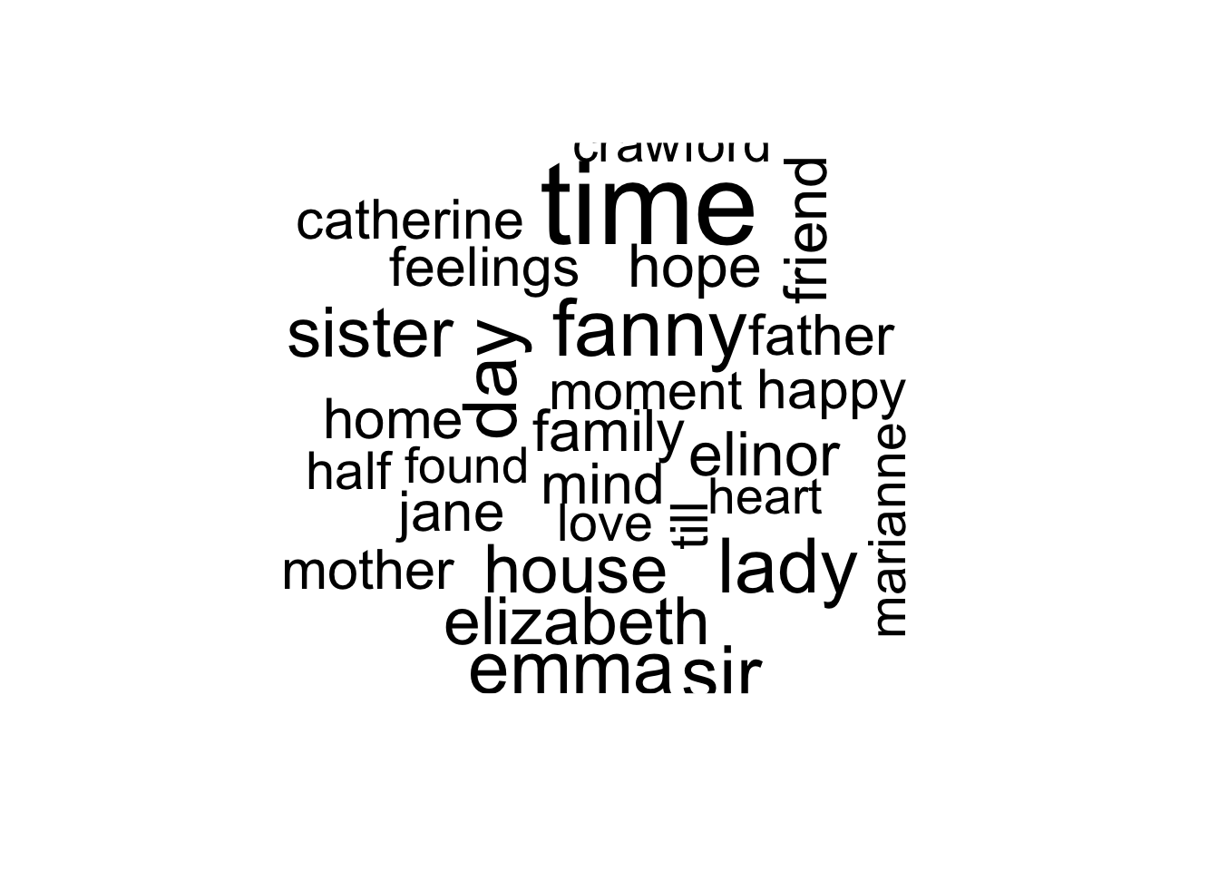
Let’s create a word cloud of tidy_books without the stop words.
library(wordcloud)tidy_books |>anti_join(stop_words, by ="word") |>count(word) |>with(wordcloud(word, n, max.words =30))
## Custom stop words - no misstidy_books |>anti_join(custom_stop_words, by ="word") |>count(word) |>with(wordcloud(word, n, max.words =30))
Word clouds are easy to make and are still widely used, but they have important limitations.
They make precise comparisons difficult because there is no common axis.
They emphasize visual impression over exact values.
They are less useful when you want to compare frequencies across books, authors, or sentiments.
For text analysis, more informative alternatives often include:
sorted bar charts or lollipop plots for the most frequent words
faceted bar charts for comparing top words across books or sentiment groups
heatmaps for word presence or weighted frequencies across documents
scatterplots for comparing relative frequencies across corpora
network plots for word pairs or co-occurrence relationships
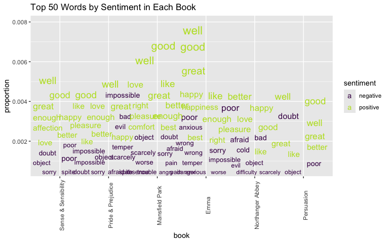
A Chatter Plot has more information about the presence of words than font size.
Try a repeat of top 50 Jane Austen words by sentiment and books.
library(ggrepel) ## to help words "repel each othertidy_books |>inner_join(bing_no_miss, by ="word",relationship ="many-to-many") |>count(book, word, sentiment, sort =TRUE) |>mutate(proportion = n /sum(n)) |>group_by(sentiment) |>slice_max(order_by = n, n =50) |>ungroup() ->tempptempp |>ggplot(aes(book, proportion, label = word)) +## ggrepel geom, make arrows transparent, color by rank, size by ngeom_text_repel(segment.alpha =0,aes(color = sentiment, size = proportion,## fontface = as.numeric(as.factor(book)) ),max.overlaps =50 ) +## set word size range & turn off legendscale_size_continuous(range =c(3, 6), guide ="none") +theme(axis.text.x =element_text(angle =90)) +ggtitle("Top 50 Words by Sentiment in Each Book") +scale_color_viridis_d(end = .9)
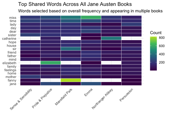
Another useful alternative is a heatmap, which allows us to compare the frequency of words across multiple documents using a common color scale.
Heatmaps are particularly helpful when:
comparing many words across multiple books or authors
identifying which words are especially common in some documents but not others
showing patterns that may be harder to see in bar charts
In this example, we use raw word counts. Next week, we will revisit this idea using tf-idf, which helps highlight words that are not just frequent, but especially distinctive to a given document.
To focus the display on more interpretable patterns, we first remove stop words and count the remaining words by book.
We then restrict the analysis to words that appear in at least three books so that the heatmaps emphasize shared vocabulary rather than words unique to a single text.
Finally, we compare two perspectives: a global view based on the most common shared words across all books, and a within-book view based on the most common shared words within each book.
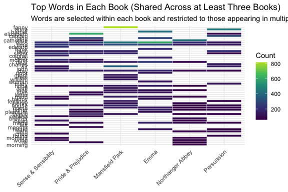
# Step 1: count non-stop words by bookword_counts <- tidy_books |>anti_join(stop_words, by ="word") |>count(book, word)# Step 2: identify words that appear in at least 3 booksshared_words <- word_counts |>group_by(word) |>summarize(n_books =n_distinct(book), .groups ="drop") |>filter(n_books >=3)# Step 3: get top shared words overall (not per book)top_words <- word_counts |>semi_join(shared_words, by ="word") |>group_by(word) |>summarize(total =sum(n), .groups ="drop") |>slice_max(order_by = total, n =20) |>pull(word)# Step 4: plot all books for those globally selected wordsword_counts |>filter(word %in% top_words) |>ggplot(aes(x = book, y =fct_reorder(word, n), fill = n)) +geom_tile(color ="white") +scale_fill_viridis_c(end = .9) +labs(title ="Top Shared Words Across All Jane Austen Books",subtitle ="Words selected based on overall frequency and appearing in multiple books",x =NULL,y =NULL,fill ="Count" ) +theme_minimal() +theme(axis.text.x =element_text(angle =45, hjust =1))# Step 5: get top shared words within each booktop_shared_words <- word_counts |>semi_join(shared_words, by ="word") |>group_by(book) |>slice_max(order_by = n, n =20) |>ungroup()# Step 6: plot top shared words within each booktop_shared_words |>ggplot(aes(x = book, y =fct_reorder(word, n), fill = n)) +geom_tile(color ="white") +scale_fill_viridis_c(end = .9) +labs(title ="Top Words in Each Book (Shared Across at Least Three Books)",subtitle ="Words are selected within each book and restricted to those appearing in multiple books",x =NULL,y =NULL,fill ="Count" ) +theme_minimal() +theme(axis.text.x =element_text(angle =45, hjust =1))
The two plots use different selection strategies:
The first selects top words across all books (global comparison)
The second selects top words within each book (local comparison). A word may appear in at least three books overall but still be shown in only some books here, because the plot keeps only the top words within each individual book.
This distinction affects how patterns should be interpreted.
At times, you may be asked to create a word cloud, and it is straightforward to do so.
However, word clouds are usually better for quick visual summaries than for analysis.
When you need clearer comparisons or more interpretable results, bar charts, faceted comparisons, heatmaps, scatterplots, or network plots are often better choices.
Robinson, David, and Myfanwy Johnston. 2023. Gutenbergr: Download and Process Public Domain Works from Project Gutenberg. https://docs.ropensci.org/gutenbergr/.
Silge, Julia, and David Robinson. 2016. “Tidytext: Text Mining and Analysis Using Tidy Data Principles in R.”The Open Journal JOSS 1 (3). https://doi.org/10.21105/joss.00037.