10  Generative AI Models

Keywords

ollama, LLM, Prompting, Sentiment analysis, Stop Words

10.1 Introduction

This module investigates multiple large language models to understand how they interact with prompts and use probabilistic methods to generate responses.

Learning Outcomes

• Use Ollama to download LLMs to a local computer
• Interact with the LLMs and analyze the outputs.
• Use {tidytext} functions for basic natural language processing text analysis.

10.1.1 References

• Ollama (Ollama 2025)
• Ollama GitHub Repository
• Text Analysis with the {tidytext} package (Silge and Robinson 2023)

10.2 Getting Large Language Models onto Your Computer

ollama is a free, open-source tool that lets you download and run large language models (LLMs) locally on your own machine.

All ollama commands in this chapter are run in a local terminal window (macOS Terminal, Windows PowerShell / WSL2, or Linux shell).

• The R code chunks that follow work with text you copy-paste from that terminal into Posit Cloud.

10.2.1 Installing ollama

Go to https://ollama.com, download the installer for your OS, and run it.

Verify it installed correctly:

ollama --version

10.2.2 Starting the ollama Server

ollama serve

Leave that terminal tab open. Open a second terminal tab for the commands below.

10.2.3 Downloading Models

# Small model (~500 MB) — good for quick experiments
ollama pull qwen2.5:0.5b

# Medium model (~4 GB) — better quality, needs at least 8 GB RAM
ollama pull llama3

10.2.4 Listing Installed Models

ollama list

Output will look similar to:

NAME                ID              SIZE    MODIFIED
llama3:latest       365c0bd3c000    4.7 GB  2 days ago
qwen2.5:0.5b        a8b0c5157701    394 MB  3 days ago

10.3 Basic Prompting

Talk to a model directly from the terminal:

ollama run llama3 "Hey, is this thing on?"
ollama run llama3 "こんにちは"

10.3.1 Capturing Terminal Output in R

Since ollama runs locally and R runs in Posit Cloud, the bridge is copy and paste:

1. Run the ollama command in your local terminal.
2. Copy the model response.
3. Paste it as a string in the R chunk in Posit Cloud.

10.4 Exploring How LLMs Work

See how the model completes a partial word:

ollama run llama3 "Compu"

The model splices your prompt into a template before feeding it to the predictive model. Look at the template:

ollama show llama3 --modelfile

The TEMPLATE section uses Go template syntax (https://pkg.go.dev/text/template).

• { .TEXT_GOES_HERE } marks where your prompt is inserted.

Deepseek-r1 uses a different style template:

ollama show deepseek-r1 --modelfile | less

Templates are supposed to be hidden from the user, but sometimes they escape!

Duolingo’s Lily is acting a little weird

After templating, the prompt is fed to a predictive text model that samples from a conditional probability distribution:

\[ p(t_{n+1} | t_n, t_{n-1}, ..., t_1) \tag{10.1}\]

10.4.1 Non-Determinism: Run the Same Prompt Five Times

# Run this five times — observe how completions differ each time
ollama run llama3 "What"

Copy each of the five responses and paste them into the R chunk below.

library(tidyverse)
library(tidytext)
# Copy output from your terminal and paste it into the R chunks below.

# Run: ollama run llama3 "What"  five times in your local terminal.
# Paste each response as one string in the vector below.
raw_runs <- c(
  "It seems like you might have started to ask a question, but it got cut off! Can you please rephrase or complete your question? I'm here to help with any questions you might have.",
  "It seems like you've started to ask a question, but it's cut off! What were you wondering about? I'm here to help with any questions or topics you'd like to discuss.",
  "It seems like you may have started to ask a question, but it got cut off! Can you please rephrase or complete your question? I'm here to help with any inquiry you might have.",
  "It seems like you started to ask a question, but it got cut off! Could you please finish your question or clarify what's on your mind? I'm here to help with any topic or inquiry you might have.",
  "It seems like you might have started to ask a question, but it got cut off! Could you please rephrase or complete your question? I'm here to help and want to make sure I understand what you're asking.."
)

tibble(run = seq_along(raw_runs), response = raw_runs)

# A tibble: 5 × 2
    run response                                                                
  <int> <chr>                                                                   
1     1 It seems like you might have started to ask a question, but it got cut …
2     2 It seems like you've started to ask a question, but it's cut off! What …
3     3 It seems like you may have started to ask a question, but it got cut of…
4     4 It seems like you started to ask a question, but it got cut off! Could …
5     5 It seems like you might have started to ask a question, but it got cut …

10.4.2 Start an Interactive Session

So far we have provided a model and a prompt and gotten a response.

Now let’s start an interactive session with a model.

• You should see the cursor change to >>>.
• When ready to exit use /bye.

ollama run llama3 

10.4.3 Temperature: Controlling Randomness

You can reduce randomness by lowering the temperature parameter.

• temperature = 0 makes the model more deterministic or factual.
• Set the temperature to 0 (inside the interactive session with: /set parameter temperature 0

/set parameter temperature 0

Possible Single Prompts

• Design a new species of animal that might live on the Moon or another plant and describe in two sentences
• Identify a theme and identify 5 places to visit in Albania for a wild and crazy time using less than 50 words.
• Write a haiku where every word starts with the letter s.

Repeat a few times.

Now set the temperature to 1

/set parameter temperature 1

Repeat a few times. - Do you notice a difference?

Now ask the model directly how it might behave at the two settings.

Prompt 1: Storytelling

• Imagine I ask you to tell me a story about a llama. If I set the creativity level to 0, what kind of story would you tell? Would it be straightforward and factual?
• Now, if I set the creativity level to 1, how might your story change? Would it be more imaginative or fantastical?

Prompt 2: Word Association

• Think about a word like “cloud”. If I set the creativity level to 0, what words would you associate with it? Would they be related to weather or something else?
• Now, if I set the creativity level to 1, how might your associations change? Would you come up with more abstract or creative connections?

Prompt 3: Poetry

• Imagine I ask you to write a short poem about a sunset. If I set the creativity level to 0, what kind of poem would you write? Would it be descriptive and factual?
• Now, if I set the creativity level to 1, how might your poem change? Would it be more lyrical or metaphorical?

Exit the session with /bye.

10.5 A Guide to Prompt Engineering

As we have just seen, interacting with generative models is all about the prompts.

The field of Prompt Engineering has evolved to help users interact more systematically and effectively LLMs.

Note

This section was written based on a conversation with an AI Assistant that started with a 156 word prompt and about 25 follow-up prompts to adjust, expand and refine content. Additional human editing improved clarity and consistency as well as formatting and adjustments to code and code chunk options. References were checked and adjusted for accuracy and citations were added. Links to inline references were added. Any errors are my responsibility.

10.5.1 Prompt Engineering

“Prompt engineering is the process of writing effective instructions for a model, such that it consistently generates content that meets your requirements.” OpenAI (2025)

A “prompt” can be a question, a request for code, a set of instructions, or even an ongoing conversation with a Large Language Model an LLM.

• Creating or “engineering” a prompt (or series of prompts) to produce the most accurate, useful, and relevant output possible to meet your goals is still a mix of art and science.

Prompt engineering builds on an understanding of how LLMs work (not how they are trained) to create prompts that are effective for your purposes.

The following characteristics of LLMs shape how one engineers effective prompts.

• Non-determinism: LLM responses vary because they are generated from probabilities in a high-dimensional space. Small wording changes can produce very different outputs.
  • Asking what is the “most positive” versus the “least negative” sentiment of text.
• Context Sensitivity: LLMs don’t “understand” in the human sense; they generate responses based on patterns in data. How you ask a question strongly influences the quality of the answer.
  • Specifying “Give me R code” versus “Explain in plain English” leads to very different outputs.

You can apply guidelines and best practices to improve your chances of getting useful results consistently while building your understanding and skills.

• Efficiency: A well-crafted prompt reduces the need for repeated clarifications.
• Accuracy: Clear context, guidance, examples, and constraints can help minimize errors or hallucinations.
• Improved Collaboration: prompt engineering can be seen as refining or debugging your question prior to collaborating with others or the LLM.
• Multi-language skill: The same techniques apply whether you’re generating R code, Python code, documentation, or explanations.

In short: Prompt engineering is about learning how to “talk to the model” effectively so it can become a productive tool for your goals rather than a source of confusion.

10.5.2 How LLMs Respond to Prompts

LLMs (like ChatGPT, Claude, or Gemini) do not “understand” like humans. Instead, they:

1. Predict the next token (word or subword) given your prompt’s input and context.
2. Use patterns from training data to approximate reasoning.
3. Are sensitive to framing: wording, order, specificity, and constraints change the output.
4. Can hallucinate: generate confident-sounding but false statements.

10.5.2.1 Tokenization

LLMs do not read raw text directly. Instead, they break text into tokens (smaller units such as words, subwords, or characters).

• Tokens are not always whole words.
  • Example: "data science" → ["data", " science"] (2 tokens)
    
  • Example: "statistics101" → ["statistics", "101"] (2 tokens)
    
  • Example: "internationalization" → ["international", "ization"] (2 tokens)
• This is similar to but not the same as Lemmatization which reduces words to their base form (common in NLP preprocessing, not in LLM tokenization).
  • "running" → "run"
    
  • "better" → "good"

Here is a toy example of token splitting.

                  Word                  Tokens
1                 data                    data
2        statistics101        statistics | 101
3 internationalization international | ization
4              running              run | ning
5               better                  better

10.5.2.2 The Context Window and Token Limits and Conversation Context

The context window is the full set of tokens the model sees at any single moment; think of it as the model’s working memory for a task.

• It holds everything at once: your system instructions, the conversation history, your current message, and any retrieved documents or data.
• The model can only reason about what is currently in this window.
  • Nothing outside it exists from the model’s perspective.
• Managing what goes into this window (what to include, what to summarize, what to leave out) becomes one of the most important skills as you move from interactive chat toward writing code that calls models programmatically.

Each model has a maximum token limit (prompt + response combined).

• Context windows have grown dramatically and continue to expand rapidly so always check the current documentation for the model you are using.
• Representative sizes as of early 2026:
  • Small/local models (e.g., ollama 7B–13B): 8k–32k tokens
  • Mid-range models (e.g., GPT-4o, Llama 3.1): 128k tokens
  • Large frontier models (e.g., Claude Sonnet 4.6, Gemini 3 Pro, GPT-5.4): 200k–1M+ tokens

How “memory” actually works in interactive chat:

• The model itself is stateless, i.e.,it has no built-in memory between calls.
• Each prompt is processed independently, with no knowledge of prior exchanges unless that history is explicitly included.
• The appearance of a continuous conversation is an illusion created by the application layer (Claude.ai, ChatGPT, etc.), which automatically prepends all prior messages to each new prompt before sending it to the model.
• As a conversation grows, so does the context it consumes.
• Long conversations with code in prompts and responses can fill the context window quickly and slow performance.
• If the limit is approached, older context may be truncated, leading to loss of information or inconsistent responses and eventually you will need to start a new conversation.

Bigger is not always better — context rot:

• Research consistently shows that model performance degrades as context length increases, even when the tokens technically fit in the window. This is sometimes called context rot.
• Models tend to attend more reliably to information near the beginning or end of the context, and may lose track of details buried in the middle.
• More tokens can mean more distraction, not more capability.
• A practical rule of thumb: effective reliable performance is typically lower than the advertised maximum.

TipBest practices to manage your context window

• Keep prompts focused. Paste only the relevant portion of a dataset or file, not the whole thing. Summarize or sample when the input is large.
• Start a new conversation for a new topic. This prevents unrelated context from accumulating and keeps the window clean.
• For local models with smaller windows (as you will use with ollama), this constraint is tighter so short, targeted prompts matter more.
• Place the most important information at the beginning of your prompt, not buried in the middle, where attention is weakest.

10.5.2.3 Tokens are Converted to Numbers

• LLMs do not operate on tokens as text. Each token is mapped to a numerical vector (an embedding).
  
• Embeddings are high-dimensional vector representations of tokens or text that capture semantic meaning.
• LLM embeddings are vectors with hundreds or thousands of dimensions, not just 2 or 3, and each dimension encodes some aspect of meaning, context, or syntactic/semantic feature.
  • Different models can use different embedding schemes.
• The model performs mathematical operations on these vectors to predict the next token based on mathematical similarity or “closeness.”

Example:
- "dog" → [0.12, -0.03, 0.88, ...]
- "puppy" → [0.14, -0.01, 0.91, ...]
- "car" → [0.80, 0.20, -0.05, ...]

10.5.3 Measuring Closeness

Similarity between the embedding vectors is measured using metrics like cosine similarity.

\[ \text{cosine similarity} = \frac{\vec{A} \cdot \vec{B}}{\|\vec{A}\| \|\vec{B}\|} \]

• Cosine similarity = 1 -> vectors point in the same direction (highly similar meaning).
  
• Cosine similarity = 0 ->vectors are orthogonal (unrelated meaning).

Embeddings allow LLMs to “understand” similar words or phrases as they have embeddings “close” together in vector space.

• These metrics are used for:
  • Semantic search (finding relevant text)
    
  • Retrieval-Augmented Generation (RAG)
    
  • Clustering or similarity calculations

10.5.4 Visualizing Embeddings in R

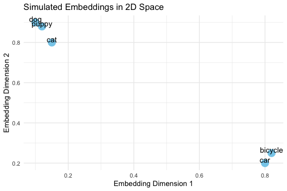
This example shows how words with similar meaning might cluster together in the embedding space.

• “dog”, “puppy”, and “cat” cluster closely, reflecting semantic similarity.
• “car” and “bicycle” are farther away, showing unrelated meaning.
• In real embeddings, vectors are high-dimensional, but this 2D example illustrates the concept.
• Cosine similarity measures closeness mathematically in high dimensions, even though they can’t be plotted.

Warning

Important nuance

• These similarity measures are inherently fuzzy.
  
• Minor variations in your prompt—such as negating a sentence, reordering words, or changing context—can result in large differences in the output, even if the overall meaning seems similar to a human reader.

Example:
- Prompt 1: "List three common R functions for plotting a histogram."
- Prompt 2: "List three widely-used R functions for plotting a histogram."
- Prompt 3: "List three popular R functions for plotting a histogram."

Even though only one word changes, the model may:

• Suggest completely different functions.
• Reorder examples differently.
• Include/exclude certain packages.

This happens because embeddings map text to points in a continuous space, and the model predicts outputs based on small differences in those positions.

Takeaway: Always experiment with multiple phrasings and verify results. Treat embeddings and similarity measures as guides, not exact truth.

10.5.5 Guidelines for Effective Prompts

Good prompts share a few common traits: they are clear, contextual, and iterative. Here are strategies to improve your interactions with AI tools:

• Be Specific
  Clearly describe what you want the AI to do. Include the programming language, the type of output, and the level of detail you expect.
  Example:
  • Weak: “Plot the data.”
  • Strong: “Write R code using ggplot2 to create a line plot of revenue by year with labeled axes and a descriptive title.”
• Give Context
  Provide background information such as the data structure, libraries, or your end goal. This reduces ambiguity and helps the AI tailor its response.
  Example:
  • “I have a pandas data frame with columns city and population. Please write Python code using seaborn to create a bar chart of population by city.”
• State Constraints
  Specify limitations or requirements for the response, such as the format, length, or assumptions.
  Example:
  • “Give me only the R code, no explanations.”
  • “Limit the answer to a single ggplot2 figure.”
  • “Assume the data frame has no missing values.”
• Iterate
  Think of prompting as a conversation, not a one-shot request. Start simple, review the output, and refine with follow-up prompts.
  Example:
  • First prompt: “Write Python code to read a CSV file and display the first five rows.”
  • Follow-up: “Now extend this code to calculate the mean of all numeric columns.”
  • Next follow-up: “Format the summary as a neat table.”
  • Later, we will see how iteration moves from conversation to code, where you can reuse a prompt programmatically rather than by typing.
• Verify
  Never assume the AI is correct. Check the output against your own knowledge, official documentation, or by running the code. Be alert for hallucinations (nonexistent functions, incorrect syntax, or misleading explanations).
  Example:
  • If the AI suggests robust_cor() in R, search the documentation. If it doesn’t exist, redirect:
    “That function doesn’t exist. Could you instead use Spearman’s correlation or show me how to fit a robust regression with MASS::rlm()?”
• Adjust for Creativity or Accuracy
  You can control how wide-ranging or precise the response should be by adjusting your wording.
  Example:
  • Creative: “Show three different ways in R to visualize a distribution.”
  • Accurate: “Show the single most standard ggplot2 approach for plotting a histogram of a numeric variable.”
• Assign a Role
  Guide the style of the response by telling the AI who it should act as.
  Example:
  • “You are a data science tutor. Explain correlation to a beginner and include an R code example.”
  • “You are a coding assistant. Provide concise Python code with no explanations.”

10.5.5.1 Example: Making a Good First Prompt

Weak prompt:
> Plot the data.

Improved prompt:
> I have a data frame in R with columns year and revenue. Please write R code using ggplot2 to create a line plot of revenue by year, with labeled axes and a title.

Here is a sample response.

# Load ggplot2 library
library(ggplot2)

# Create sample data frame (replace with your own data)
df <- data.frame(year = c(2010, 2011, 2012, 2013, 2014),
                 revenue = c(10000, 12000, 14000, 16000, 18000))

# Create the plot
ggplot(df, aes(x = year, y = revenue)) + 
  geom_line() + 
  labs(title = "Revenue by Year", x = "Year", y = "Revenue")
# Print the plot
print(ggplot(df, aes(x = year, y = revenue)) + 
      geom_line() + 
      labs(title = "Revenue by Year", x = "Year", y = "Revenue"))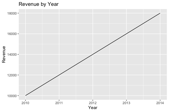

10.5.5.2 Example: Building a Conversation

First Prompt:
> Write Python code to read a CSV and summarize the first five rows.

LLM Output:
Code using pandas.read_csv() and df.head().

Follow-Up Prompt:
> Please extend your code to also compute the mean of all numeric columns and print the result.

LLM Output:
Adds df.mean(numeric_only=True).

Next Follow-Up:
> Could you format the summary as a table with column means below the head output?

The model refines until the solution fits your needs.

10.5.5.3 Example: Checking for Hallucinations

Prompt:
> Write R code to compute a robust correlation coefficient.

LLM Output:
Provides code with a function robust_cor() (a hallucination as the function does not exist).

Student Check: Gets an error message and looks up if robust_cor() exists in R.
- If not, ask:
> That function doesn’t seem to exist. Could you instead show how to use MASS::rlm() or another real package to compute robust correlation?

The key is to verify and redirect.

10.5.5.4 Example: Large vs. Small Model Responses

The same prompt can yield different results depending on the size of the model.

Larger models (billions of parameters) generally produce more detailed and accurate answers, while smaller ones may be faster but less reliable.

Prompt:
> In R, how do I compute the correlation between two variables when the data has outliers?

Model	Response
Large model (e.g., GPT-4, Claude Opus, Llama-70B)	“One option is to use a robust correlation method. For example, you can use Spearman’s rank correlation in R: cor(x, y, method = "spearman"). Another approach is to fit a robust regression using MASS::rlm() if you want to downweight outliers. Both approaches reduce the influence of extreme values compared to Pearson correlation.”
Smaller model (e.g., GPT-3.5, Llama-7B)	“You can use cor(x, y) in R. This computes correlation between two vectors.” (Note: does not mention outliers or alternatives like Spearman or robust regression.)

Takeaway:
- The large model recognizes the nuance (outliers) and suggests multiple valid approaches.
- The smaller model gives a quick but incomplete response.
- Lesson: Always check whether the model has considered your context.

10.5.5.5 Example: Specifying Roles

When prompting, you can assign a role to the AI which will adjust its response.

Prompt 1 (role: assistant):
> You are a coding assistant. Write R code to plot the distribution of a numeric variable.

Likely Response:
Straightforward R code using hist() or ggplot2::geom_histogram().

Prompt 2 (role: instructor):
> You are a statistics instructor. Explain to a beginner how to plot the distribution of a numeric variable in R, and include an example using ggplot2.

Likely Response:
A step-by-step explanation with annotated code — more teaching-oriented.

10.5.5.6 Example: Adjusting Creativity vs. Accuracy

LLMs can be “dialed” for creativity (diverse answers, new ideas) or accuracy (precise, more deterministic answers).

• This is often controlled by a setting called temperature (higher = more creative, lower = more predictable).
  
• Even without changing system settings, you can influence style through your prompt wording.

Prompt (creative mode):
> Be imaginative. Show me three different R approaches to visualize the distribution of a variable.

Possible Output:
- Histogram (geom_histogram())
- Density plot (geom_density())
- Boxplot (geom_boxplot())

Prompt (accuracy mode):
> Provide the single most standard way in R using ggplot2 to visualize a variable’s distribution.

Possible Output:
One clean example using geom_histogram(), without alternatives.

Below we show a “standard” accurate plot of a distribution: If the AI had been asked in creative mode, it might instead show a density plot, violin plot, or boxplot.

library(ggplot2)
set.seed(42)

values <- rnorm(200, mean = 50, sd = 10)

ggplot(data.frame(values), aes(x = values)) +
  geom_histogram(binwidth = 5, fill = "skyblue", color = "black") +
  labs(title = "Distribution of Values (Accurate Mode)",
       x = "Value", y = "Count") +
  theme_minimal()

You can shape the AI’s “persona”(assistant, instructor, critic, tutor) and also control breadth vs. precision of answers depending on their goals.

10.5.6 Summary

Here is a quick reference sheet you can use when working with AI tools:

Strategy	What It Means	Example Prompt
Specify Role	Tell the AI who it should act as (assistant, instructor, critic, tutor).	“You are a statistics instructor. Explain correlation to a beginner with examples in R.”
Give Context	Provide background: dataset, libraries, goals.	“I have a data frame in R with columns year and revenue. Use ggplot2 to plot revenue by year.”
State Constraints	Limit length, format, or assumptions.	“Give me Python code only, no explanations, using pandas and seaborn.”
Iterate	Use follow-up prompts to refine or extend.	“Now add labels to the axes.”
Verify	Check outputs against your knowledge or documentation.	“That function doesn’t exist in R. Show me an alternative from MASS or robustbase.”
Creativity vs. Accuracy	Ask for one best method (accuracy) or multiple diverse methods (creativity).	“Show three different ways in R to visualize a distribution.”
Check for Hallucination	Be skeptical if the AI invents code/functions. Redirect if necessary.	“I can’t find that function. Can you cite the package or suggest a real function?”

Prompt engineering is not about tricking the AI, but about effective communication.

Think of the AI as a partner:  - You provide structure, clarity, and verification. - It provides suggestions, alternatives, and explanations.

With practice, you’ll learn when to ask for creativity, when to demand precision, and how to iterate toward a reliable solution.

In the next section, we begin moving from interactive conversations to code driven interactions, turning prompts from typed messages into functions that can be called, tested, and reused.

10.6 Basic Text Cleanup

LLMs are a convenient source of raw material for natural language processing methods. Let’s ask for one of the LLMs to write us a poem to play with!

ollama run llama3 "Write a sonnet in the style of Shakespeare"

Here’s the poem it made.

Fairest of maidens, with eyes so bright,
Like stars that shine in darkness, thou dost light
The path for love to follow, and thy face
Doth glow with beauty, like the morning's grace.

Thy tresses, golden threads of finest spun,
Do hang in curls, like ivy on a sun
Kissed rock, and on thy lips, a smile is won
That doth entice, as honey to the bee.

But alas, fair maiden, thou art not mine own,
For thou dost shine with beauty, all my own
And I, but dust, a fleeting moment's sigh
Do seek to grasp thee, and be gone.

Yet still, I'll cherish every fleeting glance,
And hope that fate may bring us to one dance.

Note: A traditional Shakespearean sonnet consists of 14 lines, with a rhyme scheme of ABAB CDCD EFEF GG. This sonnet follows that structure.

The formatting turns out to be unhelpful if you want to study word usage. So let’s strip out all the punctuation, flatten the case, and make each word a single row.

sample_text <- "Fairest of maidens, with eyes so bright,
Like stars that shine in darkness, thou dost light
The path for love to follow, and thy face
Doth glow with beauty, like the morning's grace.

Thy tresses, golden threads of finest spun,
Do hang in curls, like ivy on a sun
Kissed rock, and on thy lips, a smile is won
That doth entice, as honey to the bee.

But alas, fair maiden, thou art not mine own,
For thou dost shine with beauty, all my own
And I, but dust, a fleeting moment's sigh
Do seek to grasp thee, and be gone.

Yet still, I'll cherish every fleeting glance,
And hope that fate may bring us to one dance.

Note: A traditional Shakespearean sonnet consists of 14 lines, with a rhyme scheme of ABAB CDCD EFEF GG. This sonnet follows that structure."
poem_tidied <- tibble(poem = sample_text) |>
  unnest_tokens(word, poem )

Have a look at the resulting data frame! You’ll notice that there’s one column, called word.

• If you wanted to call the column something else, you’d replace the word in the line above with whatever you wanted to call it.
• But most of the tidy text mining tools expect word as the column of words, so we’ll use that.

Note that unnest_tokens() did a few other things as well. Can you figure out what these are?

OK, let’s count the words! You can do this in several ways depending on what you want to see.

count(poem_tidied, word)

# A tibble: 101 × 2
   word       n
   <chr>  <int>
 1 14         1
 2 a          5
 3 abab       1
 4 alas       1
 5 all        1
 6 and        5
 7 art        1
 8 as         1
 9 be         1
10 beauty     2
# ℹ 91 more rows

or try

poem_tidied |> count(word, sort = TRUE)

# A tibble: 101 × 2
   word      n
   <chr> <int>
 1 a         5
 2 and       5
 3 of        4
 4 that      4
 5 to        4
 6 with      4
 7 like      3
 8 the       3
 9 thou      3
10 thy       3
# ℹ 91 more rows

Look closely at the word frequencies you just produced. Can you explain why some words are more common?

• Some of them just aren’t very informative, since they’re words like “my”, “a”, and such.
  • Linguists call these “stop words,” and we’d like to get rid of them for most of our analysis.
    
• Now, an important question is whether you want to get rid of them, or not get rid of them. Probably the latter, I’m thinking, because there might be some situations where they’re useful. Hold that thought.

One of the things loaded when you brought in the {tidytext} library was a list of modern English stop words in the table stop_words.

stop_words

# A tibble: 1,149 × 2
   word        lexicon
   <chr>       <chr>  
 1 a           SMART  
 2 a's         SMART  
 3 able        SMART  
 4 about       SMART  
 5 above       SMART  
 6 according   SMART  
 7 accordingly SMART  
 8 across      SMART  
 9 actually    SMART  
10 after       SMART  
# ℹ 1,139 more rows

Coming back to the task of removing stop words, what we have is a table poem_tidied, in which there is one column called word, and many rows, one for each word.

We want to remove (temporarily) each row that has a word that’s in the stop_words table.

• If you were writing this in Java or Python, you’d probably use a loop to do that.
  
• But R makes this process a snap with something called an anti-join. Specifically, an anti-join takes two tables and removes all the rows in the first table according to a matching rule that’s built from the second table.
  
• This rule matches up two columns – usually called keys – one from each table. (As you might expect, there’s also a join as well that puts two tables together.)

Aside: if you read the documentation for anti_join, you’ll probably find that it’s a bit mysterious. That’s because anti_join is a generic function, and can do lots of other matching rules, and various other kinds of tricks too! It’s very useful!

OK, enough theory. Let’s get rid of those stop words!

poem_tidied |>
  anti_join(stop_words) |>
  count(word, sort = TRUE)

# A tibble: 68 × 2
   word         n
   <chr>    <int>
 1 thou         3
 2 thy          3
 3 beauty       2
 4 dost         2
 5 doth         2
 6 fleeting     2
 7 shine        2
 8 sonnet       2
 9 14           1
10 abab         1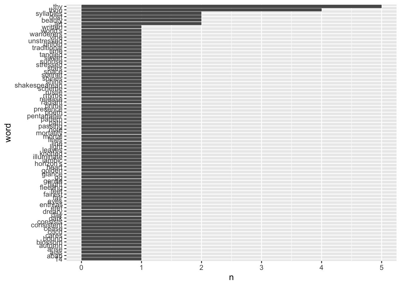
# ℹ 58 more rows

• I think I agree that’s nicer!

Let’s turn our textual word frequency list into something more graphical.

poem_tidied |>
  anti_join(stop_words) |>
  count(word) |> # Count makes a new column titled `n` with counts of each word
  mutate(word = reorder(word, n)) |> # Sorts the list of words by new column `n`
  ggplot(aes(n, word)) + # Note that this uses the `n` column made by count
  geom_col()

10.7 Sentiment Analysis

The main idea of sentiment analysis is that certain words have emotional content: positive, negative, or otherwise.

If you look over the set of words in a document and compare how frequently these different sentiments appear, you might be able to identify whether the document is tragedy or comedy – say.

As you might imagine, this isn’t the end of the story, but it works better than you might expect!

ollama run llama3 "Write a 300 word happy poem"
ollama run llama3 "Write a 300 word sad poem"

Let’s get some poems written:

happy_text <- ("Joyful moments, oh so dear,
Dance in my heart, and banish all fear.
A world of wonder, full of delight,
Where love and laughter shine with all their might.

The sun rises high in the sky,
Warming my face, and making me sigh,
With gratitude for this brand new day,
I step outside, and let joy have its way.

Birds sing sweet melodies so free,
As I walk barefoot, wild and carefree.
The wind whispers secrets in my ear,
Of possibilities, and hopes that appear.

Rays of sunshine filter through the trees,
Creating dappled patterns, full of ease.
Children's laughter echoes, pure and true,
Reminding me to let my spirit shine through.

Life is a gift, wrapped up with glee,
A chance to live, love, and be free.
So here I'll stay, in this happy place,
Where hope and joy entwine, like a tender embrace.

In this world of wonder, I am home,
Where love and light, forever roam.
I'll cherish every moment, every day,
And let my heart sing, in a happy way.

Joy is contagious, it's true,
So let's spread it far, to me and you!
Let's dance, laugh, and sing with glee,
In this world of wonder, wild and free!") |> 
   tibble(poem = _)

sad_text <- (
"In twilight's hush, where shadows play
A lonely heart beats, lost in disarray
The world outside is bright and wide
But in my soul, only darkness resides

 Memories of you linger, like a sigh
A bittersweet reminder, why I cry
The ache within me, like an open wound
Festered by the love that we left behind

Your laughter echoes, whispers in my ear
Of moments shared, and tears that we've dried here
But now you're gone, and I'm left to bear
The weight of grief, without a care

In your absence, time stands still
As I wander through the empty hills
Where our footsteps once entwined, like twine
Now lie barren, like the heart I leave behind

I search for solace, but find none
For in my dreams, you're forever gone
The stars above, a distant hum
A reminder that our love is undone

In this desolate land, I wander alone
With tears as rain, and sorrow as my throne
The winds they whisper secrets of what could've been
But like the seasons, even those whispers fade to thin

I'm left with only sorrow's bitter taste
And the ache within me, that forever will remain
In this twilight world, where shadows play
A lonely heart beats, lost in disarray"
) |> 
  tibble(poem = _)

somber_text <- (
 "In twilight's hush, where shadows play
A somber mood descends to stay
The world is gray, the heart is old
As darkness wraps its solemn hold

The wind it whispers secrets low
Of times gone by, of loved ones' woe
The trees stand tall, their branches bare
Like skeletal fingers, grasping air

The moon hides face, a ghostly glow
Casting eerie light, as all below
Is shrouded in a mournful veil
Where tears and sorrow do prevail

In this bleak landscape, I do stray
Through memories of joy that's gone astray
I search for solace, but it's hard to find
As grief and regret entwine my mind

The world is quiet, save the sighs
Of those who mourn, with tears-filled eyes
Their hearts are heavy, weighed down by pain
As they bid farewell to love in vain

In this somber hour, I do confess
A deep despair, that cannot rest
For all that's lost, for all that's past
I'm left with only memories so vast

The darkness lingers, a constant guest
A reminder of life's impermanence best
To cherish every moment we have here
And hold dear those we love, and wipe away each tear."
) |> 
    tibble(poem = _)

And let’s tidy them up and pack them together into a single table

poems <- bind_rows(
  happy_text |>
    unnest_tokens(word, poem) |>
    anti_join(stop_words) |>
    mutate(poem = "happy"),
  sad_text |>
    unnest_tokens(word, poem) |>
    anti_join(stop_words) |>
    mutate(poem = "sad"),
  somber_text |>
    unnest_tokens(word, poem) |>
    anti_join(stop_words) |>
    mutate(poem = "somber")
)
poems

# A tibble: 282 × 2
   word    poem 
   <chr>   <chr>
 1 joyful  happy
 2 moments happy
 3 dear    happy
 4 dance   happy
 5 heart   happy
 6 banish  happy
 7 fear    happy
 8 world   happy
 9 delight happy
10 love    happy
# ℹ 272 more rows

The way sentiment analysis works is that there’s a list of words, each tagged with a positive or negative “sentiment” (supposed to mean something like emotional content). There are standard lists for this… and the tidytext library has several.

For instance

bing_sentiments <- get_sentiments("bing")

Have a look! There are also c("bing","afinn","nrc","loughran") to try.

We can just inner_join these sentiments into our poems, once tidied up – adding in a column for sentiment for each word:

poems |>
  inner_join(bing_sentiments) |>
  group_by(poem) |>
  ggplot(aes(x = poem, fill = sentiment)) +
  geom_bar(position = "dodge")

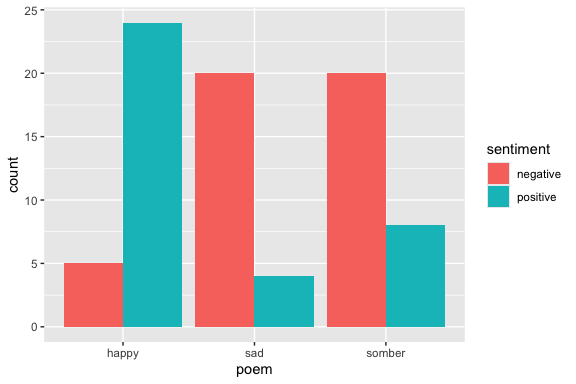
We can see that changing one word in the prompt had the effect of altering the overall word choice in the poems!

10.8 Exercise 10: Generative Models

Use the termional to get another model.

• Look over the index at https://ollama.com/library to pick a good one… but beware, the latest-and-greatest model will probably be really slow. There are little tags like these:

Tags to say how big the models are

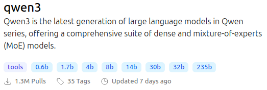
The tags on the bottom tell you the sizes of the models in billions of parameters (roughly GB of memory). For instance if you wanted the 4b model, you would use the following command:

oollama pull qwen3:4b

If all else fails, you can play with a model in the gpt2 family, since they are quite small. This one will almost certainly run for you. It even runs on my phone!

oollama pull atel3134/gpt2:124m

Since it has no prompt template, GPT2 is just for text completion. It is also comically bad at text generation, so have fun with it!

3. Play around with the model to get an idea of how it responds, including how fast it responds.

4. Look at the template for the model.

5. Try the model without the template!

6. Make a longer text using your model.

7. Produce a histogram of the top 10 most frequent words and their frequencies in the text, with stop words and any header or footer removed.

8. Use sentiment analysis to see if you can tune the sentiment by adjusting a prompt for your text.

2-Minute Neuroscience: The Neuron. 2014. https://www.youtube.com/watch?v=6qS83wD29PY.

A Grammar of Animated Graphics. n.d. Accessed May 22, 2026. https://gganimate.com/.

“albertocairo.” n.d. In albertocairo. Accessed May 22, 2026. https://www.albertocairo.com.

Alex Notov. 2025. Introduction to Claude Skills. https://platform.claude.com/cookbook/skills-notebooks-01-skills-introduction#discovering.

Anthropic. 2024. Building Effective AI Agents. https://www.anthropic.com/engineering/building-effective-agents.

Anthropic. 2025. Claude. https://claude.ai.

Anthropic. n.d.-a. “Best Practices for Claude Code.” In Claude Code Docs. Accessed April 13, 2026. https://code.claude.com/docs/en/best-practices.

Anthropic. n.d.-b. “Claude Code Overview.” In Claude Code Docs. Accessed April 16, 2026. https://code.claude.com/docs/en/overview.

Anthropic Engineering. 2025. Effective Context Engineering for AI Agents. https://www.anthropic.com/engineering/effective-context-engineering-for-ai-agents.

Anthropic Engineering. n.d.-a. “Complete Context Engineering Guide.” In Claude. Accessed April 6, 2026. https://claude.ai/public/artifacts/f498a4cc-4c45-481c-a6dd-8e1d196dadb0.

Anthropic Engineering. n.d.-b. “Prompt Engineering Overview.” In Claude API Docs. Accessed April 10, 2026. https://platform.claude.com/docs/en/build-with-claude/prompt-engineering/overview.

Anthropic Engineering. n.d.-c. “Prompting Best Practices.” In Claude API Docs. Accessed April 6, 2026. https://platform.claude.com/docs/en/build-with-claude/prompt-engineering/claude-prompting-best-practices.

API Basic Call Structures – World Bank Data Help Desk. n.d. Accessed June 1, 2026. https://datahelpdesk.worldbank.org/knowledgebase/articles/898581.

ASA, American Statistical Association. 1983. Auto Data Set from the 1983 Exposition of Statistical Graphics Technology. https://lib.stat.cmu.edu/data-expo/1983.html.

AWS. n.d. “What Is RAG? - Retrieval-Augmented Generation AI Explained - AWS.” In Amazon Web Services, Inc. Accessed June 5, 2026. https://aws.amazon.com/what-is/retrieval-augmented-generation/.

Barret, Tyson, Matt Dowle, Arun Srinivasan, et al. 2025. Data.table: Extension of ‘Data.frame‘. https://r-datatable.com.

Bartley, Kevin. 2024. “Data Statistics (2025) - How Much Data Is There in the World?” In Rivery. https://rivery.io/blog/big-data-statistics-how-much-data-is-there-in-the-world/.

Brown, Tom B., Benjamin Mann, Nick Ryder, et al. 2020. Language Models Are Few-Shot Learners. arXiv:2005.14165. arXiv. https://doi.org/10.48550/arXiv.2005.14165.

Chang, Winston. n.d. R Graphics Cookbook, 2nd Edition. Accessed May 22, 2026. https://r-graphics.org/.

Chat with Large Language Models. n.d. Accessed August 15, 2025. https://ellmer.tidyverse.org/index.html.

“Claude Code Create Custom Subagents.” n.d. In Claude Code Docs. Accessed April 19, 2026. https://code.claude.com/docs/en/sub-agents.

“Claude Code Define Your Agent.” n.d. In Claude API Docs. Accessed April 19, 2026. https://platform.claude.com/docs/en/managed-agents/agent-setup.

Codex AI Assistant for Work and Code. n.d. Accessed June 8, 2026. https://chatgpt.com/codex/.

Csardi, Garbor. 2022. Keyring: Access the System Credential Store from R. https://r-lib.github.io/keyring/index.html.

DAIR-AI. 2025. Prompt Engineering Guide. https://www.promptingguide.ai/.

Davenport, Thomas H., and D J. Patil. 2012. “Data Scientist: The Sexiest Job of the 21st Century.” Harvard Business Review October 2012: 70–76. http://hbr.org/2012/10/data-scientist-the-sexiest-job-of-the-21st-century/ar/1.

Eurostat. n.d. Data Access via API - User Guides. Accessed June 1, 2026. https://ec.europa.eu/eurostat/web/user-guides/data-browser/api-data-access.

Firke, Sam. 2024. Janitor: Simple Tools for Examining and Cleaning Dirty Data. https://sfirke.github.io/janitor/.

Fox, John, and Sanford Weisberg. 2019. An Companion to Applied Regression. Third. Sage. https://www.john-fox.ca/Companion/.

Friedman, Jerome, Trevor Hastie, and Robert Tibshirani. 2010. “Regularization Paths for Generalized Linear Models via Coordinate Descent.” Journal of Statistical Software 33 (1): 1–22. https://doi.org/10.18637/jss.v033.i01.

Gábor Csárdi. 2023. Gitcreds: Query ’Git’ Credentials from ’R’. https://gitcreds.r-lib.org/.

Ggrepel: An R Package. n.d. Accessed May 22, 2026. https://ggrepel.slowkow.com/.

Godsey, Brian. 2017. Think Like a Data Scientist. Manning.

Google. n.d. Agent Development Kit (ADK). Accessed April 19, 2026. https://adk.dev.

Grolemund, Garrett, and Hadley Wickham. 2011. “Lubridate: Dates and Times Made Easy with Lubridate.” Journal of Statistical Software 40 (3): 1–25. https://www.jstatsoft.org/v40/i03/.

Grolemund, Garrett, and Hadley Wickham. n.d. R for Data Science. https://r4ds.had.co.nz/.

Groq. n.d. API Reference - GroqDocs. Accessed June 4, 2026. https://console.groq.com/docs/api-reference#chat-create.

Hadley Wickham. 2016. Ggplot2: Elegant Graphics for Data Analysis. Springer-Verlag New York. https://ggplot2.tidyverse.org/.

Hadley Wickham, Danielle Navarro, and Thomas Lin Pedersen. n.d. Ggplot2: Elegant Graphics for Data Analysis (3e). Accessed May 22, 2026. https://ggplot2-book.org/.

Horst, Allison, Alison Presmanes Hill, and Kristen B Gorman. 2020. Palmerpenguins R Data Package. https://doi.org/10.5281/zenodo.3960218.

Ian Fellows. 2022. Wordcloud: Word Clouds. Comprehensive R Archive Network. https://doi.org/10.32614/CRAN.package.wordcloud.

Institute of Statistics (INSTAT). 2025. Statistical Database. https://databaza.instat.gov.al:8083/pxweb/en/DST/.

Institute, QLB Brain. 2017. Stunning Neuroscience Images. https://qbi.uq.edu.au/blog/2017/07/stunning-neuroscience-images.

James, Gareth, Daniela Witten, Trevor Hastie, and Robert Tibshirani. 2023. An Introduction to Statistical Learning with Applications in R. 2nd ed. Springer. https://www.statlearning.com.

Janitor: Simple Tools for Examining and Cleaning Dirty Data — Janitor-Package. n.d. Accessed May 22, 2026. https://sfirke.github.io/janitor/reference/janitor-package.html.

Kalinowski, Tomasz et al. 2022. TensorFlow for R. https://tensorflow.rstudio.com/.

Kalinowski, Tomasz, JJ Allaire, and François Chollet. 2025. Keras3: R Interface to Keras. https://keras3.posit.co/.

Kanwal, Maxinder S., Avinash S. Ramesh, and Lauren A. Huang. 2013. A Novel Pseudoderivative-Based Mutation Operator for Real-Coded Adaptive Genetic Algorithms. 2:139. F1000Research. https://doi.org/10.12688/f1000research.2-139.v2.

Kaplan, Daniel, and Randall Pruim. 2023. Ggformula: Formula Interface to the Grammar of Graphics. https://www.mosaic-web.org/ggformula/.

Karatzoglou, Alexandros, Alex Smola, Kurt Hornik, National ICT Australia (NICTA), Michael A. Maniscalco, and Choon Hui Teo. 2024. Kernlab: Kernel-Based Machine Learning Lab. https://CRAN.R-project.org/package=kernlab.

Kelechava, Brad. 2018. “The SQL Standard - ISO/IEC 9075:2023 (ANSI X3.135).” In The ANSI Blog. https://blog.ansi.org/sql-standard-iso-iec-9075-2023-ansi-x3-135/.

Keras: Deep Learning for Humans. n.d. Accessed May 28, 2026. https://keras.io/.

Khun, Max, and Julia Silge. 2023. Tidy Modeling with R. https://www.tmwr.org/.

Kingma, Diederik P., and Jimmy Ba. 2017. Adam: A Method for Stochastic Optimization. arXiv:1412.6980. arXiv. https://doi.org/10.48550/arXiv.1412.6980.

Kuhn, Max, and Hadley Wickham. 2020. Tidymodels: A Collection of Packages for Modeling and Machine Learning Using Tidyverse Principles. https://www.tidymodels.org.

Lin, Hause, and Tawab Safi. 2025. “Ollamar: An R Package for Running Large Language Models.” Journal of Open Source Software, ahead of print. https://doi.org/10.21105/joss.07211.

Luo, Junyu. 2026. Luo-Junyu/Awesome-Agent-Papers. https://github.com/luo-junyu/Awesome-Agent-Papers.

Luo, Junyu, Weizhi Zhang, Ye Yuan, et al. 2025. Large Language Model Agent: A Survey on Methodology, Applications and Challenges. arXiv:2503.21460. arXiv. https://doi.org/10.48550/arXiv.2503.21460.

Mark Lodato. n.d. A Visual Git Reference. Accessed May 30, 2026. https://marklodato.github.io/visual-git-guide/index-en.html.

Mei, Lingrui, Jiayu Yao, Yuyao Ge, et al. 2025. “A Survey of Context Engineering for Large Language Models.” In arXiv.org. https://arxiv.org/abs/2507.13334v2.

Mosaic Plots in the Ggplot2 Framework. n.d. Accessed May 22, 2026. https://haleyjeppson.github.io/ggmosaic/.

Myer, David. 2024. E1071: Misc Functions of the Department of Statistics, Probability Theory Group. https://cran.r-project.org/web/packages/e1071.

Neal Richardson, Ian Cook, Nic Crane, et al. 2026. Arrow: Integration to ’Apache’ ’Arrow’. https://github.com/apache/arrow/.

Nohe, Patrick. 2017. What Is the Dark Web? https://www.thesslstore.com/blog/what-is-the-dark-web/.

Ollama. 2025. https://ollama.com.

Ooms, Jeroen. 2014. “Jsonlite: The Jsonlite Package: A Practical and Consistent Mapping Between JSON Data and R Objects.” arXiv:1403.2805 [Stat.CO]. https://arxiv.org/abs/1403.2805.

Ooms, Jeroen. 2023. Jasonlite Vignette: Getting Started with JSON and Jsonlite. https://cran.r-project.org/web/packages/jsonlite/vignettes/json-aaquickstart.html.

Open Data Inventory—Global Index of Open Data - Open Data Inventory. n.d. Accessed May 8, 2025. https://odin.opendatawatch.com/.

OpenAI. 2025. Prompt Engineering - OpenAI API. https://platform.openai.com/docs/guides/prompt-engineering.

OpenAI. 2026. A Practical Guide to Building Agents. https://openai.com/business/guides-and-resources/a-practical-guide-to-building-ai-agents/.

OpenAI Developers. n.d. Agents SDK. Accessed April 16, 2026. https://developers.openai.com/api/docs/guides/agents.

OWASP Foundation. n.d. Least Privilege Principle. Accessed April 19, 2026. https://owasp.org/www-community/controls/Least_Privilege_Principle.

Pebesma, Edzer. 2018. “Sf: Simple Features for R: Standardized Support for Spatial Vector Data.” The R Journal 10 (1): 439–46. https://r-spatial.github.io/sf/.

Plaat, Aske, Max van Duijn, Niki van Stein, Mike Preuss, Peter van der Putten, and Kees Joost Batenburg. 2025. “Agentic Large Language Models, a Survey.” In arXiv.org. https://doi.org/10.1613/jair.1.18675.

Plotly r Graphing Library in R. n.d. Accessed May 23, 2026. https://plotly.com/r/.

Posit. 2025a. Posit Cheatsheets. https://posit.co/resources/cheatsheets/.

Posit. 2025b. Positron. https://positron.posit.co/.

Posit. 2025c. “RStudio IDE User Guide.” In RStudio User Guide. https://docs.posit.co/ide/user/.

Posit. 2026. “Quarto Guide.” In Quarto. https://quarto.org/docs/guide/.

Positron. n.d.-a. “Guide for Positron Assistant.” In Positron. Accessed April 18, 2026. https://positron.posit.co/assistant.html.

Positron. n.d.-b. “Positron Assistant Getting Started.” In Positron. Accessed April 18, 2026. https://positron.posit.co/assistant-getting-started.html.

Quarto. 2025. Posit.co. https://quarto.org/.

Rashida048. 2020. Machine Learning: Gradient Descent Concept – Regenerative. https://regenerativetoday.com/machine-learning-gradient-descent-concept/.

Robinson, Julia Silge and David. n.d. Text Mining with R. Accessed April 12, 2020. https://www.tidytextmining.com/.

Ruman. 2023. “Convex Vs. Non-Convex Functions: Why It Matters in Optimization for Machine Learning.” In Medium. https://rumn.medium.com/convex-vs-non-convex-functions-why-it-matters-in-optimization-for-machine-learning-39cd9427dfcc.

Sahoo, Pranab, Ayush Kumar Singh, Sriparna Saha, Vinija Jain, Samrat Mondal, and Aman Chadha. 2024. “A Systematic Survey of Prompt Engineering in Large Language Models: Techniques and Applications.” In arXiv.org. https://arxiv.org/abs/2402.07927v2.

Silge, Julia, and David Robinson. 2023. Tidytext: Text Mining Using Tidy Tools. https://juliasilge.github.io/tidytext/.

Silge, Julia, and David Robinson. 2025. Tidytext: Text Mining with R. O’Reilly Media, Inc. https://www.tidytextmining.com/.

Simple Tools for Examining and Cleaning Dirty Data. n.d. Accessed May 22, 2026. https://sfirke.github.io/janitor/index.html.

Sjoberg, Daniel D., Karissa Whiting, Michael Curry, Jessica A. Lavery, and Joseph Lamarange. 2021. “Reproducible Summary Tables with the Gtsummary Package.” The R Journal 13 (1): 570–80. https://doi.org/10.32614/RJ-2021-053.

Stryker, Ivan Belcic, Cole. 2024. What Is Data Engineering? IBM. https://www.ibm.com/think/topics/data-engineering.

Takeda, Hajime. 2026. “How to Build a Production-Ready Claude Code Skill.” In Towards Data Science. https://towardsdatascience.com/how-to-build-a-production-ready-claude-code-skill/.

Team, R Core. 2018. R: A Language and Environment for Statistical Computing. R Foundation for Statistical Computing. https://www.R-project.org/.

“TensorFlow.” n.d. In TensorFlow. Accessed May 28, 2026. https://www.tensorflow.org/.

The Composer of Plots. n.d. Accessed May 22, 2026. https://patchwork.data-imaginist.com/.

“The Visual Display of Quantitative Information.” n.d. In Edward Tufte. Accessed May 22, 2026. https://www.edwardtufte.com/book/the-visual-display-of-quantitative-information/.

Ushey, Kevin, JJ Allaire, and Yuan Tang. 2023. Reticulate: R Interface to Python. https://rstudio.github.io/reticulate/.

van Rossum, Guido. 2025. Python. https://www.python.org/.

Vaswani, Ashish, Noam Shazeer, Niki Parmar, et al. 2023. Attention Is All You Need. arXiv:1706.03762. arXiv. https://doi.org/10.48550/arXiv.1706.03762.

VoltAgent/Awesome-Claude-Code-Subagents. 2026. VoltAgent. https://github.com/VoltAgent/awesome-claude-code-subagents.

Waring, Elin, Michael Quinn, Amelia McNamara, Eduardo Arino d la RUbia, Shu Hao, and Shannon Ellis. 2025. Skimr: Compact and Flexible Summaries of Data. https://docs.ropensci.org/skimr/.

Weng, Lilian. 2023. Prompt Engineering. https://lilianweng.github.io/posts/2023-03-15-prompt-engineering/.

Wickham, Hadley. 2010. “A Layered Grammar of Graphics.” Journal of Computational and Graphical Statistics 19 (1): 3–28. https://doi.org/10.1198/jcgs.2009.07098.

Wickham, Hadley. 2016. Ggplot2: Elegant Graphics for Data Analysis. Springer-Verlag New York. https://ggplot2.tidyverse.org/.

Wickham, Hadley. 2023a. Forcats: Tools for Working with Categorical Variables (Factors). https://forcats.tidyverse.org/.

Wickham, Hadley. 2023b. Httr2: Perform HTTP Requests and Process the Responses. https://httr2.r-lib.org/.

Wickham, Hadley. 2023c. Modelr: Modelling Functions That Work with the Pipe. https://modelr.tidyverse.org/.

Wickham, Hadley. 2023d. Stringr: Simple, Consistent Wrappers for Common String Operations. https://stringr.tidyverse.org/.

Wickham, Hadley, Mara Averick, Jennifer Bryan, et al. 2019. “Welcome to the Tidyverse.” Journal of Open Source Software, no. 43: 1686. https://doi.org/10.21105/joss.01686.

Wickham, Hadley, and Jennifer Bryan. 2023. Readxl: Read Excel Files. https://readxl.tidyverse.org.

Wickham, Hadley, Mine Cetinkaya-Rundel, and Garrett Grolemund. 2023. R for Data Science (2e). O’Reilly Media, Inc. https://r4ds.hadley.nz/.

Wickham, Hadley, Romain Francois, Lionel Henry, Kirill Muller, and Davis Vaughan. 2023. Dplyr: A Grammar of Data Manipulation. https://dplyr.tidyverse.org.

Wickham, Hadley, Jim Hester, and Jennifer Bryan. 2024. Readr: Read Rectangular Text Data. https://readr.tidyverse.org/.

Wickham, Hadley, Davis Vaughan, and Maximilian Girlich. 2023. Tidyr: Tidy Messy Data. https://tidyr.tidyverse.org.

Wikipedia. 2025. “Data Science.” In Wikipedia. https://en.wikipedia.org/wiki/Data_science.

World Bank. n.d.-a. About the Indicators API Documentation. Accessed June 1, 2026. https://datahelpdesk.worldbank.org/knowledgebase/articles/889392-about-the-indicators-api-documentation.

World Bank. n.d.-b. Indicator API Queries. Accessed June 1, 2026. https://datahelpdesk.worldbank.org/knowledgebase/articles/898599-indicator-api-queries%3E.