https://posit.cloud/spaces/650740/join?access_code=nPYTxhqfZdAf8z1dwhQZuanYuJK34OocIoy5Zb–
1 Data Science (DS), a DS Life Cycle, and Getting Data
Keywords
data science, life cycle, Posit Cloud, Quarto, RStudio, readr
1.1 Course Introduction
1.1.1 Purpose of this Course
- Introduce a wide variety of data science methods across the data science life cycle
- Build foundational knowledge of and experience in basic data science methods and capabilities.
- Introduce concepts and methods for working with machine learning and Artificial Intelligence (AI) systems
1.1.2 Description
- This course uses multiple modules to introduce data science methods using the R programming language and the set of R packages known as the tidyverse.
- Each module discusses specific data science methods followed by practical exercises to gain hands-on-keyboard experience in using these methods to work with data and generate results.
1.1.3 Learning Outcomes
After successful completion of this course, you should be able to …
- Identify appropriate data science methods to address common issues in working with data.
- Use statistical programming capabilities to access data, conduct exploratory analysis of data sets, develop and tune basic models to produce develop insights from the data.
- Describe and apply concepts, methods and tools associated with AI systems
1.1.4 Course References
- R Programming Language (Team 2018)
- R for Data Science (2e) (Wickham, Cetinkaya-Rundel, et al. 2023)
- RStudio User Guide (Posit 2025c)
- Quarto open-source scientific and technical publishing system (Quarto 2025)
- {tidyverse} package (Wickham et al. 2019)
- Posit Cheat Sheets (Posit 2025a)
1.2 Module Introduction
This Module will address the following topics
- What is Data Science?
- A Data Science Life Cycle.
- Introduction to R and RStudio in Posit Connect
- Sources of data to include Open data.
- Different types of data formats: .csv files, excel files, urls, compressed data, Arrow-Parquet
- Rectangular data, vectors and data frames in R
- Methods for getting rectangular data from other sources or files into R data frames.
- Viewing data and getting summary statistics about data in R data frames.
Learning Outcomes
- Access Posit Cloud and RStudio
- Explain different sources of data
- Explain different types of data formats
- Load data from open data sources into R
- View data and get summary statistics about data in R data frames
Module References
1.3 What is Data Science?
Wikipedia has a long history of the words Data Science but starts with the definition:
“Data science is an interdisciplinary academic field that uses statistics, scientific computing, scientific methods, processing, scientific visualization, algorithms and systems to extract or extrapolate knowledge from potentially noisy, structured, or unstructured data.”(Wikipedia 2025)
In October 2012, the Harvard Business Review’s article Data Scientist: The Sexiest Job of the 21st Century”identified Data Scientists as “people who can coax treasure out of messy, unstructured data.” (Davenport and Patil 2012)
There are many other definitions but most include some aspect of “interdisciplinary” as seen in Figure 1.1 where data science sits in the intersection of computing, statistics, and expertise about a domain such as business, or medicine.
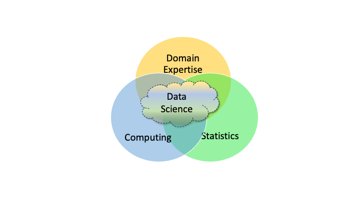
Figure 1.1 provides an overview but a more detailed taxonomy of a Data Science “Body of Knowledge” could include the following categories as additions to the figure.
- Foundations: Statistics, Mathematics, Computing, Data Life Cycle, Data Science Life Cycle, Communications
- Modeling and Analysis: Machine Learning, AI, Operations Research, Geospatial
- Collaboration: Individual, Team, Technical
- Responsible Data Science: Legal Considerations, Ethical Considerations, Frameworks for Fairness, Bias Identification and Mitigation, Trustworthy AI/ML
- Interactive Solutions: Dashboards; Web-Applications, Web Development
- Big Data: Large Scale Computing
- Deployment: Sharing, Hosting, Operations, Continuous Integration/Continuous Deployment
Yet, no two Data Scientists are the same. The cloud in an expanded version of Figure 1.1 grows and shifts for each individual as they focus on the kinds of problems they like to solved.
- That is why Data Science work is almost always a “team sport” as no one knows everything.
In closing:
A competent data scientist is someone who knows how to get, manipulate, visualize, and analyze data and, as needed, build and deploy a useful model for answering a question.
A happy data scientist is a someone who thrives when combining their competence with curiosity, creativity, and persistence to create solutions in areas of life in which they are passionate.
Data science emerged this century by building on decades of prior work in mathematics, statistics, and operations research and the explosive growth of computing, storage capacity, and network connectivity.
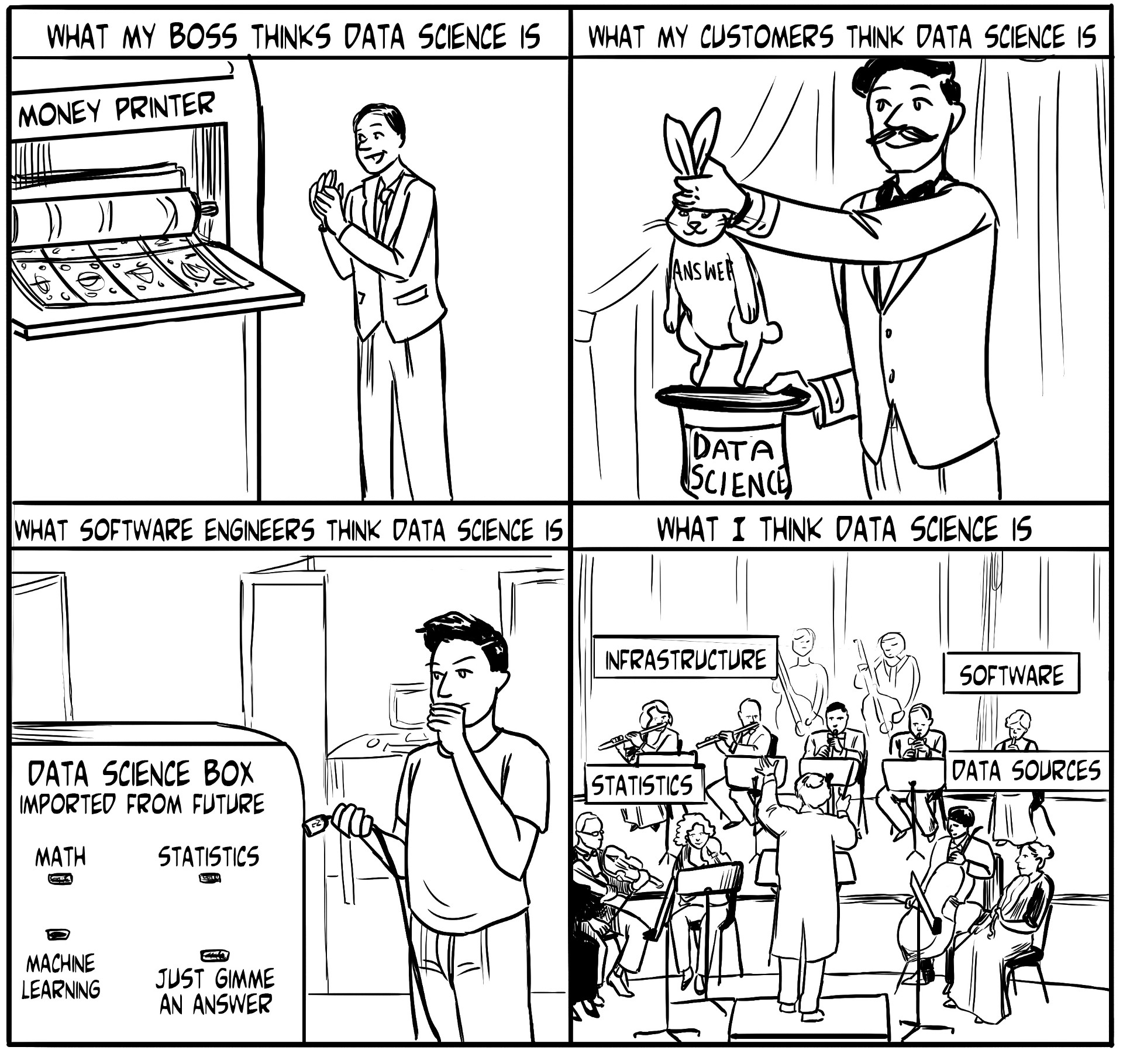
However, ask four people “What is data science?”; you might get four different answers as in Figure 1.2.
1.4 Artifical Intelligence and Machine Learning
You will hear a lot of terms in discussions about Artificial Intelligence (AI) and Machine Learning (ML).
For the purposes of this course, the Venn diagram in Figure 1.3 provides some context.
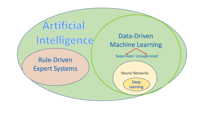
AI can be considered an umbrella category which has been around for decades. Under that umbrella are
Rule-driven expert systems, where human subject matter experts in different domains tried to encode their expertise or knowledge into “rules” to guide machine decision making with deterministic logic or inference systems.
Data-driven Machine Learning systems “learn from the data” and possibly some constraints.
Supervised learning uses labeled data with a known Response or target the ML system is trying to match.
Unsupervised learning uses unlabeled data where there no known Response and the ML system is trying to find “patterns” in the data.
There are also hybrid systems that combine features of both.
Neural Networks are a specific kind of ML modeling approach where the model has “layers” of multiple interconnected “neurons.” Each neuron performs a non-linear transformation of its input to produce an output, allowing the network to approximate complex functions.
Deep Learning is a sub field Neural Networks were there can be many layers and many, many neurons in each layer.
If you think of each neuron as having two parameters (weight and bias) and then you hear about recent models with 70B parameters, you get a sense for how large and complex these models can be.
1.5 A Data Science Life Cycle
Responsible Data Science depends upon following a repeatable process or life cycle for analysis and solution development.
There are many different life cycles and frameworks in the community. Some are tailored to one aspect of data science. Others attempt to include all aspects of data science in a single framework.
This course will use the following life cycle as a frame of reference given its focus on answering a question of interest.
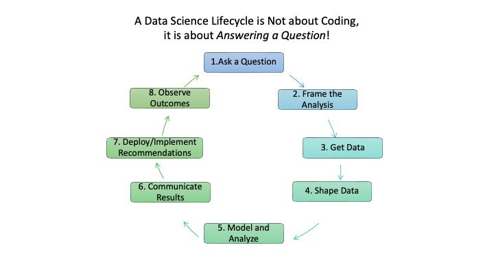
- Figure 1.4 portrays eight steps for a Data Science life cycle that start with someone asking a question and end with observing the outcomes of the solution.
- Some might be tempted to stop at an earlier step, but a data scientist knows that every analysis and solution is based on assumptions, explicit and implicit.
- Observing outcomes is a responsible approach to validating if assumptions were valid or responsible.
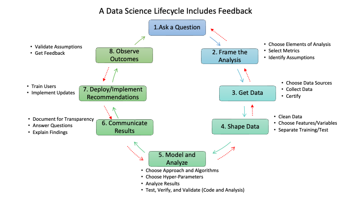
- Figure 1.5 provides additional details on the types of activities that can occur within each step.
- It also highlights that while Figure 1.4 shows a nice, circular process that is always making progress, responsible data science often takes one step forward and then two steps backwards.
- Feedback from the activities at a step might indicate one should back up and repeat an earlier step.
- As an example, if modeling and analysis shows the data is not as robust as desired or shows sampling bias that will render the results less useful for the question, one may need to back up to step 3 to get more data or even step 1 to get guidance on reframing the question of interest.
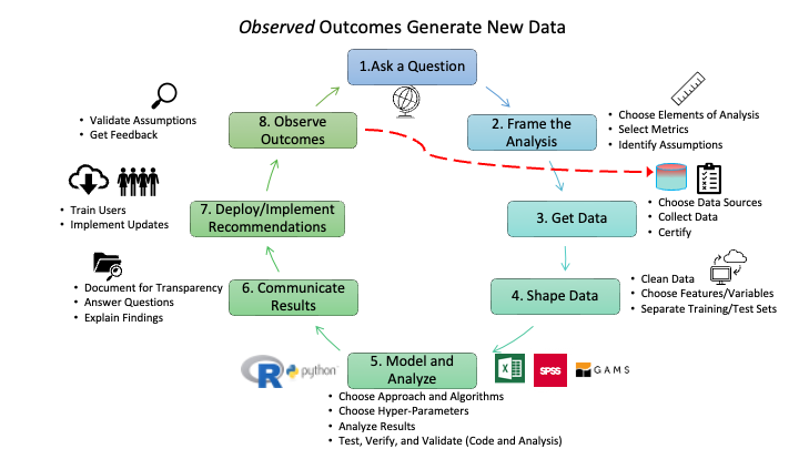
- As implementation occurs, it will usually generate new data that could support future analysis.
- Responsible data science will use this new data to assess assumptions made in building the solutions and whether there is disparate impact on the populations affected by the implementation.
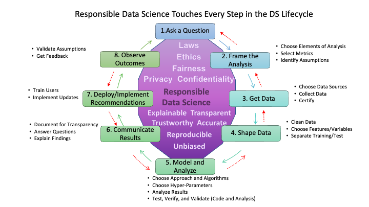
- Figure 1.7 shows that responsible data science is not a single step in the life cycle but underlies activities at each step in the life cycle.
- The top of the figure identifies several considerations for shaping the analysis or solution at each step to ensure the analysis or solution complies with laws and ethical guidelines while minimizing risks to fairness, privacy, and confidentiality of data and people.
- The bottom of the figure identifies attributes for the activities at each step to ensure the work aligns with principles for responsible data science.
- We will address aspects of responsible data science throughout the course.
1.6 Tools for Data Science
Data Scientists typically use three kinds of tools:
- Programming Languages: for writing code to get, manipulate, and analyze/visualize data and then use the data to build models, test hypotheses, and communicate their results.
- Integrated Development Environments: Tools for working with programming languages with built in capabilities for coding, debugging, version control, and now many have built in AI-supported copilots or agent support.
- “Notebooks” and Scripts: Documents designed for working with code to help document the work, document the code, to enable reuse, sharing, collaboration and reproducibility.
- Notebooks are documents designed to enable “literate programming” that involves integrating code and text about the work, the code and/or the results. Scripts are code-centric files for organizing and documenting code for efficient programming and usage.
1.6.1 Programming Languages
Many data scientists are “tri-lingual” meaning they can code in three languages:
- The statistical programming language R

- The general programming language Python
 , and,
 - The relational database-centric language Structured Query Language more commonly known as SQL.
However, many also know other languages such as Julia or STATA and most have familiarity with “languages” such as Regular Expressions(regex) for manipulating text, HTML for working with web sites and web pages, and CSS for working with web page element attributes such as id or class structures.
1.6.1.1 Why is R so popular?
- It’s great for practitioners doing rapid interactive statistical analysis.
- It’s free and open source. You will always have access to R.
- It’s widely-used with a lot of community support.
- It’s relatively easy (especially graphics and data wrangling) as its “evolution” was driven by statisticians for local utility.
- It enables reproducible research and analysis.
1.6.1.2 R is a Statistical Programming Language
- R was specifically designed for statistical analysis and presentation.
- Special features make it “quirky” but effective for our purposes.
- It’s a vector language, has low-level support for missing values, is function-oriented, has few but powerful built-in data structures
- You write R code using text to describe what you want R to do
- You tell R when to do something
- Immediately for interactive analysis.
- On demand when you “run” one or more lines of code at once.
- R can support all data analysis tasks (and much more!).
- R is built around the idea of packages: like apps
- Packages are sets of functions designed to work together to accomplish a specific set of tasks
- There are over 15K packages on the central repository covering all aspects of data science.
1.6.1.3 Different Flavors of R Work Together
There are three main flavors of R: Base R (Team 2018), the tidyverse (Wickham et al. 2019), and data.table (Barret et al. 2025).
- Base R is the foundation: it has broad functionality but is often not as intuitive or consistent as the tidyverse or data.table.
- The tidyverse is a curated set of packages on top of Base R designed around a common approach and consistent syntax for doing interactive statistical analysis in a way that is more convenient and easier to learn for many tasks - think of functions as verbs and the data as nouns.
- data.table is a package designed around being very fast when manipulating very large data sets.
- All three flavors work well together
1.6.1.4 What about Python?
Python is also a great language for data science.
- As a more general computer language (over 627K packages), it can be used for developing broader applications.
- Some prefer it because its design and syntax is more like a standard computer language.
- It is especially strong when working with AI/ML models that are part of large systems.
Most data scientists know R and Python to some level of expertise.
- They choose the tool based on the use case, their collaborators, and which has the better packages for their needs.
- Since R and Python can work well together, you can choose the best fit for different parts of your analysis.
1.6.2 Integrated Development Environments (IDEs)
Billions of lines of code have been written in basic text editors as most code is just text.
IDEs evolved as Graphical User Interfaces were developed starting in the 1980s.
They can help make developers more efficient as they provide:
- Help for the language
- Error-checking
- Debugging Support
- Version Control Support
- Support for Connections to Data Sources
- Support for AI copilots or Agents
Two common IDEs in Data Science are RStudio (R-oriented) and Jupyter Notebooks (Python-oriented)
- Both of these have evolved to support other languages as well.
There are also specialized IDEs for other languages such as DBeaver for SQL
Visual Studio Code is a very popular general purpose, multi-language IDE built and licensed by Microsoft built on the open source Visual Studio Code - Open Source (“Code - OSS”)
Positron is a new multi-language IDE from Posit (the makers of RStudio) that is built on top of the same OSS foundation as VSCode but it is designed specifically for data science and statistical programming.
1.6.3 Using “Notebooks” for Literate Programming
Literate Programming is a term popularized by Turing award winning Computer Scientist Donald Knuth.
One of his many quotes is:
When you write a program, think of it primarily as a work of literature. You’re trying to write something that human beings are going to read. Don’t think of it primarily as something a computer is going to follow. The more effective you are at making your program readable, the more effective it’s going to be: You’ll understand it today, you’ll understand it next week, and your successors who are going to maintain and modify it will understand it.
Literate programming is characterized by the use of “notebooks” to support inter-active coding.
- Each notebook has one or more text blocks of discussion, then the a code block or chunk, then a block of results for the code such as images, and then more text discussion about the results of the code.
- This is different than the usual script files of just code (with comments) that is designed to be run in sequence.
- Many scripts are first developed in a notebook and then converted to scripts once they are mature.
With interactive programming, data scientists can document their ideas and code as they go along. This supports clear understanding about the code and helps create reproducible results.
1.6.3.1 Quarto
Quarto is an open-source scientific and technical publishing system from Posit.co that supports literate programming via notebooks.
Quarto users create plain-text notebook (.qmd) files using YAML and R Markdown tags.
- Being text based makes it easy to work with version control systems and share code.
Quarto is designed as a Command Line Interface in the Terminal window but is also integrated into RStudio and works in JupyterLab, Positron, VSCode, and Text Editors.
- Quarto users can convert (render) their plain text notebook files into multiple formats.
- One document can be used to create reports, journal articles, presentations, web content,… in HTML, PDF, Word, PowerPoint, … All Formats.
- Quarto supports using multiple “themes” with options for customized CSS/SCSS, or \(\LaTeX\).
- Quarto supports math with MathJax (including AMSmath).
Quarto has extensive on-line documentation, an active community, and numerous videos and blogs.
- The RStudio Hello, Quarto Tutorial or Authoring: R Markdown Basics can help you get started.
- Additional tutorials and sections under Authoring describe many new features of Quarto.
Now that we kmnow the tools we will use, R, RSTudio and Quarto, let’s look at where we can get the some data.
- We will use data sets that come with R and data we can download from the internet, known as Open data.
1.7 Open Data
With over 181 Zetabytes (1ZB = 1M Petabytes) as of 12/24, there is a lot of data in the world.
If you think of the web as an iceberg, as in Figure 1.8, only the 4% above the water level is freely accessible “Open data”.
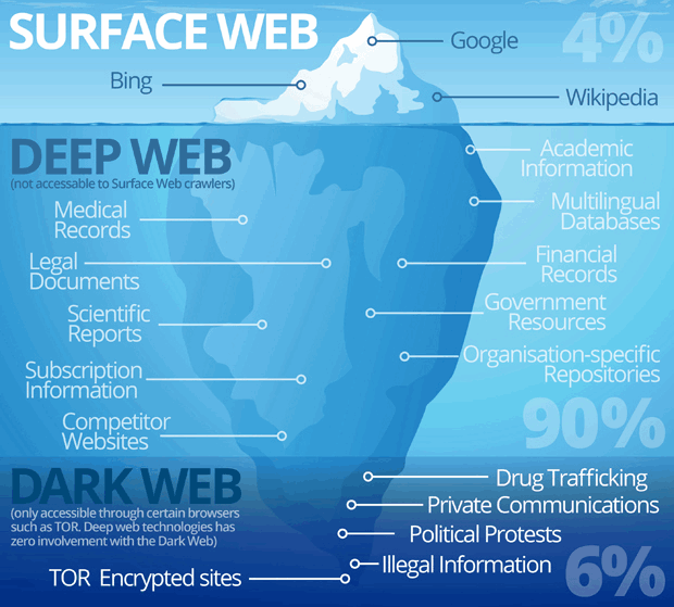
- Above the water is known as the “surface web”, where web-crawlers, search engines, and you roam freely.
- There is much more data below the surface - in the deep web.
- This data is protected behind firewalls or application programming interfaces (API) where general search engines (or you) can’t access it without additional steps to establish your identity.
- This includes business data, educational data, health data, … any data that the owner wants to or is required to protect.
- The bottom 6%, below the deep web, is the “Dark Web”, where accessing sites require special browsers and routers.
1.7.1 Sources of Open Data
Many Countries Have Open Data Laws that require unclassified or protected government data be made open for public use.
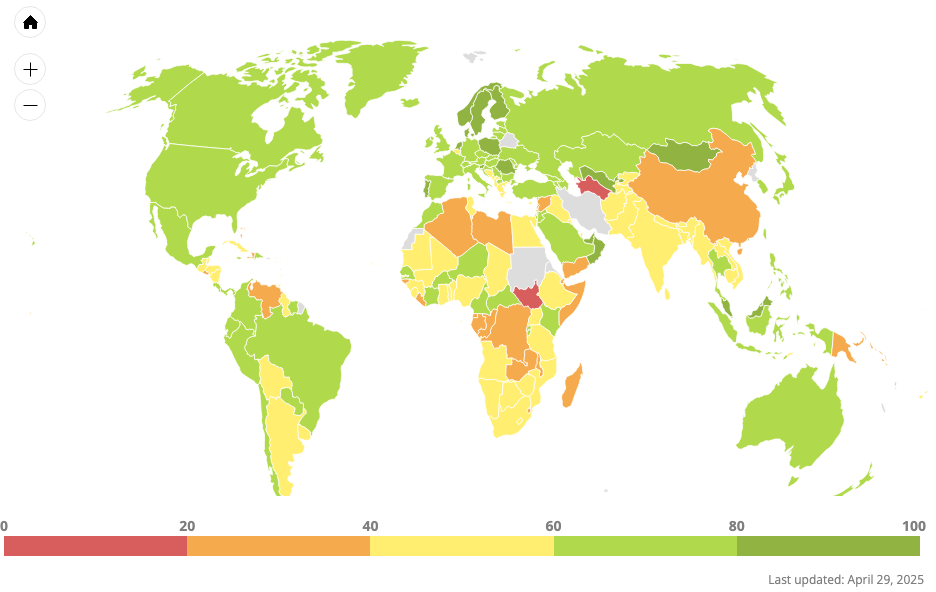
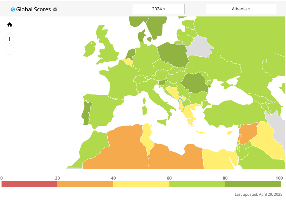
Open Data Watch (ODW) is an international, non-profit organization of data experts dedicated to transforming how official statistics are produced, managed, and used.
- The Open Data Watch (ODW) Open Data Inventory (ODIN) assesses the coverage and openness of official statistics to identify gaps, promote open data policies, improve access, and encourage dialogue between national statistical offices (NSOs) and data users.
Sources of global open data.
- United Nations
- World Bank
- International Monetary Fund
- Organisation for Economic Co-operation and Development (OECD)
- Open Data Portal Europe
Many countries have their own Open Data portals.
- Albanian National Institute of Statistics (INSTAT) (Institute of Statistics (INSTAT) 2025) has lots of data.
- Republic of Albania Open Data Site has some data.
- Republic of Northern Macedonia
- United States
Organizations Sponsor Open Data Sites (some charge a fee)
Bottom Line: > Data, Data Everywhere with Billions and Billions of Bytes to Think
with apologies to English poet Samuel Taylor Coleridge
1.7.2 Open Data Formats
Open a browser and go to the Opendata.gov.al, (select English as the language?) and click on Economy and Finance.
Your browser could look something like Figure 1.9.
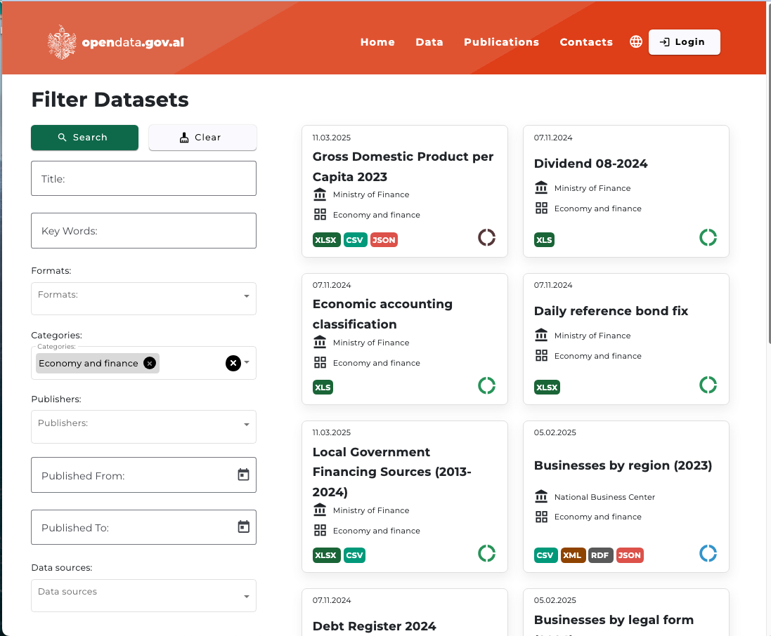
You can see at the bottom of the entries for each data set are a set of icons that indicate the formats you can download.
Common types include:
- XLSX: the standard for Microsoft Excel™ workbook files
- CSV: Comma Separated Values
- JSON: JavaScript Object Notation which is an open format composed of Key: value pairs. It is a data format and not part of the Javascript language.
- XML eXtended Markup Language: A structured markup language using nested tags and attributes to represent hierarchical data with explicit metadata and validation rules.
- RDF Resource Description Framework: RDF extends the linking structure of the Web to use URIs to name the relationship between things as well as the two ends of the link (this is usually referred to as a “triple”). Using this simple model, it allows structured and semi-structured data to be mixed, exposed, and shared across different applications.
Paste into your browser the link https://opendata.gov.al/datasets-list/toka_per_qiradhenie which should take you to a page for the Land for Rent under Agriculture, Fisheries, forestry and food category.
- You should see a page like in Figure 1.10.
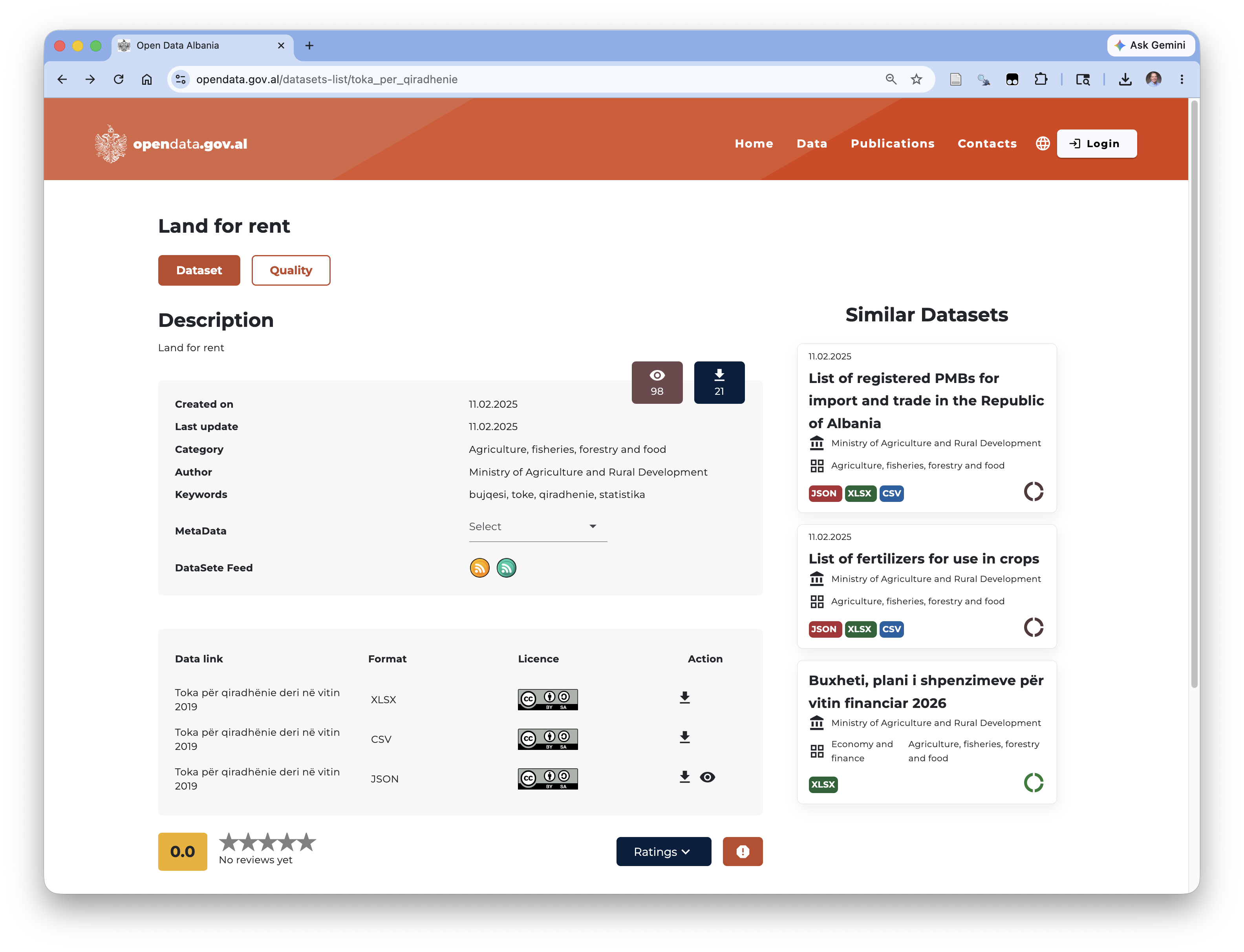
Action which indicate you can download the format.
If you click the first two arrows you will download a .CSV file and a .xlsx file to your computer’s default downloads location for your browser.
- If you open the .xlsx file. it should look like Figure 1.11.
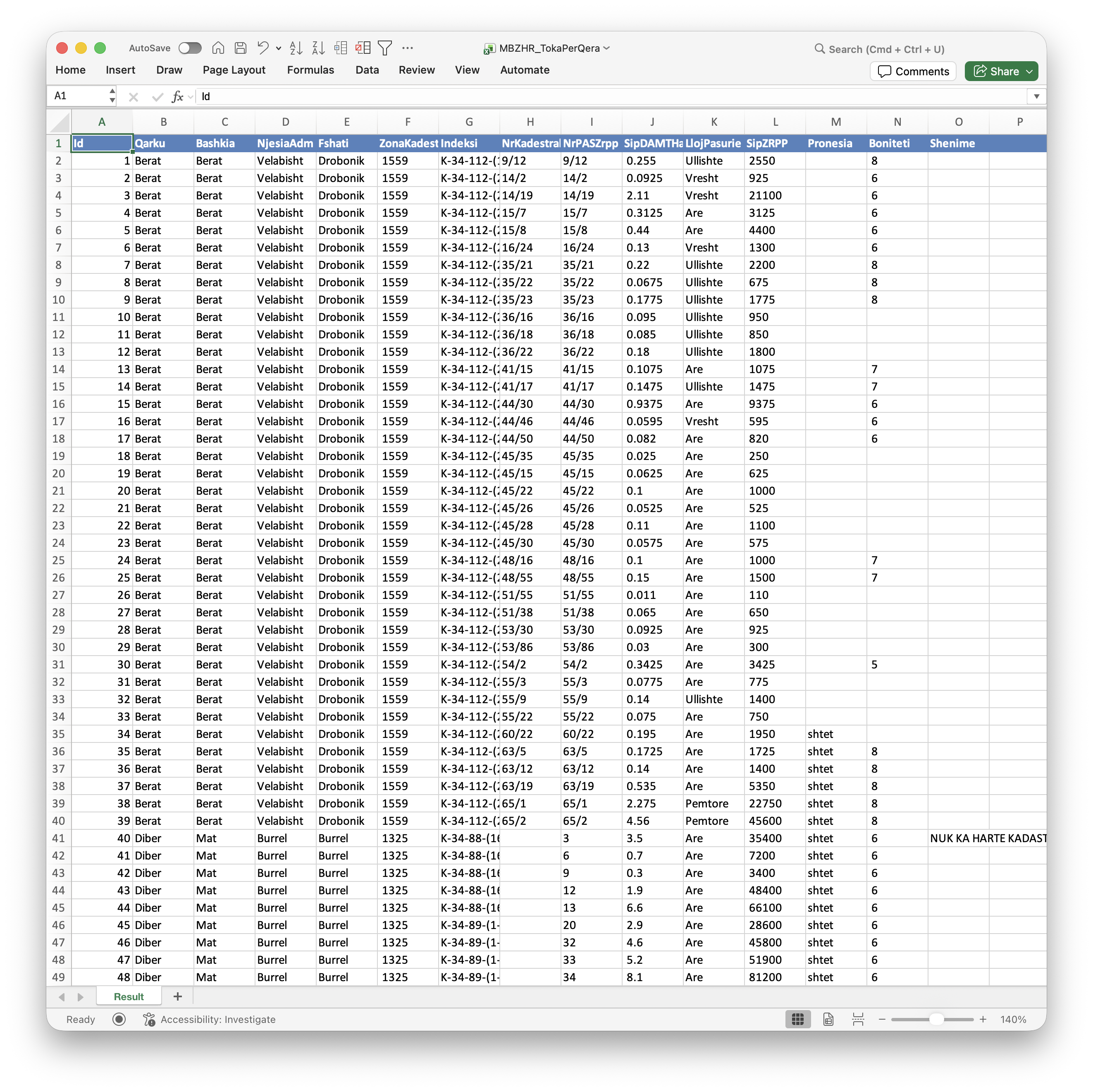
- If you open the .csv file with the default, it should look just Figure 1.11 as many computers default to using a spreadsheet application to open a .csv file. However, it does not. It looks like Figure 1.12.
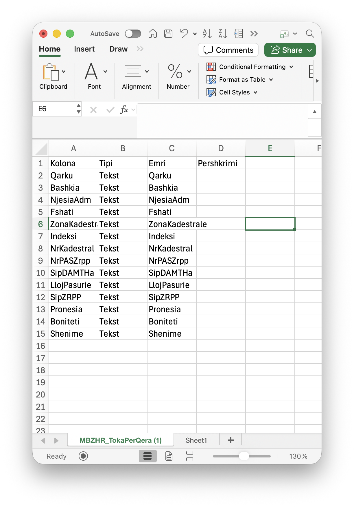
This appears to be more like the data dictionary (meta-data) for the dataset instead of the actual data.
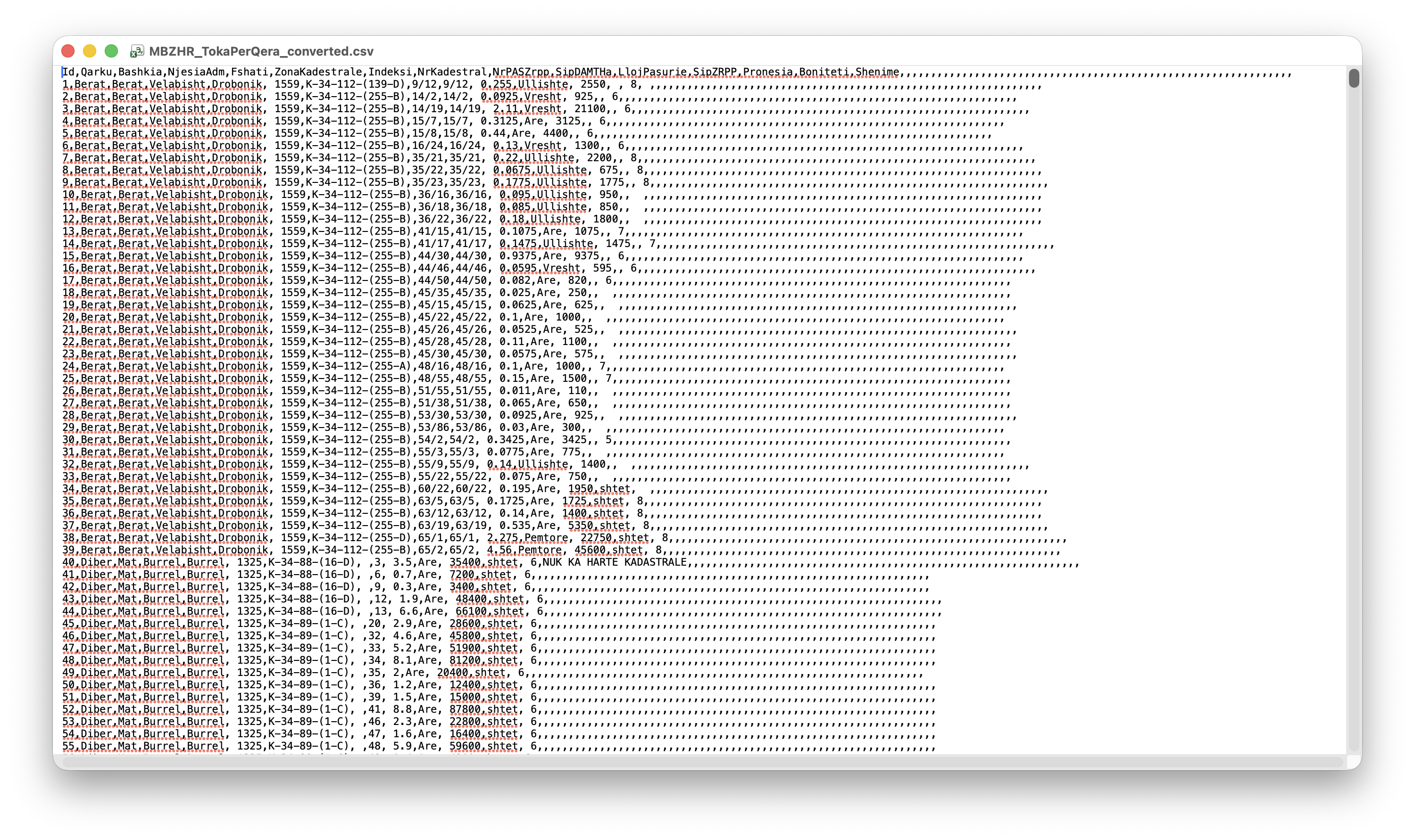
If you save the Excel File in CSV format and open it with a text editor, you will get what the data actually looks like as in Figure 1.13
- Notice the commas “,” separating each value.
- Also note that Excel stuck on many additional “ghost” columns that are empty. These should get handled when cleaning the data.
- However, if you click on the JSON download arrow, it could open in your browser to look like Figure 1.14.
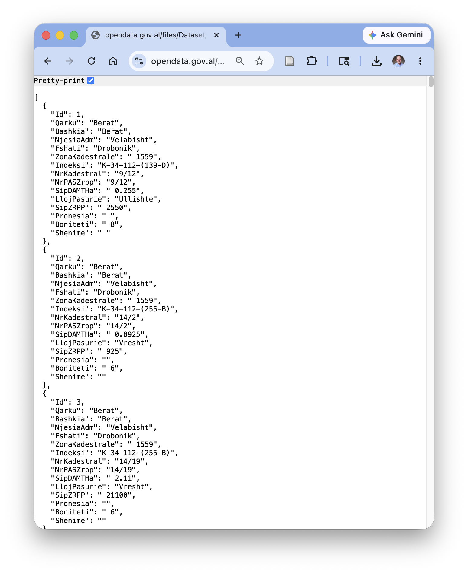
- Note the key-value pairs for each observation.
- If you click on the browser menu to save the page, then it should download the file.
These are three common formats for open data.
- The XLSX and CSV formats work well with “rectangular” data or data where every row has the same number of columns so it fills a table nicely.
- Think of the rows as the records or observations of some entity and each column is an attribute or variable of the entity and the intersection is the value for that variable for a given observation.
- A drawback of rectangular data is that complex data may require adding a lot of redundant data in the table to capture all the relationships, increasing the file size.
- JSON can support rectangular data quite well, but it is much more flexible. By nesting the key value pairs it can support complex data quite efficiently.
- If a file is more than a few MB, many sources may compress any of these formats using a ZIP format to reduce the time and space to download.
R and Python both work well with all three types including their compressed versions.
1.7.3 Newer Data Storage and Exchange Formats
There are newer formats for storing and exchanging data that are gaining in popularity, especially for very large and/or distributed data sets.
- They often focus on working with data relationships as columns instead of rows as most data science work focuses on the variables. See What is a Columnar Database.
- In addition to the data values, many of these allow for the storage of meta-data as well.
- Columnar storage format (data stored column-wise)
- Optimized for querying, compression, and scanning large data sets
- Ideal for big data workflows (e.g., with the R Arrow package, Spark, Hive, Python Pandas, or new DuckDB data bases)
Use when: You want fast reads/writes on large tabular data sets, especially with repeated column access.
- In-memory data format for high-performance analytics
- Basis for Feather, and used by Parquet under the hood
- Enables zero-copy reads across systems (e.g., from Python to R to C++)
Use when: You need fast in-memory analytics or to move data between tools without conversion.
- Columnar binary format based on Apache Arrow
- Designed for speed and interoperability between R and Python
- Often used in data science pipelines for medium-sized data sets
- Smaller and faster than CSV for tabular data
Use when: You want fast, language-interoperable serialization for in-memory tables.
- ORC (Optimized Row Columnar) - for Really big data
- Similar to Parquet, but more common in Hadoop/Hive environments
- Great for complex nested data and compression
- Often used in enterprise-scale data lakes
Use when: You’re working in a Hive or Hadoop ecosystem.
Important
For simplicity, we will work with CSV files for most of this course.
Now that we have sources for data, let’s connect to Posit Cloud to access RStudio where we can gtet data and begin working with it.
1.8 Posit Cloud
1.8.1 Posit and Posit Cloud
Posit.co is a US-based Public Benefit Corporation focused on creating open-source software for data science, scientific research, and technical communication.
- They evolved out of the RStudio organization as they expanded their focus to support R and Python.
- Their open source (free) software includes:
- The RStudio Integrated Development Environment (IDE)
- The Tidyverse set of R packages
- Quarto
- R Shiny and Python Shiny
- The RStudio Integrated Development Environment (IDE)
- Their product services include:
- Posit Connect
- Posit Cloud
- shinyapps.io - for hosting shiny apps.
Data scientists typically install all the open source software on their local computer.
- If you want to do that, see Installing Languages and IDEs for some ideas.
However, for most of this course, we will be using Posit Cloud so you do not need to install any software for now.
- Posit Cloud is a cloud-based environment where you use browser-based access to R, the RStudio IDE, and your data to support data science work.
- This course is structured so you can establish a free account to accomplish all of the exercises.
1.8.2 Accessing the Posit Cloud Course Workspace
1.8.2.1 Get a Posit Cloud Free Account and Access Posit CLoud
Sign up for the Free plan (not the student plan) by going to Plans & Pricing Free.
- You should see a screen like Figure 1.15.
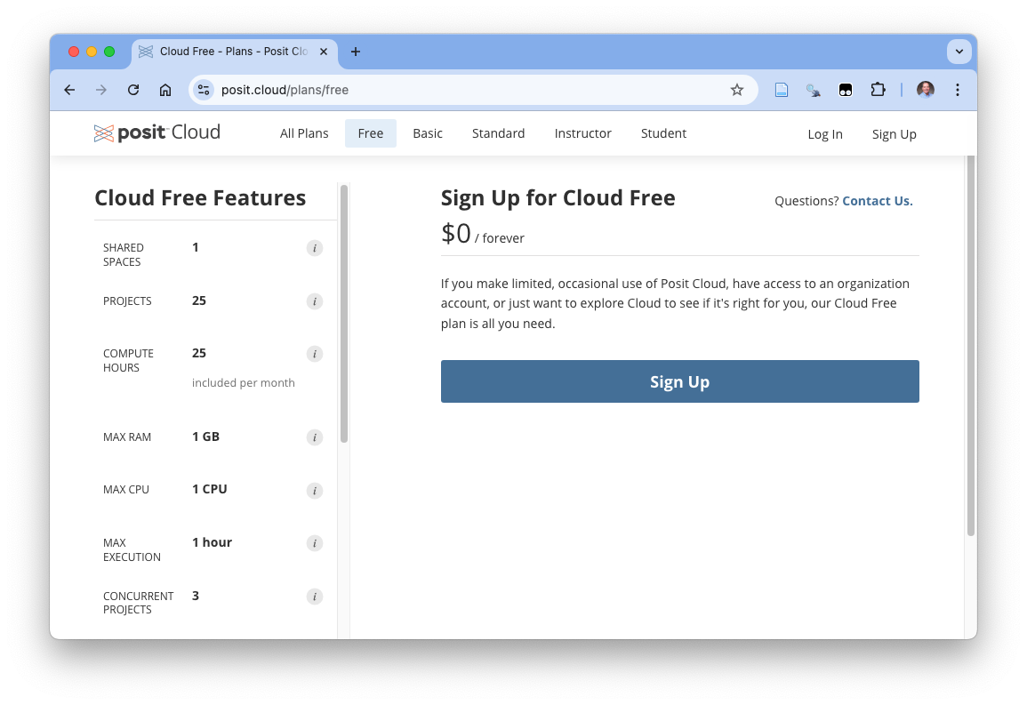
- Click on
Sign Up. This will take you to a page to fill in your account information. - Fill out the information with your email, new password, and name, and click on
Sign Up. - This will open a verification page.
- Go to your email account and look for the verification email.Click on the verification link in the email.
- You should now see a page with your new Posit Cloud workspace similar to Figure 1.16.
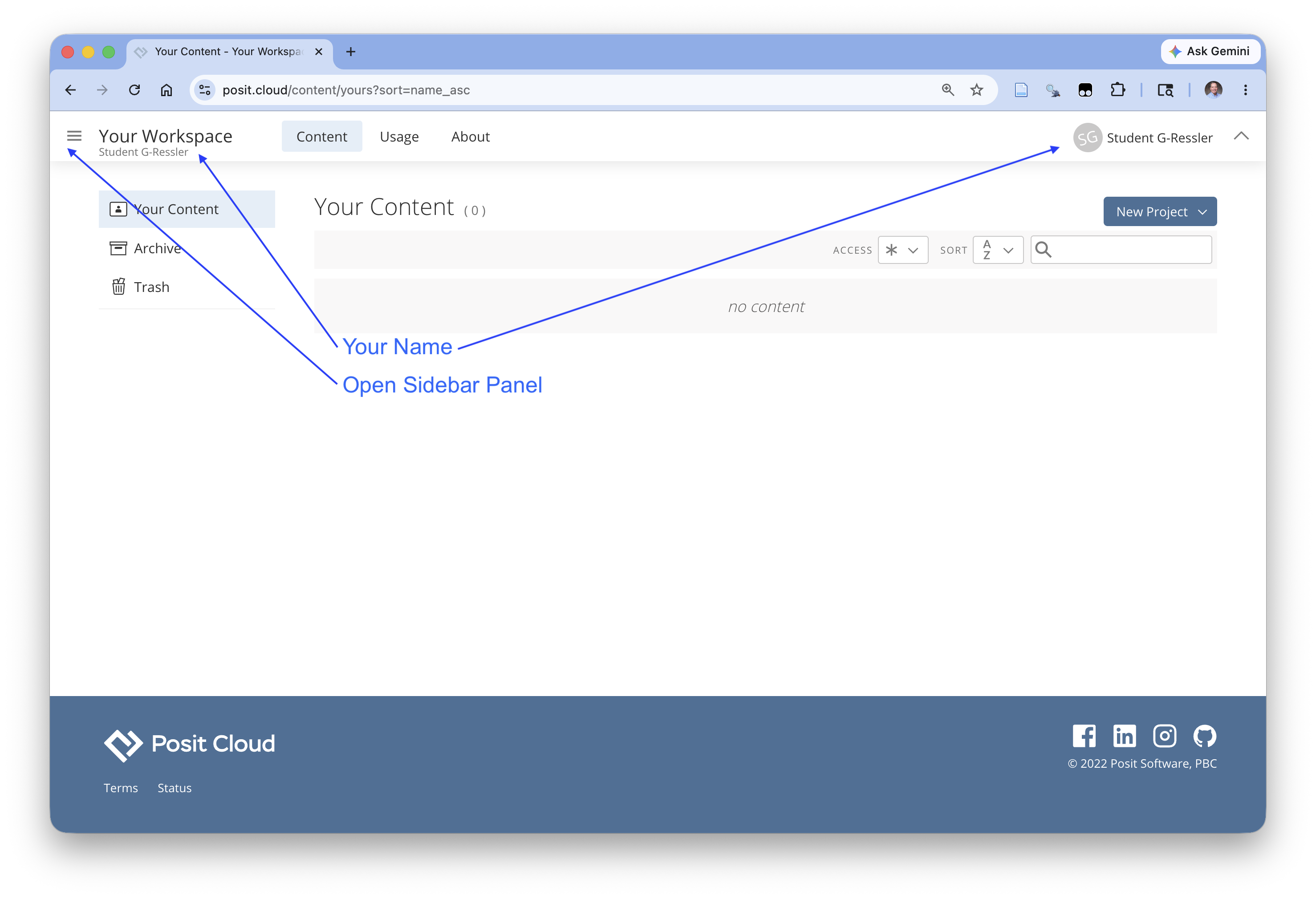
You should see your account name under Your Workspace on the left. This means you are in your personal workspace.
You will not see the course workspace yet as you have to become a member.
1.8.2.2 Join and Access the Course Workspace
This courses uses a Posit Cloud workspace called Intro to DS and AI: 2026.
Click on the link provided by the instructor to join the course workspace.
You should get to a screen that looks like Figure 1.17.
- You may have to log into Posit Cloud.
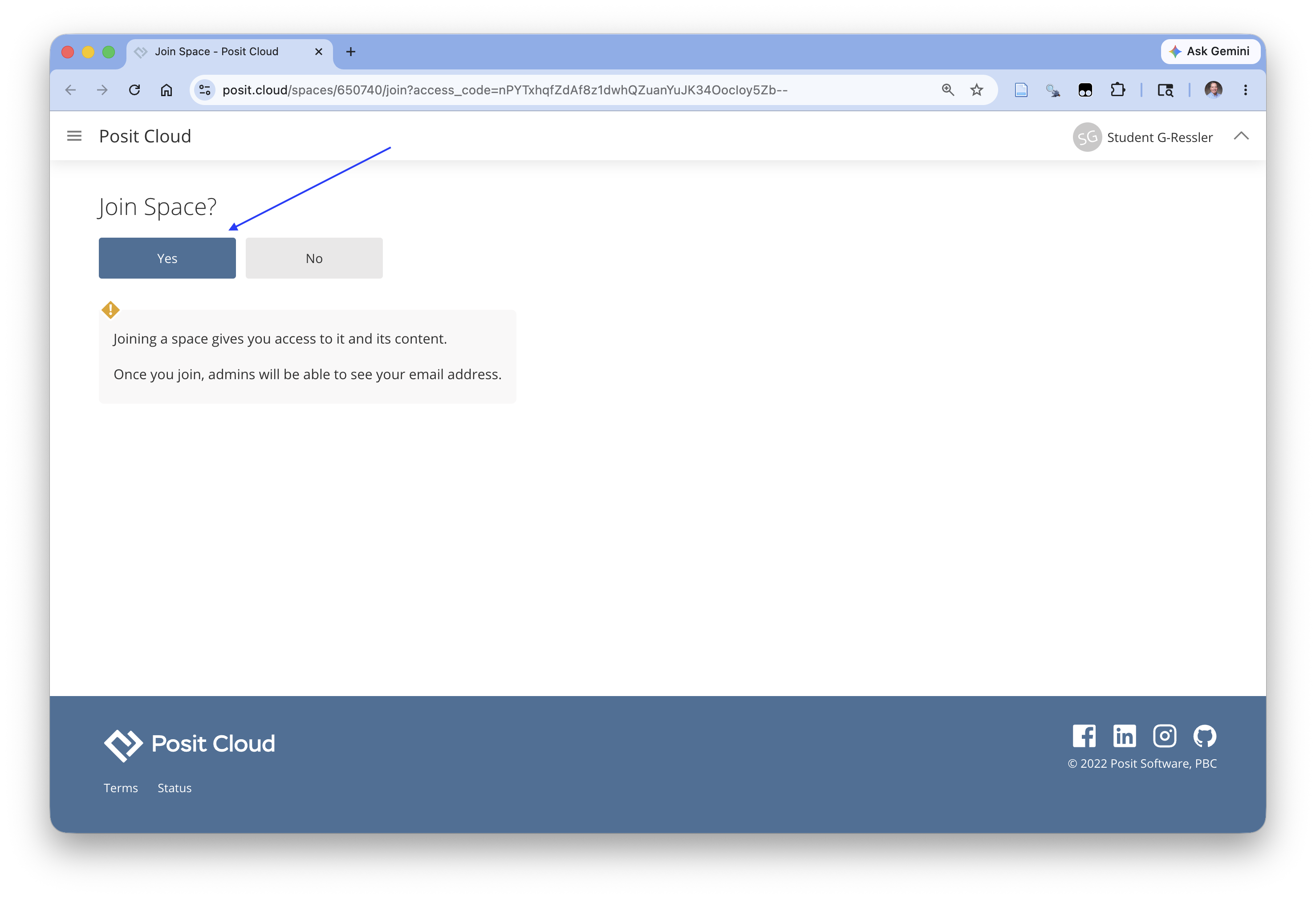
Click Yes and you should get a screen that looks like Figure 1.18
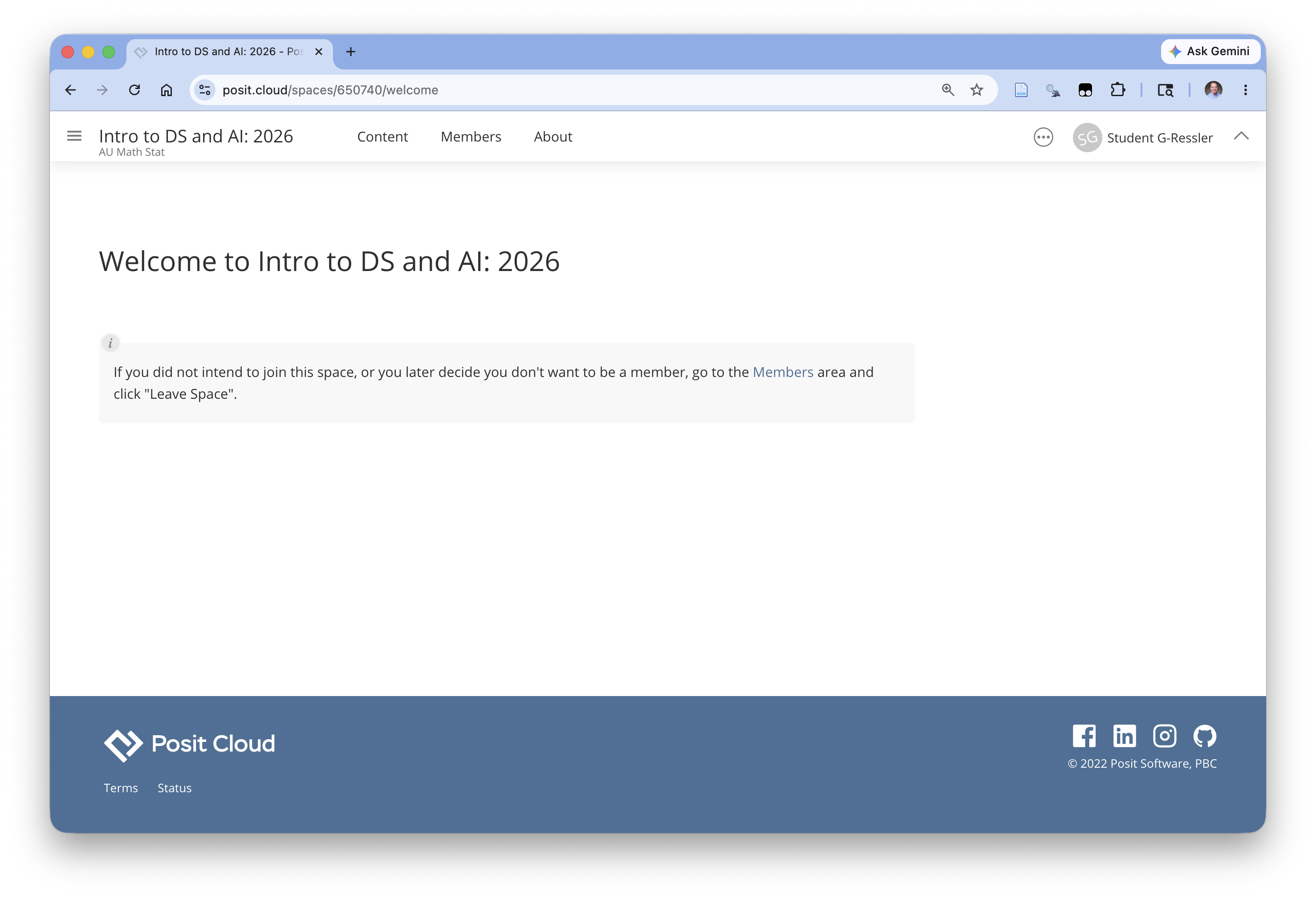
If you click on the icon in the upper left for the sidebar panel (as in Figure 1.16) you can see the course workspace listed under your personal workspace on theft side as in Figure 1.19.

Click on the “Intro to DS and AI: 2026” workspace on the left and/or on Content at the top and you should get a screen like Figure 1.20
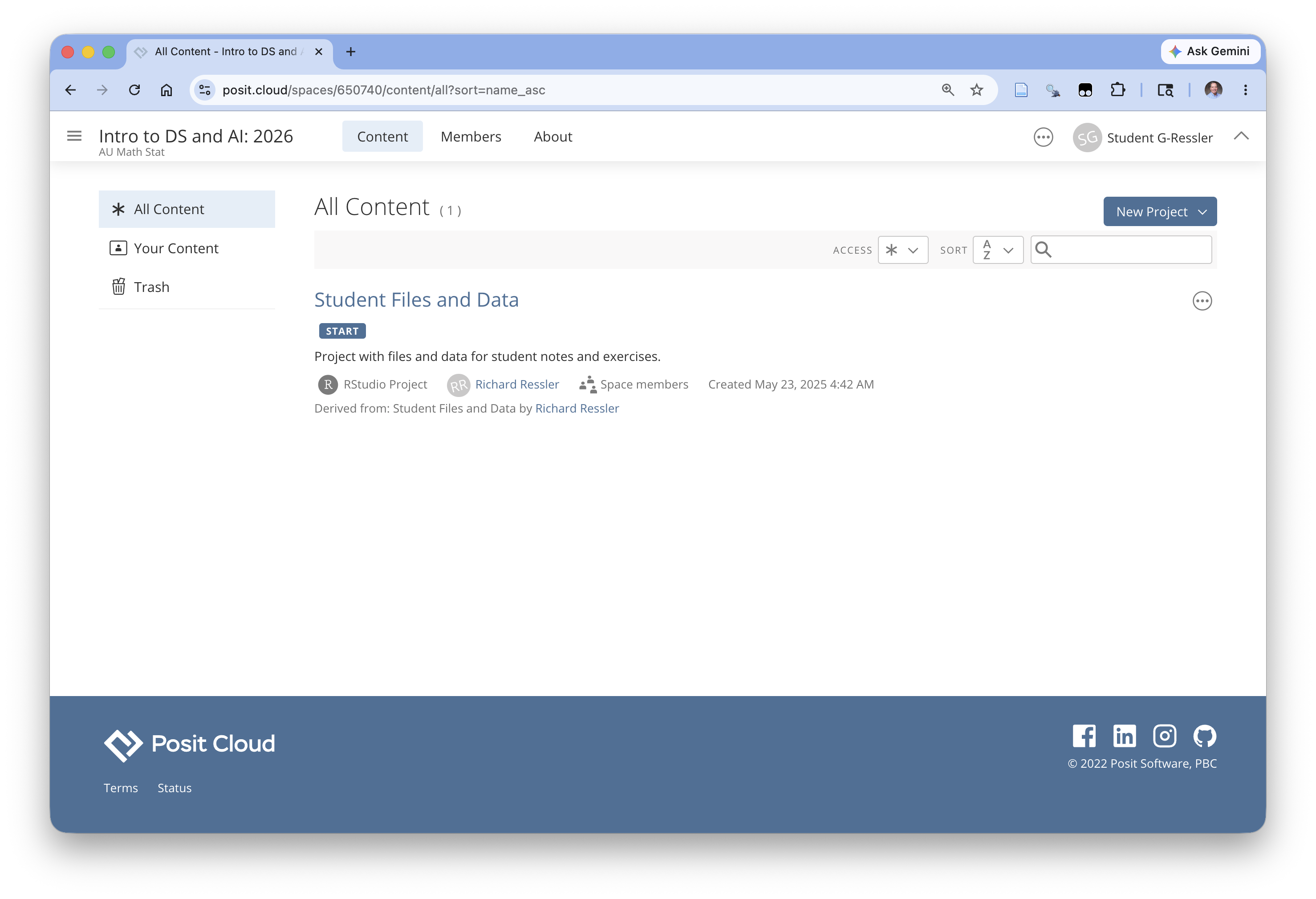
You now have access to the course workspace.
1.8.2.3 Accessing the Student Files and Data Project
This workspace has one project which is called “Student Files and Data”
- This is a project you can use throughout the course to take notes, access some of the data, and write code.
Click on it to deploy the workspace (from a container type infrastructure) and you should get a screen like Figure 1.21
- This may take a few minutes as it is creating an isolated workspace for you with all of the provided files and software.
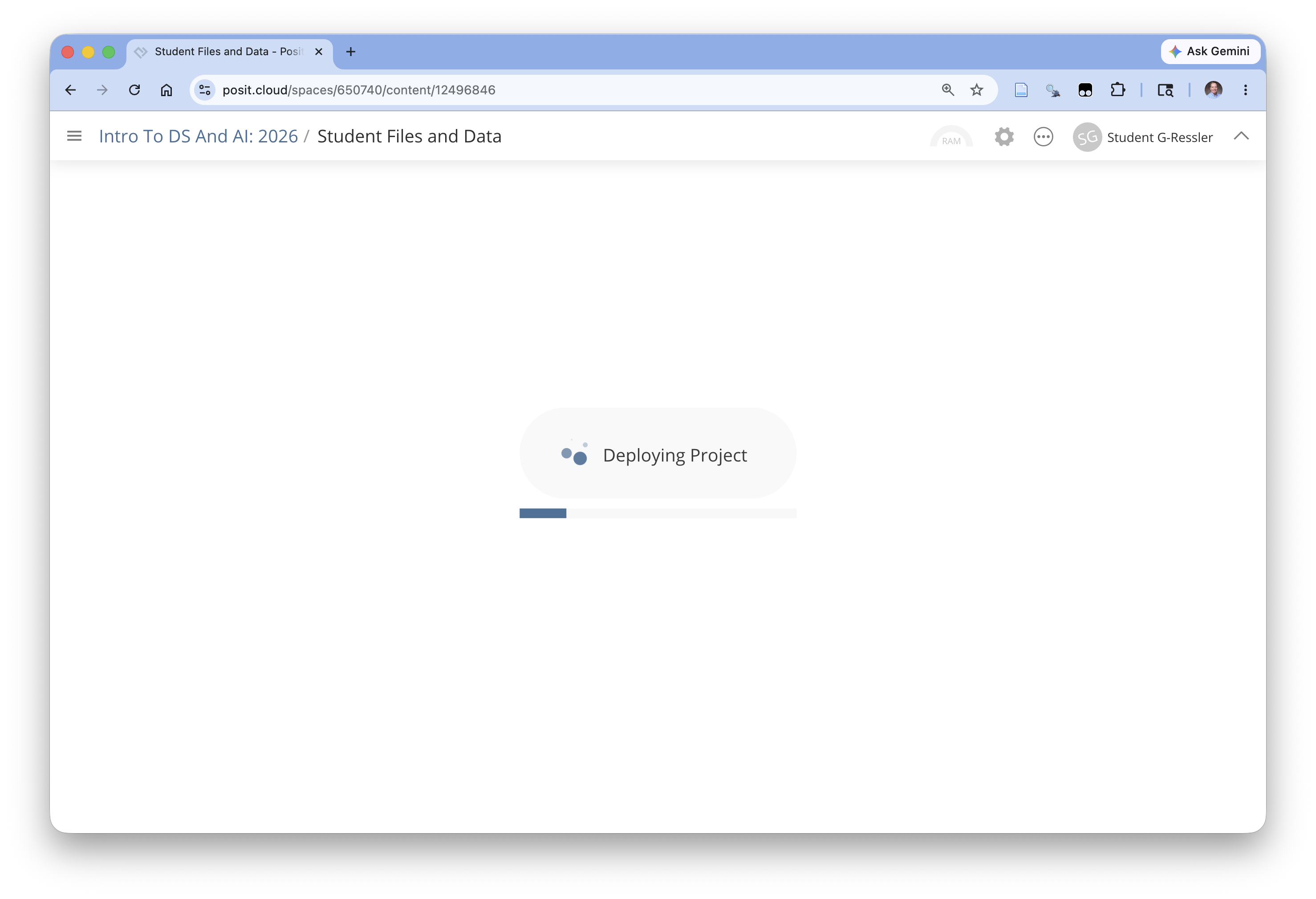
Once the deployment has finished your screen should look like Figure 1.22.
- If the sidebar panel is open, you can close it by clicking on th top of it or the three line menu at the right of the Posit Cloud so you have more screen space for RStudio.
You are now in the RStudio Integrated Development Environment (IDE) as if you had installed the software on your computer.
Important
If you see the words “One or more packages recorded in the lockfile are not installed” in the console, enter renv::restore() after the cursor and hit enter. Say Y when prompted.
- This may take a minute or two to install additional packages.
1.9 Working with RStudio
The RStudio IDE is used by many data scientists as it has lots of features to support literate programming, interactive data science, and software development of which we will use just a few.
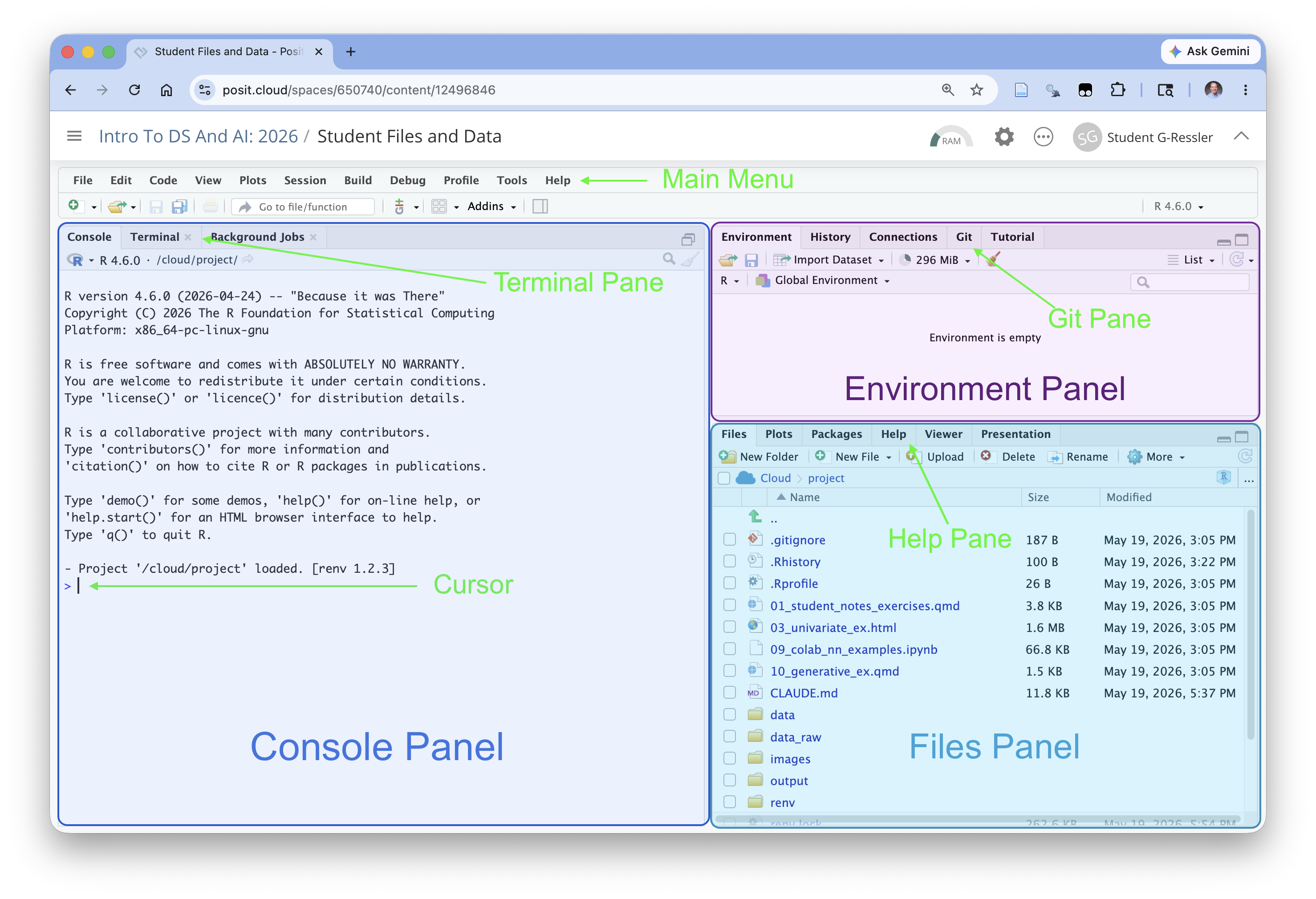
Figure 1.22 shows several important elements of the IDE.
- The main menu at the top is where you can perform almost any action.
- We will not need to use most of these commands as we will be using the shortcut menus.
- However, the tools menu has access to the Keyboard shortcuts list and the Help menu has ready access to Cheat Sheets for the RStudio IDE, R Markdown and several packages.
- The Tools sub-menu includes Global Options where you can customize many aspects of the IDE.
- The Console panel (or pane) provides a command line interface for R.
- One can type R code after the cursor and hit return (enter) to execute the code and see the results.
- Enter 5 + 4 after the cursor to see 9 as the result.
- Later we will use the Terminal tab for interacting with other installed software.
- We will see the Background Jobs tab open and close later as we render a document.
- The Environment panel Environment Tab will show all the objects we create in the Global Environment.
- This includes and data objects or functions that we create.
- The Files Panel Files tab allows us to see all of our files and do basic file management tasks such as rename or delete or copy/move.
- The Help tab will get used a lot.
- Click on the Help tab and enter the word library next to the magnifying glass and hit enter.
- You will see the complete help file for this function.
1.9.1 Open, Edit, and Render a File.
The Files tab shows a number of files, most of which you do need to worry about.
- The .gitignore, .RHistory, and .RProfile are used to track changes in the project.
- The data folder contains several data files we will use later.
- The renv folder, renv.lock file and requirements.txt file are used to manage the R and python packages for the project.
- The student_files_data.RProj file tells RStudio this is an RStudio Project.
The main file of interest is the 01_student_notes_exercises.qmd file.
- This is a Quarto (.qmd) file you can use throughout the course to take notes and do most exercises.
- This is a text-based file that uses Markdown to indicate formatting and other options for the output/
- You can “render” the file into HTML to get a formatted output
Click on the 01_student_notes_exercises.qmd file to open it.
When you open a file, RStudio automatically opens the Source Pane so it looks look similar to Figure 1.23.
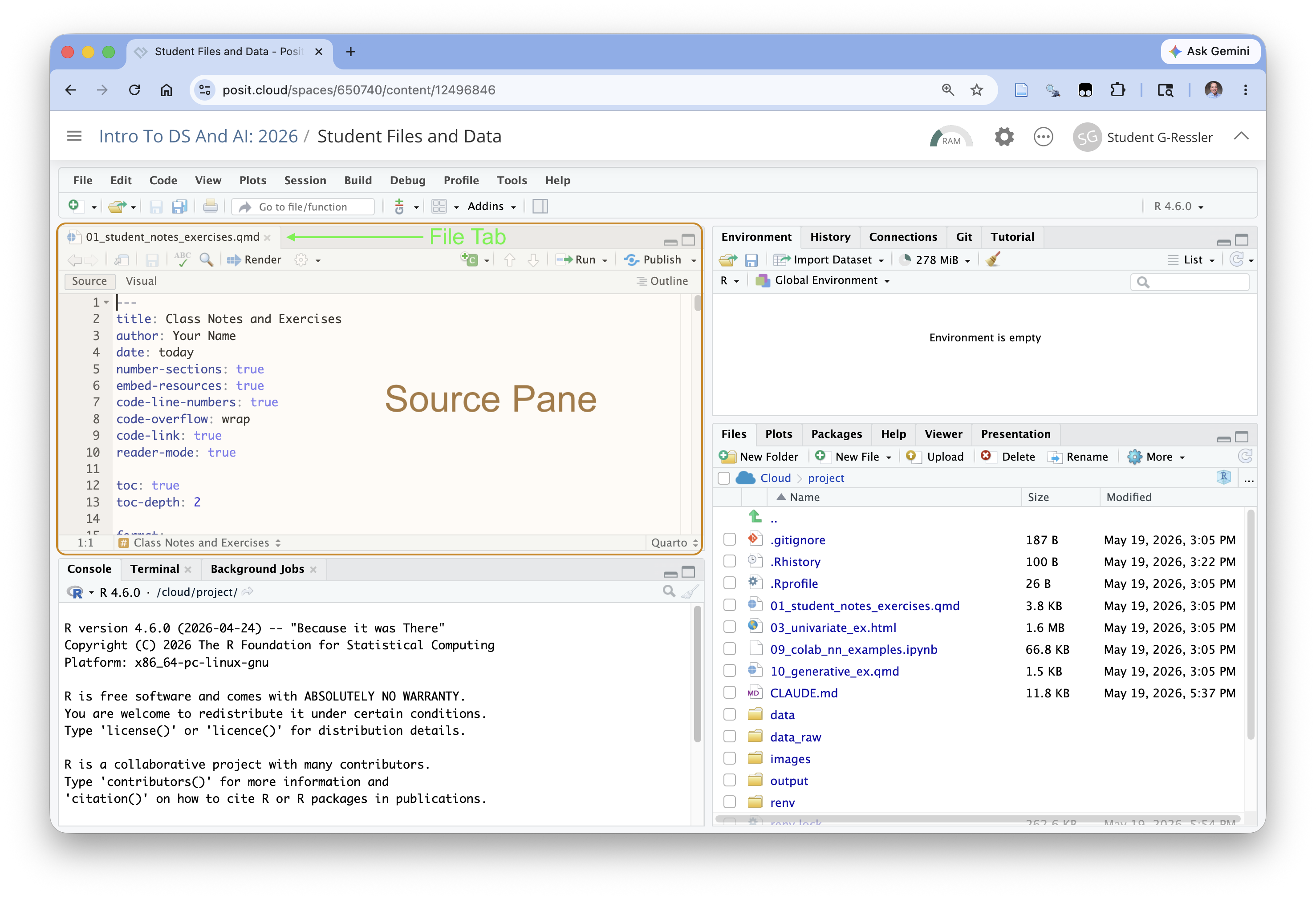
The Source Pane is where you can look at/edit text and code files and view data objects
- You can have multiple tabs open for different files and data objects.
The words Source and Visual (under the shortcuts bar on the left) indicate the active editor.
- The Source editor is a plain-text editor (Figure 1.23), where you write the markdown codes directly.
- This editor is useful for when you are less concerned about formatting or know exactly what you want.
- This editor is the primary editor when writing pure code (
.R) files (R scripts).
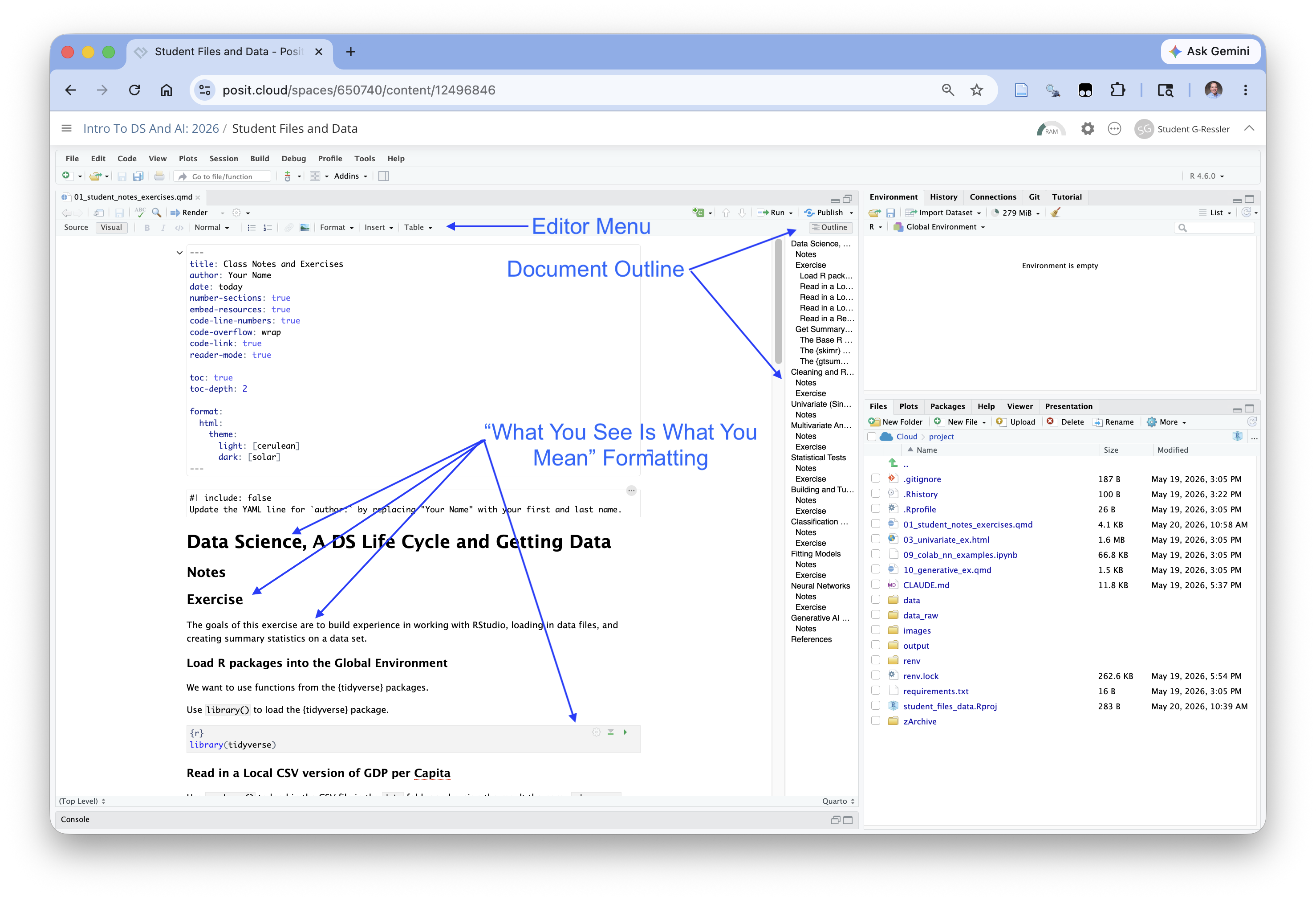
- The Visual editor is a “What You See is What You Mean” editor ( Figure 1.24 ) where you use menus to add formatting elements and want real-time visualization of what your output formatting will generally look like.
- It has multiple menus for inserting R markdown tags into your file, especially use for quarto elements that you might not use very often.
- It also has additional features such as being able to insert citations or special characters.
Figure 1.24 shows a zoomed out view of the visual editor so you can see the editor menu and the formatting style.
- Note this is not exact formatting as it does not include items such as the automated numbering for the headers (which is generated when rendered) and other features such as cross references do not get displayed exactly; it does display the format of the elements based on their markdown tags.
You can use either editor. Most data scientists go back and forth depending upon the tasks.
If you zoom out from the view in Figure 1.23, and collapse the console panel, you can see more of your code in the source editor as in Figure 1.25.
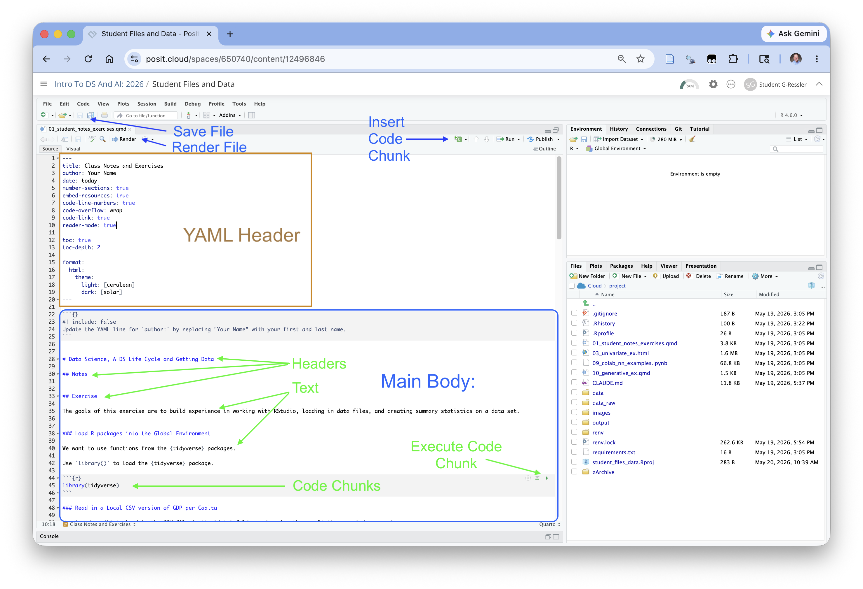
- The shortcuts bar has several important elements.
- The Save icon allows to save your files (which you should do often!).
- The Render arrow will execute the Render function to convert your file into the desired output.
- The Insert Code Chunk button allows you to add new code chunks into the current file at the location of your cursor in the file.
- The Run Code Chunk button gives you options for running one or more code chunks.
- Each code chunk with executable code also has it own Execute Code Chunk arrow.
Since this is a Quarto (.qmd) file it has three kinds of elements
- A single YAML Header at the top
- Main body: one ore more sections of text that may be formatted
- Main Body: one or more executable code chunks
The YAML (Yet Another Markup Language) header is a simple data structure to define and set parameters for working with the files; here they control how the file gets converted to an output format.
- You can see the title of the document and author.
- The next set of YAML “tags” are about formatting the document followed by the table of contents.
- The last set of tags tell Quarto to render the document as an HTML file and then to use the cerulean theme from Bootswatch for HTML documents.
Change the author tag value from “Your Name” to your actual name.
Warning
YAML is very picky about spacing between tags and values and indentation. If you run into errors be sure to check the error message for where there are too few or too many spaces.
Now click on the Render button. It will automatically save your file and try to convert it into a new HTML file, overwriting the last version.
RStudio uses the {quarto} and [knitr} packages to convert the document to a markdown(.md) document and the the {pandoc} package to translate from the markdown forma tot the output format described in the YAML header.
Click on the created HTML file and you should get a pop-up box asking to
OPen in EditororView in Web Browser.View in the Web Browser as we don’t want to edit the raw HTML code.
1.10 R and Markdown Basics
We will be using R and R Markdown to work with our data and keep track of what we are doing in our notebooks.
1.10.1 R Basics
R is a comprehensive programming language for statistical programming.
We will get into more features as we go through the course but it can be helpful to start with some basics.
- R starts counting at 1 (unlike many other languages like Python or C).
[1] 10- R uses standard mathematical operators and order of operations. Use parentheses to help order things.
[1] 14[1] 20[1] 10[1] 512[1] TRUE- R does not care about spaces or line breaks in code, but using appropriate spaces and line breaks can make code more readable.
[1] 14[1] 14[1] 14[1] 14- R is case sensitive as if considers upper case and lower case letters as distinct in variable names and file names.
- R is built out of of objects and allows you to assign names to these objects. R defines several rules for creating legal (“syntactic”) names.
A legal name must:
- Start with a letter (A–Z or a–z)
- That is followed by letters, numbers, . (dot), or _ (underscore), with no spaces
- Not be a reserved keyword (like if, for, TRUE, etc.)
Recommend using “snake_case” for longer names instead of . in the name (that is older style)
If a name is non-syntactic, e.g., has spaces in it (which happens a lot on real-world data), R allows you to use a ` (a tic or grave accent (U+0060), not a single quote) on both ends of the name to make it legal.
[1] 1 2 3[1] 10 20 30- R has a built-in symbol for missing values:
NA.
- Any operation that includes an
NAvalue will returnNA. - Many built in functions allow you to remove the
NAs before the calculations are made so can get a non-NAresult.
- R has a built-in operator called the native pipe for “chaining” operations.
- Very useful in connecting lines of code (or a series of operations) together instead of trying to fit on one line.
- Putting functions calls on new lines is typical in tidyverse style as you can see the Flow of the data through the code.
- This a trivial example. We will see more typical uses in Section 2.3.2.
- Many R functions are “vectorized” meaning they work on each element of a vector in turn without having to write extra code.
[1] 2 4 6[1] TRUE FALSE FALSE[1] 1 4 9
Warning
R uses a construct called “recycling” to match up elements one-to-one in the two vectors to do these operations.
- It works as expected when one vector has multiple elements and the other vector either has one element or the same number of elements as the other vector. The one element gets “recycled” for each element in the longer vector.
- It can get confusing, (R will issue a “warning”) when the vectors have different numbers of elements as the shorter vector elements get recycled and “start over” unexpectedly.
[1] 2 6 6[1] FALSE FALSE FALSEWhen trying to see if the elements in one vector are present in another of different length, say check if a vector of two municipalities is in another vector of five municipalities, it is much better to use the %in% function instead of ==.
- The
#is the “comment” character in R. Once R hits a#on a line it stops reading the rest of the line.
- Commenting out lines is a good way to add notations to the code explaining what you are doing next.
- It is also useful in debugging if you want to stop certain line of code from running.
- The
$operator in R is shorthand for the[[]]extraction operator for named variables. It is commonly used with data frames to get a single column as a vector.
Rows: 32
Columns: 11
$ mpg  <dbl> 21.0, 21.0, 22.8, 21.4, 18.7, 18.1, 14.3, 24.4, 22.8, 19.2, 17.8,…
$ cyl  <dbl> 6, 6, 4, 6, 8, 6, 8, 4, 4, 6, 6, 8, 8, 8, 8, 8, 8, 4, 4, 4, 4, 8,…
$ disp <dbl> 160.0, 160.0, 108.0, 258.0, 360.0, 225.0, 360.0, 146.7, 140.8, 16…
$ hp   <dbl> 110, 110, 93, 110, 175, 105, 245, 62, 95, 123, 123, 180, 180, 180…
$ drat <dbl> 3.90, 3.90, 3.85, 3.08, 3.15, 2.76, 3.21, 3.69, 3.92, 3.92, 3.92,…
$ wt   <dbl> 2.620, 2.875, 2.320, 3.215, 3.440, 3.460, 3.570, 3.190, 3.150, 3.…
$ qsec <dbl> 16.46, 17.02, 18.61, 19.44, 17.02, 20.22, 15.84, 20.00, 22.90, 18…
$ vs   <dbl> 0, 0, 1, 1, 0, 1, 0, 1, 1, 1, 1, 0, 0, 0, 0, 0, 0, 1, 1, 1, 1, 0,…
$ am   <dbl> 1, 1, 1, 0, 0, 0, 0, 0, 0, 0, 0, 0, 0, 0, 0, 0, 0, 1, 1, 1, 0, 0,…
$ gear <dbl> 4, 4, 4, 3, 3, 3, 3, 4, 4, 4, 4, 3, 3, 3, 3, 3, 3, 4, 4, 4, 3, 3,…
$ carb <dbl> 4, 4, 1, 1, 2, 1, 4, 2, 2, 4, 4, 3, 3, 3, 4, 4, 4, 1, 2, 1, 1, 2,…
 [1] 21.0 21.0 22.8 21.4 18.7 18.1 14.3 24.4 22.8 19.2 17.8 16.4 17.3 15.2 10.4
[16] 10.4 14.7 32.4 30.4 33.9 21.5 15.5 15.2 13.3 19.2 27.3 26.0 30.4 15.8 19.7
[31] 15.0 21.4
 [1] 21.0 21.0 22.8 21.4 18.7 18.1 14.3 24.4 22.8 19.2 17.8 16.4 17.3 15.2 10.4
[16] 10.4 14.7 32.4 30.4 33.9 21.5 15.5 15.2 13.3 19.2 27.3 26.0 30.4 15.8 19.7
[31] 15.0 21.4
1.10.2 R Markdown Basics
“Markdown is a plain text format that is designed to be easy to write, and, even more importantly, easy to read.”
Markdown is used in the Text portions of the document to describe how to format the text.
- Use
#to denote headers#is header 1,##header 2, and###header 3 and so on. - Be sure to leave a blank line before any header.
- You can create bullets using
-and use indents to create sub bullets. - Be sure to leave a blank line between a non-bullet line and the first line of bullets.
- To create a code chunk, use “```” in the line before the code and in the line after the code.
- Put the name of the coding language in the chunk after the upper “```”
Quarto supports both HTML and PDF, so there is great flexibility in output.
- However, HTML can support interactivity, e.g., click on multiple tabs, but PDF does not.
- Be careful in how much you customize your document for one or the other unless you know you will only be using a single format.
You can use the visual editor to implement many R markdown tags and then check them in the Source editor.
For an longer introduction to R Markdown, see Markdown Basics
1.11 Exercise 01: Working with RStudio and R: Getting and Summarizing Data
The goals of this exercise are to build experience in working with RStudio, loading in data files, and creating summary statistics on a data set.
- If it is not already open, click on the
01_student_notes_exercises.qmdfile in the files tab in the Files pane.
The file should be visible in the Source panel of RStudio with the tool bar at the top like in Figure 1.26.

1.11.1 Load R packages into the Global Environment
The Global Environment has the list of names of every object we can work with be it a function or data.
When RStudio starts, it automatically loads Base R and its common packages into the Global Environment.
- You can see them by clicking on the down arrow to the right of
Global Environmentin theEnvironmentTab. - These packages provide essential functions for many projects in R.
- Once other packages have been installed on your computer, you use the
library()function to load additional packages into your global environment so you have easy access to the functions in each package.
We want to use functions from the {tidyverse} packages.
- We can use
library()to load the {tidyverse} package since has already been installed. - The {tidyverse} package includes many other packages for working with data.
- The {readr} package has functions to read in a variety of file types including
read_csv().
- You can see the response shows several of the packages of interest and their versions.
- The conflicts are where functions in the {tidyverse} packages have the same names as functions in Base R so to avoid confusion, the Base R functions will be dropped from the search string.
1.11.2 Read in a Local CSV version of GDP per Capita 2023 Data
Look at the Files tab to see the current file structure.
- If you click on the
datafolder you should see several versions of the GDP per Capita data we looked at earlier.
- Let’s use
read_csv()to load in the CSV file. We will use the R assignment arrow<-to assign the namegdp_pc_csvto the data.
- Click on the green arrow all the way to the right of the code chunk below to run the code chunk
- A keyboard shortcut is to put your cursor in a line of code an hit
CMD+Return(Mac) orCTRL+Enter(Windows)
- We got a response that it successfully read in 61 rows from four columns.
Since each “column” is also a named “variable”, I will use the terms “column” and “variable” interchangeably for now.
Let’s break apart the code we just saw from right to left.
"./data/gdp_per_capita_2023.csv"is the path and name of the file we want to read in.- The path is
./datawhich means start from the current directory (where this file is located) and go down into thedatadirectory. - The
gdp_per_capita_2023.csvis the name of the file we want.
- The path is
read_csv()is name of function we are using to load in the data.- The
file =is the first argument in the function which requires “Either a path to a file, a connection, or literal data (either a single string or a raw vector)”. - One of the nice features about R and Tidyverse is their strong help system.
- Use the
Helptab to search forread_csv(no parens) or enter ?read_csv into the console prompt and the help file for the function should appear in theHelptab. - You can see all the arguments for a function with explanations for each argument and usually code examples at the bottom.
- The
<-is the assignment arrow which means take the result from the right of me and give it the name on the left of me.gdp_pc_csvis the name we assigned to the data we read in.- We can see it in the
Environmenttab which lists all the objects in the global environment. - It is under the
Datacategory.
- We can see it in the
Let’s look at the data object we created.
- Go to the
Environmenttab and click on the blue downward facing arrow to the left of the name.- You will see the name of each of the variables (the columns) and their class and length.
- Since this is rectangular data, all the variables are the same length, 61.
- The first variable is of class
chrwhich means character data. Character data is always in quotes""or''. - The other three variables are of class
numwhich is short fornumeric- a catch-all class for bothintegeranddouble.
- Now click on the name
gdp_pc_csvin theEnvironmenttab and a new tab will open in the Source panel where you can see all of the data.- You can also use the
View(object_name)function in the console where you replace object_name with the actual name.
- You can also use the
- You can sort by individual columns or filter by column values.
- Filter on
gov_entityto just those that have adin the name and sort by population.- This is not changing the actual data, just what you are looking at.
- Put the name of the variable into the following code chunk and run the chunk by using the green arrow or clicking on the name and using the
CMD+Return(Mac) orCTRL+Enter(Windows) shortcut.
# A tibble: 61 × 4
   gov_entity population general_revenue_per_person average_revenue_per_person
   <chr>           <dbl>                      <dbl>                      <dbl>
 1 Dimal           28135                      14856                      28307
 2 Pogradec        46070                      15146                      28307
 3 Prrenjas        18768                      15466                      28307
 4 Kurbin          34405                      16134                      28307
 5 Berat           62232                      16889                      28307
 6 Krujë           51191                      17127                      28307
 7 Kuçovë          31077                      17132                      28307
 8 Belsh           17123                      17183                      28307
 9 Cërrik          25163                      17277                      28307
10 Devoll          25897                      18446                      28307
# ℹ 51 more rows- RStudio will display all the data along with the class of the data object.
- You can see it is a “tibble” with 61 rows and four columns. We will talk more about tibbles in a few minutes.
- You can use the buttons at the bottom to page through the data and see all the values.
Now use the green square in the tool bar (Figure 1.26) to insert an R code chunk and use the function glimpse(object_name) to see another view of the data.
- You can also use a keyboard shortcut. See Help Keyboard Shortcuts Help (Be sure the language option is
r)
Rows: 61
Columns: 4
$ gov_entity                 <chr> "Dimal", "Pogradec", "Prrenjas", "Kurbin", …
$ population                 <dbl> 28135, 46070, 18768, 34405, 62232, 51191, 3…
$ general_revenue_per_person <dbl> 14856, 15146, 15466, 16134, 16889, 17127, 1…
$ average_revenue_per_person <dbl> 28307, 28307, 28307, 28307, 28307, 28307, 2…- This shows you all the columns, the names of each column, their class and as many values as will fit on the page.
glimpse()is handy when you have a lot of columns and you want to see them all on the page instead of scrolling across a page
1.11.3 Read in a Local XLSX version of GDP per Capita 2023 Data
To read in Excel files, we need to load a new package called {readxl}
Insert a code chunk and use library() to load the {readxl} package.
Now insert a code chunk and use the read_xlsx() function to read in the file from data and assign the name gdp_pc_xlsx to it.
This function does not return a result but you can see the new data object in the Environment tab.
- It has 61 observations (rows) and 4 variables (columns) as expected.
If you look at help you notice there is a sheet argument so you can identify which sheet you want to read in. It defaults to the first sheet if not used.
1.11.4 Read in a Local JSON version of GDP per Capita 2023 Data
To read in JSON files, we need to load a new package called {jsonlite}
Insert a code chunk and use library() to load the {jsonlite} package.
- You got a response warning of a conflict with another function. We do not need to worry about that.
Now insert a code chunk and use the read_json() function to read in the file from data and assign the name gdp_pc_json to it.
- This will read in and convert relatively simple JSON files to data frames.
This function does not return a result but you can see it the new data object in the Environment tab.
- Notice this object is called a “List”, which is a non-rectangular data structure.
- You can see all the data is there but now how we want it.
Looking at help, let’s use the simplifyVector argument and set it to TRUE (ALL CAPS).
- Now we see the expected 61 observations and 4 variables.
1.11.5 Read in a Remote CSV version of GDP per Capita 2023 Data
There is a CSV version of the data on a public web site on the cloud repository GitHub at https://github.com/AU-datascience/data/tree/main/intro_ds_ai_mini.
We can use read_csv(file="URL") to read CSV files from websites that allow it. We replace the “URL” with the actual URL address for the CSV file.
- Here the URL is https://raw.githubusercontent.com/AU-datascience/data/refs/heads/main/ds_ai_mini/gdp_per_capita_2023.csv.
To make our code a bit easier to read, we are going to create a new object where we assign a name to the URL and use the named object in the read_csv() function.
- Note that the
my_urlnow appears as under theValuesin the environment. - It meets the requirements for the
fileargument as it is a complete path to a file that just happens to be remote. - The resulting
gdp_pc_csv_urlobject has the same 61 observations and 4 variables as all the others as we would expect.
1.11.6 Saving and Compressing Your Data
You can also save your data by “writing” out in a variety of formats to facilitate sharing across project or with other people who may not be R users.
The syntax is similar for the functions from different packages shown in the code below.
- You can adjust the path
./outputs/to wherever you want, but it is good practice to separate the output from your code files.
R also has its own compressed binary file format (.rds) (that is especially good for shrinking the size of your data file and it is much faster to read in. However it only stores one object and is not useful outside of R.
- You will note this file is actually larger than the CSV format but that is because this is such a small data set. You will see the .rds can be much smaller for larger data sets.
R has the RData format which allows you to store all the objects in your environment in one binary file. By using save(), and load(), you can share your environment for later use.
Finally, you can also use R’s zip() function to compress a file or folder of files you have already created for sharing.
1.11.7 Getting Summary Statistics about the Data
We have already seen some “metadata” (data-about-data) for the data. We know how many observations and columns there are in the data set and the classes of the variables.
1.11.8 The Base R summary() Function
Now let’s get information about values of the data using the Base R summary() function.
     gov_entity   population     general_revenue_per_person
 Length   :61   Min.   :  1843   Min.   : 14856
 N.unique :61   1st Qu.: 10750   1st Qu.: 20845
 N.blank  : 0   Median : 19261   Median : 26377
 Min.nchar: 3   Mean   : 39382   Mean   : 30545
 Max.nchar:14   3rd Qu.: 34405   3rd Qu.: 36423
                Max.   :598176   Max.   :100942
 average_revenue_per_person
 Min.   :28307
 1st Qu.:28307
 Median :28307
 Mean   :28307
 3rd Qu.:28307
Max. :28307 - The first variable is of class “character” so is non-numeric which means no numerical statistics.
- The remaining three variables are numeric so we can see 6 statistics about the values.
- Min: the minimum value
- 1st Qu: the 1st quartile - the value at which 25% of the observations have lower values.
- Median: the 2nd quartile - the value at which 50% of the data has lower values and 50% has higher values. One measure of the “middle” of the data.
- Mean: the arithmetic mean (average) of the values. Another measure of the “middle” of the data.
- 3rd Qu: The the 3rd quartile - the value at which 75% of the observations have lower values.
- Max: the maximum value.
These statistics allow us to have some insights about the center of the distribution of the data and the range and spread of the data.
The GDP data is complete in the sense there are no missing values - denoted in R as NA for “not available”.
Let’s use summary on the Base R data set penguins which is not complete.
      species          island       bill_len        bill_dep
 Adelie   :152   Biscoe   :168   Min.   :32.10   Min.   :13.10
 Chinstrap: 68   Dream    :124   1st Qu.:39.23   1st Qu.:15.60
 Gentoo   :124   Torgersen: 52   Median :44.45   Median :17.30
                                 Mean   :43.92   Mean   :17.15
                                 3rd Qu.:48.50   3rd Qu.:18.70
                                 Max.   :59.60   Max.   :21.50
                                 NAs    :2       NAs    :2
  flipper_len      body_mass        sex           year
 Min.   :172.0   Min.   :2700   female:165   Min.   :2007
 1st Qu.:190.0   1st Qu.:3550   male  :168   1st Qu.:2007
 Median :197.0   Median :4050   NAs   : 11   Median :2008
 Mean   :200.9   Mean   :4202                Mean   :2008
 3rd Qu.:213.0   3rd Qu.:4750                3rd Qu.:2009
 Max.   :231.0   Max.   :6300                Max.   :2009
NAs :2 NAs :2 - Now we see the columns
species,island, andsexhave a discrete number of values and their counts but no statistics.- These are categorical variables which are of class “factor” in R. These only have a limited number of values or levels.
- Factors actually are coded as integers but we just deal with the level names and R treats them differently than numbers, if if the level names look like a number, e.g.,
1stands for Male and2stands for Female.
- We also see that the numerical variables now have a row for the number of missing values (
NA's) for each variable.
The Base R summary() function gives us the basics. Other packages have created their own summary style functions to provide more information.
1.11.9 The {skimr} Package
The {skimr} package’s skim() function provides more statistics than Base R’s summary().(Waring et al. 2025)
- These include the
complete_rate(% not-missing), the standard deviation, and a simple “character” plot on the right showing the distribution of the values. - The {skimr} package also has more options for formatting the output than
summary().
Let’s skim the GDP data.
| Name | gdp_pc_csv |
| Number of rows | 61 |
| Number of columns | 4 |
| _______________________ | |
| Column type frequency: | |
| character | 1 |
| numeric | 3 |
| ________________________ | |
| Group variables | None |
Variable type: character
| skim_variable | n_missing | complete_rate | min | max | empty | n_unique | whitespace |
|---|---|---|---|---|---|---|---|
| gov_entity | 0 | 1 | 3 | 14 | 0 | 61 | 0 |
Variable type: numeric
| skim_variable | n_missing | complete_rate | mean | sd | p0 | p25 | p50 | p75 | p100 | hist |
|---|---|---|---|---|---|---|---|---|---|---|
| population | 0 | 1 | 39381.74 | 79060.56 | 1843 | 10750 | 19261 | 34405 | 598176 | ▇▁▁▁▁ |
| general_revenue_per_person | 0 | 1 | 30544.52 | 16002.56 | 14856 | 20845 | 26377 | 36423 | 100942 | ▇▃▁▁▁ |
| average_revenue_per_person | 0 | 1 | 28307.00 | 0.00 | 28307 | 28307 | 28307 | 28307 | 28307 | ▁▁▇▁▁ |
- Note the extra results and the fact that it is now in tibbles, not just printed on the screen.
- Also note we did not use
library()to load the package.- Since we only needed access to one function in the package, we are using the
::operator which is interpreted as for “Use the function on the right of the::from the package on the left of the::”.
- Since we only needed access to one function in the package, we are using the
Let’s skim() penguins.
| Name | penguins |
| Number of rows | 344 |
| Number of columns | 8 |
| _______________________ | |
| Column type frequency: | |
| factor | 3 |
| numeric | 5 |
| ________________________ | |
| Group variables | None |
Variable type: factor
| skim_variable | n_missing | complete_rate | ordered | n_unique | top_counts |
|---|---|---|---|---|---|
| species | 0 | 1.00 | FALSE | 3 | Ade: 152, Gen: 124, Chi: 68 |
| island | 0 | 1.00 | FALSE | 3 | Bis: 168, Dre: 124, Tor: 52 |
| sex | 11 | 0.97 | FALSE | 2 | mal: 168, fem: 165 |
Variable type: numeric
| skim_variable | n_missing | complete_rate | mean | sd | p0 | p25 | p50 | p75 | p100 | hist |
|---|---|---|---|---|---|---|---|---|---|---|
| bill_len | 2 | 0.99 | 43.92 | 5.46 | 32.1 | 39.23 | 44.45 | 48.5 | 59.6 | ▃▇▇▆▁ |
| bill_dep | 2 | 0.99 | 17.15 | 1.97 | 13.1 | 15.60 | 17.30 | 18.7 | 21.5 | ▅▅▇▇▂ |
| flipper_len | 2 | 0.99 | 200.92 | 14.06 | 172.0 | 190.00 | 197.00 | 213.0 | 231.0 | ▂▇▃▅▂ |
| body_mass | 2 | 0.99 | 4201.75 | 801.95 | 2700.0 | 3550.00 | 4050.00 | 4750.0 | 6300.0 | ▃▇▆▃▂ |
| year | 0 | 1.00 | 2008.03 | 0.82 | 2007.0 | 2007.00 | 2008.00 | 2009.0 | 2009.0 | ▇▁▇▁▇ |
1.11.10 The {gtsummary} Package
The {gtsummary} package provides “an elegant and flexible way to create publication-ready analytical and summary tables using the R programming language.” (Sjoberg et al. 2021)
Use gtsummary::tbl_summary(gdp_pc_csv[,2:4]) to create a summary table of the GDP data.
| Characteristic | N = 611 |
|---|---|
| population | 19,261 (10,750, 34,405) |
| general_revenue_per_person | 26,377 (20,845, 36,423) |
| average_revenue_per_person | |
| 28307 | 61 (100%) |
| 1 Median (Q1, Q3); n (%) | |
Important
Here the code uses some new syntax at the end of the variable name [,2:4] so the calculations do not include the first column which is no numeric: gov_enty.
- This is showing another feature of R - the ability to use only a subset of the entire data set with some compact syntax.
- Interpret the syntax of the
[]operators as saying, subset the data on the left to use all the rows (the,) and only columns 2 through 4, the2:4 - This means all 61 rows but only columns 2, 3 and 4 are used by the function.
- We did this to avoid have a very long table with just the names of each
gov_entyfor the first 61 rows.
Now let’s do a summary of the penguins data set.
| Characteristic | N = 3441 |
|---|---|
| species | |
| Adelie | 152 (44%) |
| Chinstrap | 68 (20%) |
| Gentoo | 124 (36%) |
| island | |
| Biscoe | 168 (49%) |
| Dream | 124 (36%) |
| Torgersen | 52 (15%) |
| bill_len | 44.5 (39.2, 48.5) |
| Unknown | 2 |
| bill_dep | 17.30 (15.60, 18.70) |
| Unknown | 2 |
| flipper_len | 197 (190, 213) |
| Unknown | 2 |
| body_mass | 4,050 (3,550, 4,750) |
| Unknown | 2 |
| sex | |
| female | 165 (50%) |
| male | 168 (50%) |
| Unknown | 11 |
| year | |
| 2007 | 110 (32%) |
| 2008 | 114 (33%) |
| 2009 | 120 (35%) |
| 1 n (%); Median (Q1, Q3) | |