9 Neural Networks

Published

May 23, 2025

Keywords

Neural Networks, Layers, Weights, Biases, Back Propagation, reticulate, TensorFlow, Keras, CNNs

9.1 Introduction

This module introduces neural networks and the basics of their structure and algorithms.

Learning Outcomes

Explain the basic architecture of a neural network.
Explain the role of back-propagation and gradient descent.
Build a basic neural network using R.
Describe a Convolutional Neural Network.

9.1.1 References

9.2 Neural Networks

Deep Learning and Neural Nets are two terms that describe a set of machine learning methods that build networks with one or more layers of calculations to manipulate input data to derive outputs.

The Deep in Deep Learning refers to the use of multiple layers in the networks. The more layers of calculations, the deeper the network.
The Neural in Neural Networks (Neural Nets) refers to the use of methods called Artificial Neural Networks whose design is inspired by or emulates the actions of nerves in animals.
- Nerves receive inputs from multiple chemical signals and when the level of signal crosses a threshold, the nerve can “fire”.
- When a nerve reaches its action potential and fires, it sends electro-chemical signals cascading down the nerve to generate outputs.
- These outputs generate input signals to other (nearby) nerves (or other cells).
- These signals can either trigger the activation in nearby nerves or suppress their activation.
- The outputs may also cause a cell to take or suppress a given activity.
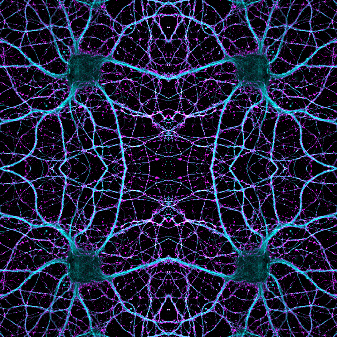
Figure 9.1 shows an image of several nerve cells and their growing network of connections across the brain.

Figure 9.1: Nerve Cells that are connecting to each other with multiple neurons. (Institute (2017))

For more insights into animal neurons and their firing, see the following video (Neuroscientifically Challenged 2014)

Deep Learning methods can used for supervised or unsupervised learning.

They tend to require lots of input data and many calculations so their development has expanded greatly in the last few years given the large increases in available data and affordable computing power.

Note

Deep Learning and Neural Nets have evolved in both computing and statistical domains and combine aspects of networks and statistical methods and transformations. Thus they tend to use different terms describing the same concepts, e.g., “features” are “predictors” are “inputs.”

9.2.1 A Single-Layer Neural Network

Neural networks are still trying to estimate the true but unknown function that defines the relationship between one set of data and another.

In the case of supervised learning, the relationship is between at set of input “features” (variables) \(X = X_1, \ldots, X_n\), the inputs, and a \(Y\) the response or output.

The goal is to approximate the true but unknown function that maps \(X \mapsto Y\) as accurately as possible.

One way to do this is through a neural network, which builds this relationship by passing inputs through one or more layers of intermediate computations, ultimately producing a predicted output.

Similar to boosted trees, the layers may have multiple nodes where each node is “weak”, but the combination of multiple nodes in the layer can generate “strong” (useful) results.

Figure 9.3 depicts a single layer neural network with

input nodes on the left, one for each predictor \(X_1, X_2, X_3, and X_4\)
a single “hidden” layer with multiple “units” (nodes), and
an output layer on the right which generates the final prediction \(\hat{Y}\).

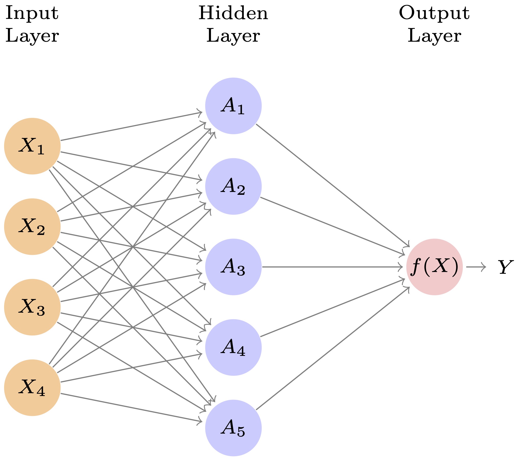
Figure 9.3: A single layer neural network

The arrows from the inputs to the units (nodes) in the middle layer indicate each input is fed to a middle layer unit that will then combine all the inputs it receives.
- The number of units in a hidden layer, \(K\), is a tuning parameter (to be discussed later).
Each unit applies a specific transformation to the inputs and sends its output to the final layer, which combines those \(K\) outputs into a prediction.

Note

The terms units, nodes, or “perceptrons” all refer to the individual elements of a network layer.

9.2.1.1 Weights and Biases - the Neural Network Analogs to Regression Coefficients

What distinguishes a neural network from other methods is the way the hidden layers make calculations on the inputs and the final layer then combines the outputs from the previous layer, (inputs to the final layer), to calculate a final prediction.

To understand what happens inside a neural network, it helps to think in terms familiar from linear regression.

In a basic linear regression, we model:

\[Y = \beta_0 + \beta_1 X_1 + \beta_2 X_2 + \dots + \beta_p X_p + \varepsilon \tag{9.1}\]

or, using the \(\sum\) symbol

\[Y = \beta_0 + \sum_i\beta_iX_i \tag{9.2}\]

To put Equation 9.1 and Equation 9.2 in the context of neural networks,

The coefficients \(\beta_j\) are “weights” that indicate how important each feature is to predicting \(Y\).
The intercept \(\beta_0\) acts like a constant shift — a baseline level when all \(X_j = 0\)..

Neural networks use similar ideas but in layers.

In the hidden layer, each unit computes a weighted sum of its inputs plus a bias, and then applies a non-linear activation function \(g(\cdot)\):

Let \(A_k\) represent the output, \(h_k(X)\), of the \(k\)^th unit in the hidden layer. Since this is a Neural Network equation we will use \(w_i\) instead of \(\beta_i\) for the “weights” and the bias term.

\(A_k\) is calculated by calculating the linear combination and then using the Activation function on it (right to left) in Equation 9.3.

\[A_k = h_k(X) = g(z) = g(w_0 + \sum_{i=1}^p w_iX_i). \tag{9.3}\]

where

\(X_j\) is the \(j\)^th input feature (for \(j = 1, \ldots, p\)),
\(w_{kj}\) is the weight connecting input feature \(X_j\) to hidden unit \(k\),
\(w_{k0}\) is the bias term for hidden unit \(k\),
\(g(\cdot)\) is a nonlinear activation function (e.g., ReLU, sigmoid, tanh),
\(z_k\) is just shorthand for the linear combination (before activation) for unit \(k\).
\(h_k(X)\) just serves as a reminder that the output is really just a non-liner function of the inputs \(X\) for the node \(k\).

These \(w\)’s and biases \(w_{k0}\) play the same role as \(\beta\)’s in regression: they determine how much influence each input has, but for each hidden unit individually.

Analogy: You can think of the \(w_{kj}\) as being like regression coefficients, and the bias \(w_{k0}\) as the intercept — but for each mini-model inside the hidden layer.

The hidden unit output \(A_k\) is then passed to the output layer, which again uses its own weighted linear combination of the transformed inputs to create a prediction.

Now in neural networks, it is customary to use \(\beta\)s again for the output layer since it a linear function, in a way representing the entire neural network as one huge function mimicking the true but unknown \(f(X)\).

\[f(X) = \beta_0 + \sum_{i=1}^K \beta_k A_k = \beta_0 + \sum_{i=1}^K \beta_k\, g\left(w_{k0} + \sum_{j=1}^p w_{kj}X_j\right). \tag{9.4}\]

Where

\(\beta_k\) is the output layer weight for hidden unit \(k\)’s \(A_k\) A,
\(\beta_0\) is the output bias term.

So in total:

The first layer computes non-linear transformations of weighted combinations of inputs,
The final layer is a linear model using those transformations as features.

9.2.2 Role of the Bias

Bias terms, both \(w_{k0}\) and \(\beta_0\), help shift the activation threshold of each unit. If we left them out, every transformation would be forced to pass through the origin, which limits model flexibility.

In fact, you can think of the bias \(w_{k0}\) as setting a threshold (like in animal neurons): it helps determine whether a unit “activates” or not.

For example, if you’re using a sigmoid activation, the bias controls the input value where the sigmoid flips from low to high.

9.2.3 Activation Functions

The activation function \(g(\cdot)\) introduces non-linearity which is crucial for neural networks to allow for flexible non-linear relationships and interactions among the data.

If you removed all activation functions (or used a linear one), the network would collapse into a linear model, no more powerful than standard regression.
- Equation 9.4 would just be a linear combination of linear combinations from Equation 9.3 which is not new.

The user pre-selects the activation function with the goal of helping to clearly differentiate between signal and noise in the data.

An early choice was the sigmoid activation function

\[g(z) = \frac{e^z}{1+e^z} = \frac{1}{1+e^{-z}}. \tag{9.5}\]

This is the same smooth function used with logistic regression.
It has the nice property of transforming linear functions into probabilities from 0 to 1.
Its sigmoid shape also helps highlight differences between signal and noise.

A more popular choice now is the ReLU** (Rectified Linear Unit) activation function.

\[g(z) = (z)_+ = \cases{0 \quad \text{if } z<0 \\ z\quad \text{otherwise}} \tag{9.6}\]

The ReLU calculations can be stored and computed faster than the sigmoid calculations.
By design, it encourages “sparse” activation (many values are zero), which can help reduce overfitting and improve generalization.

Figure 9.4 shows the non-linear shapes of a sigmoid and a ReLU activation function.

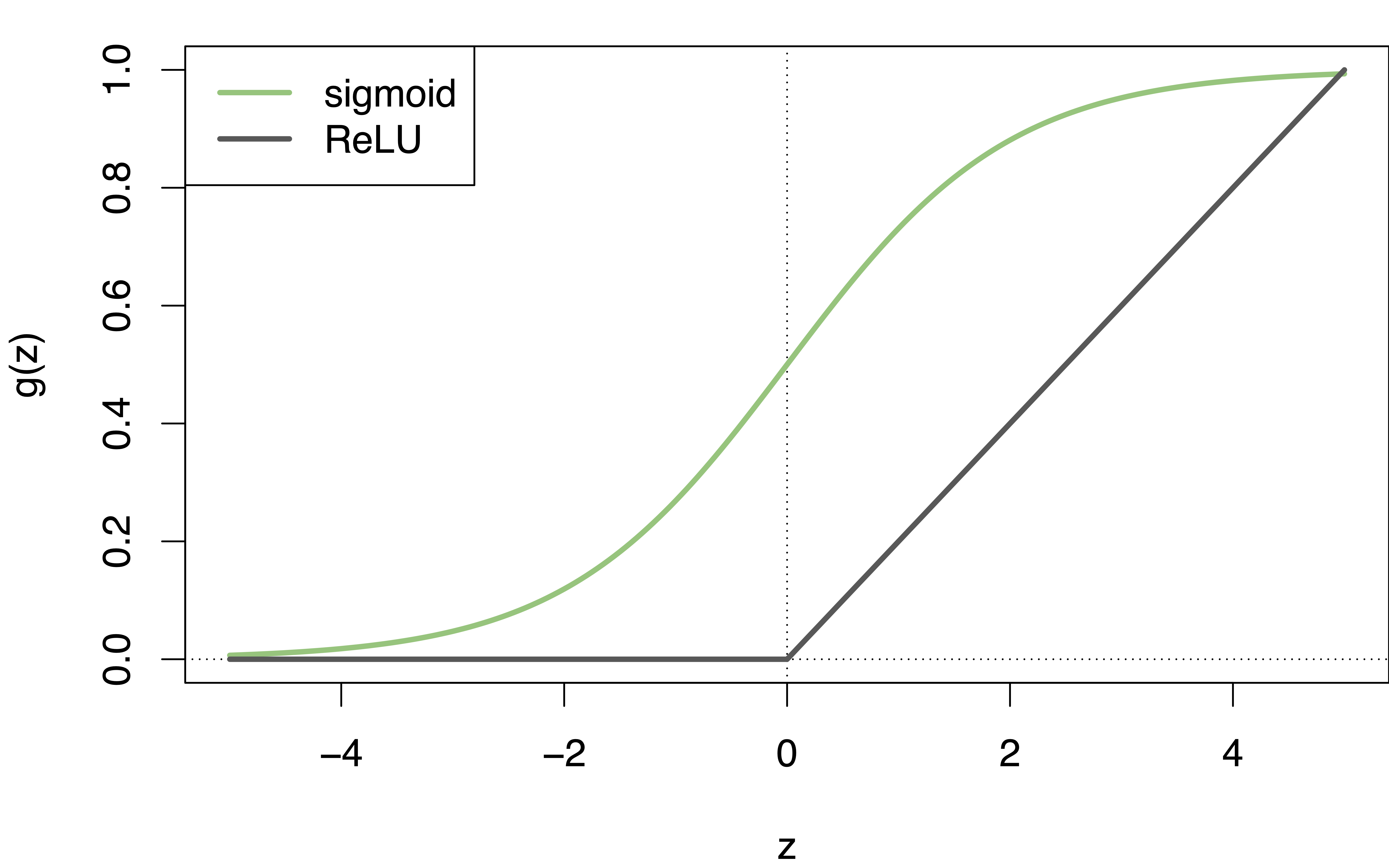
Figure 9.4: Activation Functions have non-linear shapes.

However, even though the \(g(z)\) are non-linear, the combinations in Equation 9.4 are still linear in their inputs.

The final model results from calculating linear combinations at each hidden unit, doing a non-linear transformation of each, and then, doing a linear combination on the transformed results in the final layer.
Since the final layer is still linear in its (transformed) inputs, we can use (for quantitative variables), the usual squared error loss as an objective function (loss function) to be minimized to calculate the \(\beta\)s, i.e..,

\[\sum_{i=1}^{n}(y_i - f(x_i))^2 \tag{9.7}\]

9.2.4 Learning the Weights and Biases

All of the weights \(w_{kj}\), \(biases w_{k0}\), and output weights \(\beta_k\) and \(\beta_0\) are “learned” from data.

Training typically involves defining a “loss function” for the output layer, e.g., squared error:

\[\sum_{i=1}^{n} \left( y_i - f(x_i) \right)^2\]{eq-squared-loss}

Then using gradient descent and backpropagation to adjust the weights and biases to minimize this loss.

9.2.5 Multi-layer Neural Networks

A single layer network can represent many possible \(\hat{f}(x)\).

Adding more hidden units in a layer and adding more layers allows for more possible transformations and provides more flexibility in the model.

In general, adding more, smaller layers can make solutions easier to find than just adding more units in a single layer.

Figure 9.5 shows a multi-layer network for classifying digits (0-9) with a different number of units in each hidden layer.

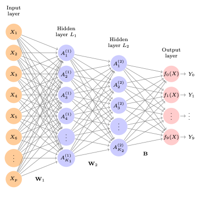
It has two hidden layers L1 (256 units) and L2 (128 units).
There are 10 nodes in the output layer since there are 10 possible levels to be classified
each is a dummy variable. In this case, the ten variables really represent a single qualitative variable so are dependent on each other.

Note

Each of the activations in the units in the second layer is still a function of the original input \(X\), albeit a transformed version of it based on the activations in the first layer.

Adding more and more layers to the model builds a series of simple transformations into a complex model for the final result.

With more layers comes more notation.

We can add a superscript to indicate the layer, e.g., \(A^{(1)}_{k}\).
Consider all the parameters for each layer as a matrix. Thus we have \(W_1\), \(W_2\) and \(B\) as our three matrices of “weights” for the network.

9.2.6 Coefficients to be Estimated

There are a lot of coefficients (weights) to be estimated in \(W_1\), \(W_2\), and \(B\).

There are 784 pixels in a \(28 \times 28\) pixel image. These are the inputs.

Matrix \(W_1\) has \(785 \times 256 = 200,960\) elements. This is based on the 256 units and the 784 input values plus the intercept term (in NN called the “bias” term).
Matrix \(W_2\) thus has \(128 \times 257 = 32,896\) (256 + bias term).
Matrix \(B\) thus has \(10 \times 129 = 1,290\) elements. The 10 linear models for each level and the 128 outputs plus the bias term.

Together there are \(200,960 + 32,896 + 1,290 = 235,146\) coefficients (weights) to be estimated.

This is 33 times more than just doing multinomial logistic regression.
With a training set of only 60,000 images, there is a lot of opportunity for overfitting.

To avoid overfitting, some regularization is needed. Options include Ridge, Lasso, or neural-network specific methods such as dropout regularization.

9.2.7 Softmax Activation Function

Since the outputs are dependent, they represent the probabilities that a given input corresponds to each possible image class and must sum to 1, this model will use the softmax activation function for the output layer.

\[f_m(X) = Pr(Y=m | X) = \frac{e^{Z_m}}{\sum_{l=0}^{9}e^{Z_l}} \tag{9.8}\]

Equation 9.8 is a generalization of the logistic function from binary logistics regression to multiple levels needed in multinomial logistic regression.

During each forward pass, the model assigns probabilities to each possible output. This is the result of the softmax “soft” prediction instead of choosing just the one value with the highest probability.
These output probabilities are a vector that sums to 1. One class may have the highest probability, but most probabilities are typically nonzero.
When training starts, probabilities are fairly evenly distributed given the random assignment of initials weights and biases. As training proceeds through multiple epochs, the model gradually shifts increases the probability for the “correct” output value and decreases other probabilities.
A key advantage of softmax is that Equation 9.8 is differentiable, which allows us to compute gradients to feed backpropagation. In contrast, the max() function is not differentiable and therefore not suitable during training.

After training is complete, when we no longer need gradients, we can apply a max() operation to the softmax output vector to make a final “hard” prediction, selecting the class (dummy variable) with the highest predicted probability as our prediction.

9.2.8 Minimization by Cross-Entropy

Since the response in this setting is qualitative (i.e., a categorical class label), we minimize the negative multinomial log-likelihood, commonly referred to as cross-entropy loss.

When class labels are represented directly as integer indices (e.g., \(y_i \in \{0, 1, \ldots, 9\}\)), the cross-entropy loss, for all \(n\) inputs, takes the form:

\[ R(\theta) = -\sum_{i=1}^{n} \log(f_{y_i}(x_i)) \tag{9.9}\]

Here, \(y_i\) is the index of the true class label for the \(i^\text{th}\) input.
\(f_{y_i}(x_i)\) is the predicted probability (from the softmax output in Equation 9.8) corresponding to that true class.

This form is computationally efficient and is the one typically used in practical implementations.

Alternatively, theoretical discussion of cross-entropy may express cross-entropy using a “one-hot encoding” of the target vector:

\[ R(\theta) = -\sum_{i=1}^{n}\sum_{m=0}^{9} y_{im} \log(f_m(x_i)) \tag{9.10}\]

Here, \(y_{im} = 1\) if class \(m\) is the correct label for input \(i\), and 0 otherwise.
\(f_m(x_i)\) is the predicted probability for class \(m\).

Equation 9.10 is mathematically equivalent to Equation 9.9 when \(y_{im}\) is one-hot encoded, and is often used to conceptually explain cross-entropy as a comparison between two distributions.

Entropy (from information theory) measures the amount of “uncertainty” or “surprise” in a probability distribution. For a predicted distribution \(p=f(X_i)\) (from our softmax output), the entropy is:

\[H(p) = -\sum_{m=0}^9 p_m \log(p_m) \tag{9.11}\]

A nearly uniform prediction (e.g., \([0.1, 0.1, ..., 0.1]\)) has high entropy (like at the end of the first epoch of training).
A perfectly confident prediction (e.g., \([0, 0, 1, 0, ..., 0]\)) has low entropy.
After the selected number of epochs, the entropy in the predicted distribution should be lower than when it started as the probabilities increase for the more-correct values and decrease for others.

Cross-entropy compares two distributions:

The true distribution \(y_i\) and
The predicted distribution \(f(x_i)\).

It is defined as:

\[H(y_i, f(x_i)) = -\sum_{m} y_{im} \log(f_m(x_i)) \tag{9.12}\]

When \(y_{im}\) is a one-hot vector, this reduces to just \(-\log(f_{m}(x_i))\), where \(m\) is the true class.
In practice, the indexed form of the loss (as in Equation 9.9) is used because it’s faster and avoids explicit one-hot encoding which takes time and memory with all the 0s.

Cross-entropy is useful in conjunction with Softmax as it is an efficient way to penalize the model more heavily when it assigns a low probability to the true class.

9.3 Fitting a Neural Network

Fitting a neural network is complex due to the necessarily non-linear activation functions.

Warning

Deep learning and neural networks is an active area of research across many communities. You will see many different terms often describing the same concept or approach.

You will also see many articles or references describing the latest approaches.

What follows is not exhaustive by any means. It is designed to provide familiarity with some approaches to provide a basic understanding.

There are many tuning (hyper-parameters) in neural networks and the selection for a given set of data is still very much an art more than a science.

While the objective function in Equation 9.7 looks familiar, minimizing it over the activation functions is non-linear.

Important

Neural Networks use non-linear activation functions so their objective functions are non-convex and have multiple local optima in addition to a global optimum.

Instead of trying to find the “best” model at the one global optimum, potentially out of millions, we seek to find a useful model at a “reasonable” local minima.

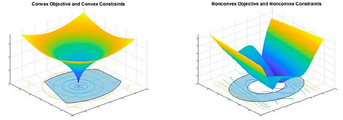
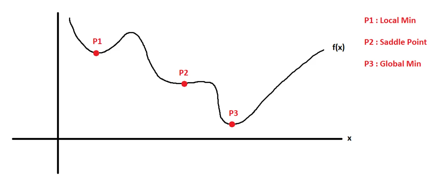
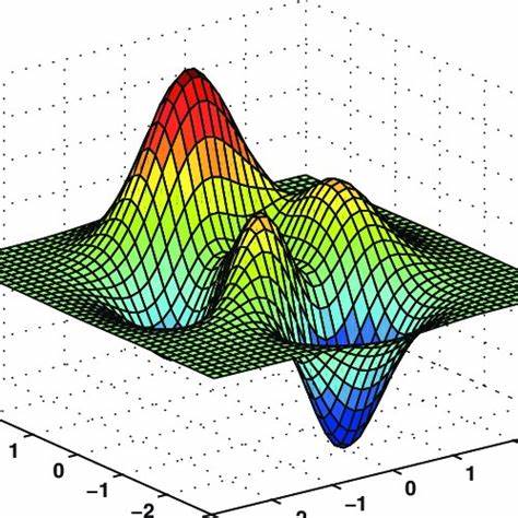
Two strategies help find better local optima and reduce the chance of overfitting.

Slow Learning: slow learning uses small steps to reduce the chance of overfitting. The algorithm stops when overfitting is detected.
Regularization: Imposing penalties on the parameters such as with Ridge and LASSO regression.

Assume all the parameters (coefficients) are in a single vector \(\theta\).

Define the objective then as

\[R(\theta) = \frac{1}{2}\sum_{i=1}^n(y_i - f_\theta(x_i))^2. \tag{9.13}\]

General Algorithm to Minimize the Objective Function

To find the best parameters \(\theta\) for our model, we want to minimize the objective function:

\[R(\theta) = \frac{1}{2} \sum_{i} (y_i - f_\theta(x_i))^2\]

A general optimization algorithm could look like this:

Initialize: Make an initial guess for all the parameters, \(\theta^0\), and set \(t = 0.\)
Update step: Find a vector \(\delta\) that represents a small change in \(\theta\)such that the new parameters \(\theta^{t+1} = \theta^t + \delta\) reduce the value of \(R(\theta^t)\).
Check improvement: If \(R(\theta^{t+1}) < R(\theta^t)\), set \(t = t + 1\) and return to step 2.
Stop condition: If no meaningful reduction is achieved, stop. The algorithm has likely reached a local minimum of the loss function.

How do we find a good \(\delta?\)

9.3.1 Gradient Descent and Backpropagation

Finding \(\delta\) is the core challenge in training neural networks.

We want to move \(\theta\) in the direction that reduces the error most efficiently.
That direction is given by the negative of the gradient of the objective function: \(\delta = -\eta \cdot \nabla_\theta R(\theta)\)

Note

Think of the gradient as a slope of a line but in multiple dimensions, the default calculation points in the direction of steepest increase in the loss.

So, to minimize the loss, we move in the opposite direction of the gradient - the negative gradient.

Imagine you are on a hill and want to get to the valley below (reach the lowest point (the minimum loss)).

The gradient is the direction the hill is steepest.
If you step in the opposite direction of the gradient, you’re going downhill and finding the better set of weights and bias that will give you a lower error.
The learning rate is how big of a step you take before you calculate the next gradient.

Each weight and bias has its own gradient — we update them individually using a method called gradient descent.

The gradient, \(\nabla_\theta R(\theta)\), shows how the error would change by updating (increasing or decreasing) each weight/bias.
The learning rate, \(\eta\) (eta) controls how big a step we take in the opposite direction of the gradient.
The minus sign ensures we move in the direction that reduces the error, not increases it.
You may see the term the “gradient vector” for a node which is shorthand for the set of all the individual gradient entries for each weight/bias parameter.

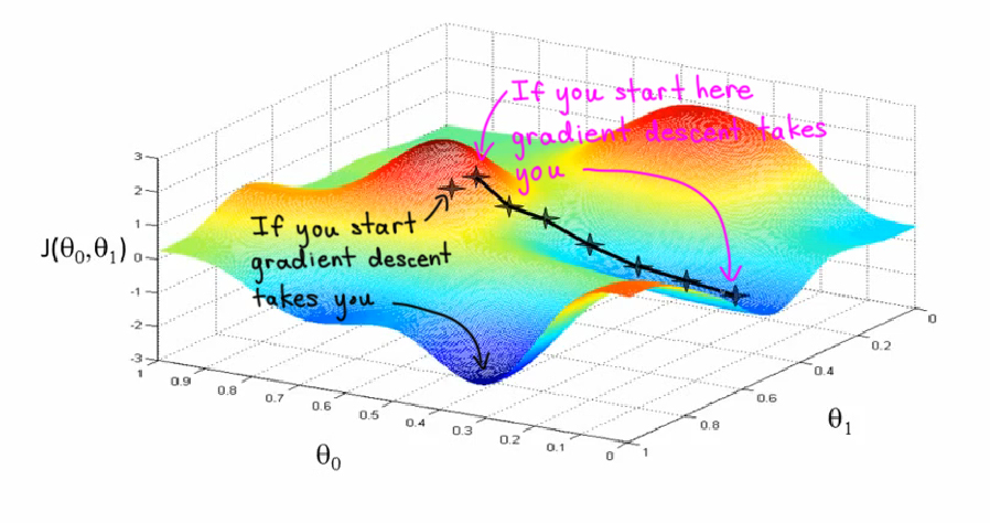
Figure 9.7 provides one view of how gradient descent can lead to different local optima with slightly different starting points.

Figure 9.7: Conceptual view of Gradient Descent (Rashida048 (2020))

9.3.1.1 Backpropagation: An Intuitive Analogy

Backpropagation is how a neural network learns from its mistakes. You can think of it like how a child learns to shoot a basketball:

Take a shot: The child throws the ball — this is the network making a prediction.
See the result: The child sees if the shot missed or scored — this is the model calculating the error.
Figure out what went wrong: Did the shot go too far? Was the angle off? — this is feedback.
Adjust next time: The child throws again, tweaking their motion — this is weight adjustment using backpropagation.

How It Works in a Neural Network

The prediction is the forward pass — the model computes \(f_\theta(x)\).
The error is the difference between predicted and actual values: \(y_i - f_\theta(x_i)\).
Backpropagation takes this final error and sends it backward through the network, using the chain rule as it goes layer by layer, to calculate the gradient of the loss with respect to every weight/bias parameter.

In other words:

Starting with the residual (final error), we compute how much each parameter contributed to that error and how it should change.

This is done layer-by-layer from right to left (going backwards, output to input), updating weights across each layer.

9.3.1.2 Why It Matters

Backpropagation makes training deep models computationally feasible. It allows the model to:

Efficiently compute \(\nabla_\theta R(\theta)\) for all parameters, even in deep networks.
Update its parameters using a simple rule: \(\theta^{t+1} = \theta^t - \eta \cdot \nabla_\theta R(\theta^t)\)
Learn from experience, gradually reducing error as it sees more examples.

9.3.2 Epochs

We know how to do three things:

A Forward Pass: Use the initial inputs to compute the outputs for each unit in each layer (using the estimated weights and activation functions) to get to an output layer where the parameters (\(\beta\)s) are estimated (based on optimizing a loss function) to produce a prediction \(\hat{y}_i\) for each observation \(x_i\).
Calculate the residuals \((\hat{y}_i - y_i)\).
A Backwards Pass: Use the gradient of the loss function to allocate the residuals as a \(\delta\) to update each of the weights in the network thorough backpropagation.

We will repeat those steps multiple times in training the network.

An Epoch is defined as one complete forward pass and a complete backward pass (steps 1-3) through the network where every observation in the training data set contributes to the update.

The number of epochs to use is a tuning parameter when building the model.
There are trade offs of time and accuracy as well preventing overfitting.

9.3.3 Options for Epochs

With so many calculations to be made, there are different approaches to how to use the training data in each epoch.

Massive data sets can require many computations and significant memory to hold all the data at once.
Research continues into multiple options for improving the speed and reducing the memory requirements for neural networks.

Each approach has trade offs between how long it takes to complete an epoch, how fast or slow to get to convergence, how smoothly to get to convergence, how to reduce bias or multicollinearity, and how much memory is required.

There are three popular approaches for how much data to include in each forward/backward pass through the network. see Batch, Mini Batch & Stochastic Gradient Descent.

Batch Gradient Descent
- All the observations are used at once, in a single batch or iteration.
- When data space is “well-behaved”, it can provide for a smooth convergence across multiple epochs.
- It does require all the data fit into memory at once.
Stochastic Gradient Descent is the other extreme where only one observation at a time is fed into the model.
- Thus there are \(n\) batches and each batch is processed in an iteration.
- Much less data has to be computed each time and much less has to fit into memory.
- The convergence can be less smooth as observations can vary widely.
Mini-Batch Gradient Descent
- This is in between the others where a fraction of the data is used for each batch.
- If there are \(m\) batches, each batch uses \(n/m\) observations with the last batch using whatever remains after the \(m-1\)^st batch.
- There are different methods for whether to update the \(\delta\)s after each mini-batch (do a backwards pass) or just store the residuals from a forward pass to update \(\delta\)s after all mini-batches have been run and you have \(n\) residuals.
- There is some evidence that small batches (32) may be less smooth but converge more quickly and be more robust in prediction.
Hybrid Approaches
- This is my term for the variety of methods that combine aspects of multiple approaches.
- One such method is to select the observations for each iteration at random (with/without replacement.
- This would mean that perhaps not all \(n\) observations made it into each epoch.
- Another method is to randomly shuffle all the input data at each epoch so different data goes into different batches for each epoch.

Note

Some use the term Stochastic Gradient Descent (SGD) as shorthand to refer to all the above approaches for selecting the data to be used in an iteration.

Since the number of coefficients to be estimated (the \(w\)s and \(\beta\)s) can often be greater than the number of observations, using a regularization method can reduce the risk of overfitting.

9.4 Regularization of Neural Networks

9.4.1 Regularization Methods for Optimization.

We could use Ridge or LASSO Regression.

For Ridge, we add the Ridge penalty term (i.e., L2 regularization) to Equation 9.9 to now optimize

\[ R(\theta; \lambda) = -\sum_{i=1}^{n} \log(f_{y_i}(x_i)) + \lambda \sum_j \theta_j^2 \tag{9.14}\]

The first term is the negative log-likelihood or cross-entropy loss based on the true class label \(y_i\) and its predicted probability \(f_{y_i}(x_i)\).
The second term is the Ridge penalty, which discourages large weights in the model and helps prevent overfitting.
The sum \(\sum_j \theta_j^2\) typically runs over all model parameters \(\theta_j\), possibly excluding bias terms, depending on implementation.

For LASSO, we would change the last term to the absolute value \(L_1\) norm or \(\lambda\sum_j|\theta_j|\).

We can set \(\lambda\) to a small value or use a validation method to get it.
We could choose separate values of \(\lambda\) for each layer as well.

We could also implement a hyper-parameter to “stop early” to reduce overfitting.

9.4.2 Dropout Learning

Dropout Learning is a regularization method similar to Random Forests where for each iteration in an epoch, we randomly select a fraction of the nodes, \(\phi\), to “drop out” of the calculation.

The remaining weights are scaled by a factor of \(1/(1-\phi)\) to compensate for the missing units.
In practice, dropout is achieved by randomly setting the activations for the “dropped out” units to zero.

One can also insert a “dropout layer” between the input nodes and the first hidden layer.

Dropout Learning reduces the opportunity for nodes to become “too specialized” as other nodes have to make up for the residuals when they are dropped out. This tends to improve performance in prediction.

There are multiple suggestions to help with adjusting the drop out rate (Dropout Regularization in Deep Learning Models with Keras). These include:

Use a small dropout value of 20%-50% of neurons, with 20% providing a good starting point. A probability too low has minimal effect, and a value too high results in under-learning by the network.
Use a larger network. You are likely to get better performance when Dropout is used on a larger network, giving the model more of an opportunity to learn independent representations.
Use Dropout on incoming (visible) as well as hidden units. Application of Dropout at each layer of the network has shown good results.

9.5 Tuning Neural Networks

Tuning a Neural Network has additional complexity beyond selecting the inputs.

The model developer has to choose:

Designing the network based on the number of hidden layers, and the number of units per layer.
Setting the parameters for stochastic gradient descent. These includes the batch size, the number of epochs, and if used, details of data augmentation
Regularization tuning parameters depending upon the method(s) in use. These include the size of \(\lambda\) for Ridge or LASSO for each layer as well as the dropout fraction \(\phi\).

It is common to plot the improvement in model performance against the number of epochs to see if there is a good stopping point.

If the improvement is too rough/noisy, you can shrink the learning rate to smooth things out.

Properly tuned networks can take some time. However, they can outperform other methods.

9.6 Example of Deep Learning in R

We will use the hitters database from {ISLR2}.(James et al. 2023)

Let’s predict Salary based on all the other predictors and calculate the mean absolute prediction error.

We will use Tensorflow and Keras and which are popular open-source platforms for doing machine learning using Python.

TensorFlow is an end-to-end platform for machine learning.
A tensor is a specific class of a data structure similar to a matrix or python numpy array.
The tensor “flows” through the network model as each iteration completes a forward and then a backwards pass.
TensorFlow typically requires tensors to be “rectangular”, that is, the elements on each axis must be the same size.
There are specialized types of tensors that can handle different shapes.
Keras is a high-level API built on top of TensorFlow.
You use Keras to define the architecture of your neural network (layers, nodes ,etc.), while TensorFlow handles the underlying computations.

We can access TensorFlow and Keras in R by using the {reticulate} package (Ushey, Allaire, and Tang 2023) and specific packages for each.

9.6.1 Python - TensorFlow - Keras Setup

Setup can take some time to configure properly depending upon what you already have installed on your system.

See the following references for assistance in installing {reticulate}, a version of python, {tensorflow}, and {keras}.

The following maybe helpful for the first time install on a local machine.

reticulate::install_miniconda(force = TRUE)
reticulate::use_miniconda()  # sets up the path to miniconda
reticulate::miniconda_path() # Should be ~/Library/r-miniconda on macOS
# C:/Users/<your-username>/AppData/Local/r-miniconda on windows

reticulate::py_config() # confirm the setup
reticulate::virtualenv_create(envname = "r-reticulate")

# install.packages("remotes")
remotes::install_github("rstudio/tensorflow")
library(tensorflow)
# For Non-Mac silicon
install_tensorflow(version = "2.16.2", envname = "r-tensorflow")

#For Mac Silicon (no NVIDIA GPUs)
reticulate::conda_create("r-tf-macos", python_version = "3.9")
reticulate::conda_install("r-tf-macos", packages = c("tensorflow-macos", "tensorflow-metal"), pip = TRUE)
reticulate::use_condaenv("r-tf-macos", required = TRUE)
Sys.unsetenv("RETICULATE_PYTHON")
reticulate::use_python("/Users/rressler/Library/r-miniconda-arm64/envs/r-tf-macos/bin/python")

Important

Although silicon Mac machines have Graphical Processing Units (GPUs), they are not compatible with the TensorFlow set up. Thus the commands above can help you install a version of TensorFlow for the Mac OS to use CPUs instead, which can be slower.

9.6.2 Prepare the data

Remove NAs and set up a vector for making a test set of 1/3 the observations.

library(ISLR2)
Gitters <- na.omit(Hitters)
dplyr::glimpse(Gitters)

Rows: 263
Columns: 20
$ AtBat     <int> 315, 479, 496, 321, 594, 185, 298, 323, 401, 574, 202, 418, …
$ Hits      <int> 81, 130, 141, 87, 169, 37, 73, 81, 92, 159, 53, 113, 60, 43,…
$ HmRun     <int> 7, 18, 20, 10, 4, 1, 0, 6, 17, 21, 4, 13, 0, 7, 20, 2, 8, 16…
$ Runs      <int> 24, 66, 65, 39, 74, 23, 24, 26, 49, 107, 31, 48, 30, 29, 89,…
$ RBI       <int> 38, 72, 78, 42, 51, 8, 24, 32, 66, 75, 26, 61, 11, 27, 75, 8…
$ Walks     <int> 39, 76, 37, 30, 35, 21, 7, 8, 65, 59, 27, 47, 22, 30, 73, 15…
$ Years     <int> 14, 3, 11, 2, 11, 2, 3, 2, 13, 10, 9, 4, 6, 13, 15, 5, 8, 1,…
$ CAtBat    <int> 3449, 1624, 5628, 396, 4408, 214, 509, 341, 5206, 4631, 1876…
$ CHits     <int> 835, 457, 1575, 101, 1133, 42, 108, 86, 1332, 1300, 467, 392…
$ CHmRun    <int> 69, 63, 225, 12, 19, 1, 0, 6, 253, 90, 15, 41, 4, 36, 177, 5…
$ CRuns     <int> 321, 224, 828, 48, 501, 30, 41, 32, 784, 702, 192, 205, 309,…
$ CRBI      <int> 414, 266, 838, 46, 336, 9, 37, 34, 890, 504, 186, 204, 103, …
$ CWalks    <int> 375, 263, 354, 33, 194, 24, 12, 8, 866, 488, 161, 203, 207, …
$ League    <fct> N, A, N, N, A, N, A, N, A, A, N, N, A, N, N, A, N, N, A, N, …
$ Division  <fct> W, W, E, E, W, E, W, W, E, E, W, E, E, E, W, W, W, E, W, W, …
$ PutOuts   <int> 632, 880, 200, 805, 282, 76, 121, 143, 0, 238, 304, 211, 121…
$ Assists   <int> 43, 82, 11, 40, 421, 127, 283, 290, 0, 445, 45, 11, 151, 45,…
$ Errors    <int> 10, 14, 3, 4, 25, 7, 9, 19, 0, 22, 11, 7, 6, 8, 10, 16, 2, 5…
$ Salary    <dbl> 475.000, 480.000, 500.000, 91.500, 750.000, 70.000, 100.000,…
$ NewLeague <fct> N, A, N, N, A, A, A, N, A, A, N, N, A, N, N, A, N, N, N, N, …

n <- nrow(Gitters)
set.seed(13)
ntest <- trunc(n / 3)
testid <- sample(1:n, ntest)

9.6.3 Prepare Models using Other Methods for Comparison

Create a linear model as a basis for comparison.

lfit <- lm(Salary ~ ., data = Gitters[-testid, ])
lpred <- predict(lfit, Gitters[testid, ])
lae_lm <- with(Gitters[testid, ], mean(abs(lpred - Salary)))
lae_lm

[1] 254.6687

Let’s create a LASSO model as a basis for comparison.

Create the model matrix from the linear model and scale it for use in cv.glm().
Run cv.glm() using type-measuer="mae" and then calculate the mean absolute prediction error.
The {glmnet} package includes cv.glm() which uses Cross-Validation to measure predictive error so you do not need to use a validation set.

x <- scale(model.matrix(Salary ~ . - 1, data = Gitters))
y <- Gitters$Salary

library(glmnet)
set.seed(123)
cvfit <- cv.glmnet(x[-testid, ], y[-testid], type.measure = "mae")
cpred <- predict(cvfit, x[testid, ], s = "lambda.min")
lae_lasso <- mean(abs(y[testid] - cpred))
lae_lasso

[1] 253.1462

Slightly better.

9.6.4 Set up the Network Model

First we have to define the neural network object as a sequential learning model.

Load the {keras3} package with library().
- We use {keras3} to define our network and set several hyper-parameters.
- It is part of the TensorFlow framework.
keras_model_sequential creates a model object in which we can define a “stack of layers”.
- A sequential model is appropriate for a plain stack of layers where each layer has exactly one input tensor and one output tensor.
- This includes both the single hidden layer model and the multiple hidden layer models discussed earlier.
Specify each layer in order using layer_dense().
- Here we define a single hidden layer with 50 units and the ReLU activation function.
You can also set the dropout layer with layer_dropout().
- Here we set a dropout rate of .4 or 40% of the activations from the previous layer will be set to 0 each pass.
Finally, add the last layer (the output).
- Here we want only one prediction, so one unit with no activation function.

Important

For newer models install {keras3} and then keras3::install_keras() to be in sync with the updated {tensorflow} package.

See https://github.com/rstudio/keras3/issues/1428

library(keras3)

# Create the model
my_model <- keras_model_sequential()
# Add layers to the model
layer_dense( object = my_model, 
               units = 50, activation = "relu", input_shape = ncol(x)) |> 
  layer_dropout(rate = 0.4) |> 
  layer_dense(units = 1) ->
  my_model

# Print model summary
summary(my_model)

Model: "sequential"
┏━━━━━━━━━━━━━━━━━━━━━━━━━━━━━━━━━━━┳━━━━━━━━━━━━━━━━━━━━━━━━━━┳━━━━━━━━━━━━━━━┓
┃ Layer (type)                      ┃ Output Shape             ┃       Param # ┃
┡━━━━━━━━━━━━━━━━━━━━━━━━━━━━━━━━━━━╇━━━━━━━━━━━━━━━━━━━━━━━━━━╇━━━━━━━━━━━━━━━┩
│ dense (Dense)                     │ (None, 50)               │         1,050 │
├───────────────────────────────────┼──────────────────────────┼───────────────┤
│ dropout (Dropout)                 │ (None, 50)               │             0 │
├───────────────────────────────────┼──────────────────────────┼───────────────┤
│ dense_1 (Dense)                   │ (None, 1)                │            51 │
└───────────────────────────────────┴──────────────────────────┴───────────────┘
 Total params: 1,101 (4.30 KB)
 Trainable params: 1,101 (4.30 KB)
 Non-trainable params: 0 (0.00 B)

Now that we have built the model for training, we have to get it into a structure to tell the python engine about it.

compile() invokes compile.keras.engine.training.Model ()
We have to tell it the optimizer to use. For most models that is optimizer_rmsprop().
We also have to tell it the metrics to be evaluated by the model during training and testing.
By default, Keras will create a placeholder for the model’s target “tensor” (input data), which will be fed with the target data during training.

my_model |> 
  compile(loss = "mse",
    optimizer = optimizer_rmsprop(),
    metrics = list("mean_absolute_error")
   )

9.6.5 Fit the Neural Network Model

Now we fit the model.

fit() invokes fit.keras.engine.training().
We supply the training data and two fitting parameters, epochs and batch_size.
Using a batch of 32 at each step of descent, the algorithm selects 32 training observations for the computation of the gradient.
Let’s start with just 15 epochs.
We also use the testing data for the validation_data= argument.

history <- my_model |> 
  fit(
#    x[-testid, ], y[-testid], epochs = 750, batch_size = 32, verbose = 0,
    x[-testid, ], y[-testid], epochs = 15, batch_size = 32,
    validation_data = list(x[testid, ], y[testid])
  )

Epoch 1/15
6/6 - 0s - 59ms/step - loss: 456996.9688 - mean_absolute_error: 533.7785 - val_loss: 556016.0625 - val_mean_absolute_error: 539.7103
Epoch 2/15
6/6 - 0s - 6ms/step - loss: 456686.5938 - mean_absolute_error: 533.4979 - val_loss: 555649.3750 - val_mean_absolute_error: 539.4686
Epoch 3/15
6/6 - 0s - 6ms/step - loss: 456313.3125 - mean_absolute_error: 533.1774 - val_loss: 555354.0000 - val_mean_absolute_error: 539.2758
Epoch 4/15
6/6 - 0s - 6ms/step - loss: 456054.4688 - mean_absolute_error: 532.9685 - val_loss: 555044.1250 - val_mean_absolute_error: 539.0750
Epoch 5/15
6/6 - 0s - 6ms/step - loss: 455670.6250 - mean_absolute_error: 532.7266 - val_loss: 554748.0625 - val_mean_absolute_error: 538.8831
Epoch 6/15
6/6 - 0s - 6ms/step - loss: 455357.7812 - mean_absolute_error: 532.4951 - val_loss: 554429.5625 - val_mean_absolute_error: 538.6810
Epoch 7/15
6/6 - 0s - 6ms/step - loss: 455373.5312 - mean_absolute_error: 532.3773 - val_loss: 554096.6875 - val_mean_absolute_error: 538.4705
Epoch 8/15
6/6 - 0s - 6ms/step - loss: 454967.5938 - mean_absolute_error: 532.0938 - val_loss: 553785.3125 - val_mean_absolute_error: 538.2706
Epoch 9/15
6/6 - 0s - 6ms/step - loss: 454728.9688 - mean_absolute_error: 531.9525 - val_loss: 553453.3125 - val_mean_absolute_error: 538.0537
Epoch 10/15
6/6 - 0s - 6ms/step - loss: 454156.2812 - mean_absolute_error: 531.5709 - val_loss: 553094.8750 - val_mean_absolute_error: 537.8401
Epoch 11/15
6/6 - 0s - 6ms/step - loss: 454097.6250 - mean_absolute_error: 531.5056 - val_loss: 552764.0625 - val_mean_absolute_error: 537.6342
Epoch 12/15
6/6 - 0s - 6ms/step - loss: 453749.1875 - mean_absolute_error: 531.2587 - val_loss: 552390.1250 - val_mean_absolute_error: 537.4103
Epoch 13/15
6/6 - 0s - 6ms/step - loss: 453439.3750 - mean_absolute_error: 530.9985 - val_loss: 552037.2500 - val_mean_absolute_error: 537.1979
Epoch 14/15
6/6 - 0s - 6ms/step - loss: 452984.4688 - mean_absolute_error: 530.7775 - val_loss: 551648.1250 - val_mean_absolute_error: 536.9709
Epoch 15/15
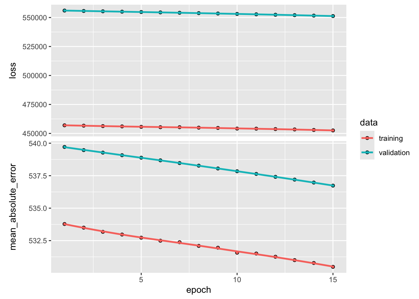
6/6 - 0s - 6ms/step - loss: 452580.6875 - mean_absolute_error: 530.4810 - val_loss: 551256.8125 - val_mean_absolute_error: 536.7348

class(history)

[1] "keras_training_history"

We can plot the results for the most recent set of epochs.

It uses {ggplot2} if available by default, otherwise Base R graphics.
There are plotting options for plot.keras_training_history() but it is not exported from {keras}.
You can look at help, but not call it directly.

plot(history)

Note

If you run the fit() command a second time in the same R session, the fitting process will pick up where it left off.

Try re-running the fit() command, and then the plot() command!
You can restart R to reset.

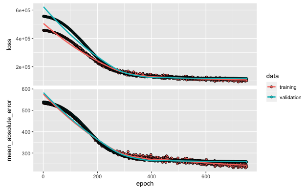
Here is an example plot for 750 epochs.

Note how the green line for the test set (validation data) starts to stay above the training data at about 500 epochs.
This can be suggestive of overfitting.

9.6.6 Predict and Measure Performance

predict() invokes predict.keras.engine.training.Model().

summary(my_model)

Model: "sequential"
┏━━━━━━━━━━━━━━━━━━━━━━━━━━━━━━━━━━━┳━━━━━━━━━━━━━━━━━━━━━━━━━━┳━━━━━━━━━━━━━━━┓
┃ Layer (type)                      ┃ Output Shape             ┃       Param # ┃
┡━━━━━━━━━━━━━━━━━━━━━━━━━━━━━━━━━━━╇━━━━━━━━━━━━━━━━━━━━━━━━━━╇━━━━━━━━━━━━━━━┩
│ dense (Dense)                     │ (None, 50)               │         1,050 │
├───────────────────────────────────┼──────────────────────────┼───────────────┤
│ dropout (Dropout)                 │ (None, 50)               │             0 │
├───────────────────────────────────┼──────────────────────────┼───────────────┤
│ dense_1 (Dense)                   │ (None, 1)                │            51 │
└───────────────────────────────────┴──────────────────────────┴───────────────┘
 Total params: 2,204 (8.61 KB)
 Trainable params: 1,101 (4.30 KB)
 Non-trainable params: 0 (0.00 B)
 Optimizer params: 1,103 (4.31 KB)

npred <- predict(my_model, x[testid, ])

3/3 - 0s - 11ms/step

mean(abs(y[testid] - npred))

[1] 536.7348

After just a few epochs, the model will probably not perform as well as the other models.
Here is one set of sequential outputs - running each set of epochs one after the other.
- 15 Epochs yields LAE of 537.4442.
- 200 yields 378.8374
- 500 yields 271.2441
- 700 yields 264.6041
- 1,000 yields 259.3959
- 1,500 yields 255.6646
- 2,000 yields 256.7299
These are all higher than the 253 achieved by the Lasso model. However, more tuning may get better results.
- One set of sequential runs had a result of 248.

Warning

Reproducing results can be a challenge in this setting as setting a seed in R does not carry over into Python where TensorFlow is running.

Keras and TensorFlow allow the building of very complicated models for a variety of purposes.

The more complicated the model the more hyper-parameters might be required and thus more dimensions to the tuning space to find the most useful model.

9.7 Convolutional Neural Networks (CNN)

Convolutional Neural Networks (CNNs) are a special type of neural network architecture designed for processing grid-like data, particularly images.

CNNs excel at tasks like image classification, object detection, and facial recognition by automatically learning features from pixel data and using them to make accurate predictions.

Figure 9.8 shows a typical CNN such as might be used for image classification (cat or dog).

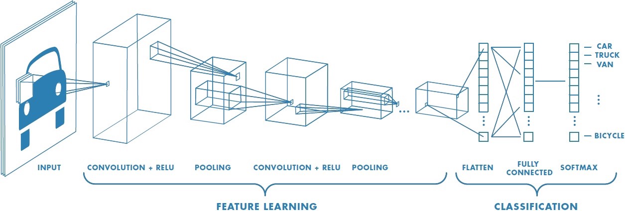
On the left of Figure 9.8 is the Input Layer: Raw Pixel Data

Every CNN begins with an input layer that takes in the image as a multi-dimensional array of pixel values. For a color image, this typically includes three channels—red, green, and blue—resulting in a 3D input tensor (height × width × channels). The numerical values represent the intensity of each pixel.

Convolutional Layers: Feature Detectors

The first major component of a CNN is a convolutional layer of which there can be several.

This layer applies small, trainable filters (“kernels”) that scan across the image to detect patterns.
Each convolutional kernel (filter) performs an element-wise multiplication between the filter’s weights and a small patch of the input (e.g., a 3×3 section of pixels).
- The resulting values are summed to produce a single number, which becomes one pixel in the feature map.
  - The filter then slides (or convolves) one pixel to the right (this is called the stride), and repeats the process across the width of the input.
  - After completing one row, it slides down one pixel and starts again at the left.
  - This continues until the filter has covered the entire image, producing a feature map as a 2D grid where each value represents the presence of a learned pattern at that location.

Key properties:

Local connectivity: Filters examine local regions, preserving spatial relationships.
Weight sharing: Each filter uses the same weights across the image, reducing model complexity.
Depth: Multiple filters can be applied in a single convolutional layer, capturing various patterns simultaneously.

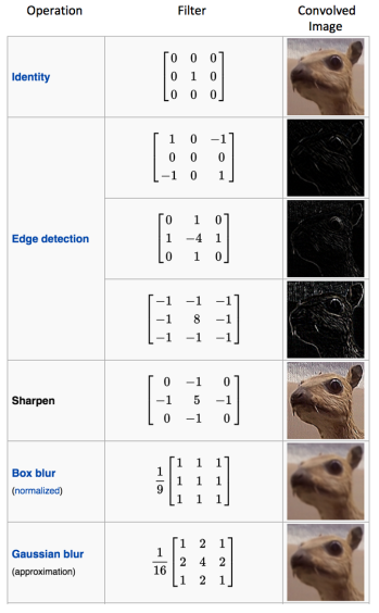
Early convolutional layers detect simple features like edges or colors; deeper layers detect more abstract concepts like shapes or object parts as shown in Figure 9.9.

Figure 9.9: Sample Convolution Operations and Filters

Activation Function: Non-Linearity

After each convolution operation, an activation function, usually ReLU, is to introduce non-linearity by zeroing out negative values:

This allows the network to model complex patterns and relationships that simple linear transformations cannot.

Pooling Layers: Spatial Reducers

Next come pooling layers, which reduce the spatial dimensions of the feature maps.

The most common pooling operation is “max pooling”, which slides a small window (e.g., 2×2) over the feature map and takes the maximum value in each region. This step simplifies the data, makes the network more computationally efficient, and introduces a level of translation invariance.

Key benefits:

Reduces the number of parameters.
Controls overfitting.
Preserves the most important features while discarding minor variations.

Pooling doesn’t alter the number of feature maps; it just compresses them.

Stacking Layers for Hierarchical Feature Learning

CNNs often stack multiple convolutional and pooling layers to learn a hierarchy of features as in Figure 9.8:

Shallow layers detect low-level features like edges and corners.
Intermediate layers detect textures, patterns, and shapes.
Deep layers capture high-level features and object parts.

This layered approach is what gives CNNs their strength in capturing complex patterns in images.

Fully Connected Layers: Classification

After the final convolutional and pooling layers, the high-level feature maps are flattened into a single vector and passed into one or more fully connected layers. These layers act like a traditional neural network, using the learned features to predict a class label or probability distribution over multiple categories (e.g., Dog, Cat, Tiger, Lion).

Output Layer

The final layer is often a softmax classifier (for multi-class classification), which outputs a probability score for each class. The highest score determines the predicted category of the image.

Note

Kernels in CNNs vs. SVMs

It’s important to note that kernels in CNNs are not the same as kernels in Support Vector Machines (SVMs):

CNN kernels are learnable filters used to detect spatial patterns directly from input data.
SVM kernels are mathematical functions (like polynomial) used to project data into higher-dimensional spaces to find separating boundaries.

While they share a name, they serve entirely different purposes in their respective algorithms.

CNNs are powerful because they combine:

Local feature detection (via convolution),
Efficient dimensionality reduction (via pooling),
Non-linear transformations (via activation functions),
and final classification (via fully connected layers).

This architecture allows them to automatically learn meaningful features and make accurate predictions from raw image data—without the need for manual feature engineering.

9.8 Summary

Important

Deep Learning and Neural Networks is a vast field of research and application.

There are multiple variants for working with special classes of problems such as Convolutional Neural Networks, or building models upon model or models that compete with other models.

While Deep Learning and Neural Networks can be a powerful method for prediction, it often of little help in inference as the models tend to be “black-box” models where explainability is hard.

Deep Learning and Neural Networks may also dominated by other methods depending upon the data set and question to be answered. Once one considers constraints on the available resources in computational power/memory as well as the time it takes to properly tune a model for maximum performance, other methods much better choices if they perform reasonably well.

To reduce some of that time and expense, consider using pre-trained models for your use case, such as on Hugging Face and tune it to your specific needs. Or you could start with a pre-trained model and use Fine Tuning to customize to your domain. Finally, you could consider building a Retrieval Augmented Generation (RAG) architecture model to customize an existing Large Language Model to better work in your domain.

Machines may learn, but humans still need to know how to make choices to generate useful results.