2  Cleaning and Reshaping Data

Keywords

data wrangling, dplyr, tidyr, stringr, regex, joins

2.1 Introduction

This module focuses on step 4 in the life cycle- Shape Data. It introduces some core data science skills in cleaning and shaping data - it’s what data scientists do.

Learning Outcomes

• Explain the need to clean data.
• Clean and shape rectangular data: filter rows, select columns, rename columns, …
• Explain basic methods for reshaping and combining data: pivots and joins.

2.1.1 References

These are all core {tidyverse} packages:

• Manipulating Data Frames: {dplyr} package (Wickham et al. 2023)
• Manipulating String or Character Data: {stringr} package (Wickham 2023c)
• Manipulating Dates and Time Data:{lubridate} package (Grolemund and Wickham 2011)
• Manipulating Factor or Categorical Data:{forcats} package (Wickham 2023a)
• Reshaping Data Frames: {tidyr} package (Wickham, Vaughan, and Girlich 2023)

Other References

• Cleaning Data Frames: {janitor} package (Firke 2024)

2.2 Cleaning Data

Once we have a question, framed the analysis, and found some data, it is time for step 4 in the life cycle - cleaning and shaping the data so it can be used for analysis.

2.2.1 Real Data is Messy

Data from formal research experiments with randomized trials is usually well-designed to support the analytical approach. (Thank your statistician friends!)

• There can still be measurement errors, input errors (Female, Femmale, Fem, 1, Woman), sampling errors, multiple ways of indicating NA (na, -999, null) or duplication.

However, most data is “observational”, created for purposes other than your analysis.

• Even with the growth of the Internet of Things (IOT) devices generating data, humans still create more data than devices, and most of that data is text.

Observational real-world data is usually messy. In addition to the errors in “good” experimental data, …

• It is often incomplete, so not every variable is present that you might want.
• Humans are “notorious” for their creativity when using text - it is a feature and a bug.
• Even when entering numeric data, we make mistakes such as switching numbers, adding spaces, putting the decimal point in the wrong place, ….
• Most data is designed for humans to read and not for computers to analyze.
• Real-world data is often missing values, has different formats (e.g., times and dates).
• When data is scraped from web pages or PDFs there are often random errors in it.
• Tabular data in customized tables with merged rows or columns can be hard to parse correctly.

Given the vast amount of messy data, there are multiple names to describe what happens in cleaning and shaping data. These include

1. Data “wrangling”: The overall process of cleaning, transforming, and preparing raw data for analysis.
2. Data “munging”: Informal synonym for data wrangling; often used to describe converting messy or unstructured data into a usable format.
3. Data pre-processing: Steps taken before actual analysis, such as handling missing values, encoding categories, and scaling.
4. Feature engineering: Creating new variables (features) or modifying existing ones to improve the performance of models.
5. Data normalization: Transforming data to a common scale without distorting differences in the ranges of values (e.g., min-max scaling or z-score standardization).

Regardless of the name, the steps of getting the data and then preparing it for analysis often take much longer than and require as much creativity as building a model or running statistical tests.

Surveys support the idea that many data scientist spend between 40% to 80% of the time on a project working to get data, clean it, and shape it.

• This is often an iterative process as you try some data and then realize you need more.

2.3 Rectangular and Tidy Data

The goal for cleaning and shaping data is use a reproducible process to get the data in its most accurate and consistent representation in a format that is easy to use in analyzing the question of interest.

• We want reproducible process so we can more easily update the data if new data arrives, say a new month or year of data is released.
• We want the data to be accurate and consistent so we minimize noise in our analysis.
• We want the data in an easy to use format so we can apply standard methods and tool.

Starting with the format, we want our data in rectangular format known as a data frame.

• R, Python and Excel all work best with rectangular data: a table where the rows are the multiple observations (records) for an entity and the columns are the attributes of the entity which we refer to as variables.

In R, a data frame has class data.frame and the tidyverse works with a special kind of data.frame known as a tibble.

• Both data.frames and tibbles though can have messy data in them, a prime example is where several variables have been “mushed” together for human use or have been spread out across the columns, e.g. a different month in each column. This hides the fact that month is actually a variable with the value of the month.

• Thus the tidyverse also uses the term “tidy” to describe a data frame or tibble where “Each variable forms a column, each observation forms a row, and each type of observational unit forms a table”.

Note

In R a data.frame is actually a special case of a list which is a type of vector.

• An R vector is a one-dimensional object that has one or more elements in it. Each element has a class. The length of the vector X, length(x) is the number of elements in it.
• There are two kinds of vectors: Atomic and List.
  • For a vector to be Atomic, all elements must have the same class, e.g., numeric, logical, factor, character, or even complex or raw.
  • If the vector is Not atomic, it is a list. That means it can have elements with different classes. A list can also have elements that are atomic vectors or lists themselves so it can have many levels and each element may have a different length.
  • However, the length of a vector is always the number of elements at the top level.
• A data.frame is is a special kind of list where every element does not have to have the same class, but all elements must be named atomic vectors with the same length.
  • When we look at a data.frame or tibble in R, think of each column as a named atomic vector that has length n, the number of rows.
• R vectors can be combined into other special classes such as matrices which can have multiple dimensions of atomic vectors or time-series class which are vector with special attributes for start time, end time, and frequency.

The length of a data frame is the number of columns, use length() or ncol() and to get the number of rows use nrow().

For this course we will generally work with atomic vectors (usually just called vectors) and data frames although a list may pop up from time to time. You will see these terms in the help documents and perhaps the error messages so now you have some context for them.

2.4 Using Tidyverse Packages to Clean and Shape.

The Cheat Sheets provide a quick summary of the important packages

• Data transformation with dplyr
• String manipulation with stringr
• Dates and times with lubridate
• Factors with forcats
• Tidying data with tidyr

Each of these packages also have extensive documentation to include vignettes at their websites references in Section 2.1.1.

Instead of going through the functions per se, let’s get some data and see what we need to do to get the data clean and tidy.

2.4.1 Load Data Sets

Let’s start by loading the {tidyverse} set of packages.

library(tidyverse)

The data folder has several data sets. These include

Data from Open Data Albania (https://opendata.gov.al/) required translation (used ChatGPT and Claude)

• museums_raw.csv: Number of foreign and domestic visitors in parks, museums, and cultural centers for the period November 2018 - August 2019 data from the Ministry of Tourism and Environment
• gdp_per_capita_2023.csv: Gross Domestic Product per Capita 2023 data from the Ministry of Finance
• schools_raw.csv: Secondary Schools data from the Ministry of Education, Sports and Youth

Data from INSTAT (https://databaza.instat.gov.al:8083/pxweb/en/DST/)

• This data did not require translation but it did require exporting as XLSX to preserve the diacritical marks which were corrupted when exported to CSV.

• education.xlsx

• households.xlsx

• sex_age.xlsx

Let’s load the open data files.

museums_raw <- read_csv("./data/museums_raw.csv")
gdp_pop_raw <- read_csv("./data/gdp_per_capita_2023.csv")
schools_raw <- read_csv("./data/schools_raw.csv")

Before loading the XLSX files, we need to look at them to figure out their structure.

• All have four rows of metadata we do not need so we can skip them.
• Education and household have no column names so we can add those.
• Sex_age also has no column names but has four columns.
• Education has 244 rows of data, as expected, and then extra data at the end. We can set the maximum number of rows to read at 244.
• Education has 305 and sex_age has 732.

education_raw <- readxl::read_xlsx("./data/education.xlsx", 
                        skip = 4, 
                        col_names = c("Municipality", "Indicator", "Value"),
                        n_max = 244)
households_raw <- readxl::read_xlsx("./data/households.xlsx", 
                        skip = 4, 
                        col_names = c("Municipality", "Indicator", "Value"),
                        n_max = 305)
sex_age_raw <- readxl::read_xlsx("./data/sex_age.xlsx", 
                        skip = 4, 
                        col_names = c("Municipality", "Sex", "Age", "Value"),
                        n_max = 732)

Tip

It’s generally best to avoid hard-coding limits like this however it simplifies the cleaning and it allows you to confirm the code is loading the expected number of rows.

• In this case the data structure should be robust.
• If there is a change to the data structure, e.g., they added new indicators,you would know that when exporting and the hard coding is easy to find and clear.

Let’s look at the data one by one using both glimpse() and view() to see what might need to be cleaned and re-shaped. What do you notice for each?

Museums

glimpse(museums_raw)

Rows: 29
Columns: 11
$ Location   <chr> "tirana - national historical museum", "durrës - archaeolog…
$ `Nov 2018` <dbl> 6306, 855, 1880, 2791, 481, 204, 2088, 767, 134, 593, 836, …
$ `Dec 2018` <dbl> 1191, 324, 117, 1572, 202, 252, 852, 370, 117, 517, 632, 71…
$ `Jan 2019` <dbl> 1016, 95, 138, 912, 176, 180, 768, 232, 87, 73, 289, 593, 4…
$ `Feb 2019` <dbl> 1519, 247, 89, 705, 198, 139, 892, 404, 174, 367, 1116, 962…
$ `Mar 2019` <dbl> 3648, 638, 228, 3101, 758, 221, 2096, 516, 343, 896, 1083, …
$ `Apr 2019` <dbl> 5448, 1501, 410, 6005, 1584, 917, 4840, 964, 230, 467, 1420…
$ `May 2019` <dbl> 7142, 3328, 843, 10352, 4072, 1671, 8944, 1351, 260, 579, 2…
$ `Jun 2019` <dbl> 6004, 2747, 292, 7967, 4682, 1164, 6571, 2185, 0, 0, 1614, …
$ `Jul 2019` <dbl> 7837, 2665, 360, 8364, 3448, 1282, 5618, 549, 53, 0, 1646, …
$ `Aug 2019` <dbl> 10940, 2680, 489, 10659, 4708, 1370, 7281, 1192, 127, 0, 24…

#view(museums_raw)

• Data is not clean as the site names in the Location are lower case and combined with the municipality.
• It is not tidy as it has dates as columns.

GDP and Population

glimpse(gdp_pop_raw)

Rows: 61
Columns: 4
$ gov_entity                 <chr> "Dimal", "Pogradec", "Prrenjas", "Kurbin", …
$ population                 <dbl> 28135, 46070, 18768, 34405, 62232, 51191, 3…
$ general_revenue_per_person <dbl> 14856, 15146, 15466, 16134, 16889, 17127, 1…
$ average_revenue_per_person <dbl> 28307, 28307, 28307, 28307, 28307, 28307, 2…

#view(gdp_pop_raw)

• Data looks clean but the average_revenue_per_person is the same for every municipality.

Schools

glimpse(schools_raw)

Rows: 381
Columns: 9
$ Id                        <dbl> 1, 2, 3, 4, 5, 6, 7, 8, 9, 10, 11, 12, 13, 1…
$ School                    <chr> "Starove", "Sinjë", "Roshnik", "Lapardha", "…
$ Regional_Education_Office <chr> "Berat", "Berat", "Berat", "Berat", "Berat",…
$ Municipality              <chr> "Berat", "Berat", "Berat", "Berat", "Berat",…
$ Local_Unit                <chr> "Velabisht", "Sinjë", "Roshnik", "Otllak", "…
$ City_Village              <chr> "Starove", "Sinjë", "Roshnik", "Lapardha", "…
$ Program_Type              <chr> "High School", "High School", "High School",…
$ Dependency_Type           <chr> "Classic", "Classic", "Classic", "Classic", …
$ Combined_Separate         <chr> "Combined with 9-year school", "Combined wit…

#view(schools_raw)

• Data looks clean and tidy. It is all character data except for the Id.

Education

glimpse(education_raw)

Rows: 244
Columns: 3
$ Municipality <chr> "Berat", NA, NA, NA, "Kuçovë", NA, NA, NA, "Poliçan", NA,…
$ Indicator    <chr> "Illiteracy rate: persons 10 years and over", "Educationa…
$ Value        <dbl> 2.7, 52.1, 33.9, 13.2, 2.9, 49.1, 36.2, 13.9, 4.8, 56.5, …

#view(education_raw)

• The data is not clean as there are many NAs instead of the values due to the excel structure.
• The data is not tidy as all the variables are combined into an Indicators column.

Households

glimpse(households_raw)

Rows: 305
Columns: 3
$ Municipality <chr> "Berat", NA, NA, NA, NA, "Kuçovë", NA, NA, NA, NA, "Poliç…
$ Indicator    <chr> "Avarage household size", "Households possessing a washin…
$ Value        <dbl> 3.8, 96.3, 71.4, 21.4, 36.9, 3.8, 95.5, 74.4, 14.8, 37.4,…

#view(households_raw)

• The data is not clean as there are many NAs instead of the values due to the excel structure. The word “avarage” in Indicator is a misspelling. Some names are long.
• It is not tidy as all the variables are combined into an Indicator column.

Sex and Age

glimpse(sex_age_raw)

Rows: 732
Columns: 4
$ Municipality <chr> "Belsh", NA, NA, NA, NA, NA, NA, NA, NA, NA, NA, NA, "Ber…
$ Sex          <chr> "Total", NA, NA, NA, "Male", NA, NA, NA, "Female", NA, NA…
$ Age          <chr> "Total", "0-14", "15-64", "65+", "Total", "0-14", "15-64"…
$ Value        <dbl> 17123, 2299, 10537, 4287, 8435, 1195, 5177, 2063, 8688, 1…

#view(sex_age_raw)

• The data is not clean as there are many NAs in two columns instead of the values due to the excel structure.
• The data is not tidy. There is a Totals category mixed in with the Male and Female in the Sex and Age columns which could lead to double counting if not careful.

2.4.2 Clean and Reshape the Data to be Tidy

To clean this data, we will go step-by-step following the mantra “Build-a-little, test-a-little”.

• Instead of writing a lot of code at once, we will work on one thing at a time and use the natural pipe, |>, to connect each step to the next.
• It’s easy to do as two key features of almost all tidyverse functions that manipulate data frames are

1. They have a data frame as their first argument, and,
2. They return a data frame.

By default, the pipe passes the object on the left of the |> to the first argument position of the function on the right (or on the next line) so connecting each step is a series of do this, then do that steps.

Tip

At each step you should forecast what you think the resulting output should look like.

Then check what it actually looks like.

• Is it the right number of rows?
• Are the variables in the right places, have the correct class, and are they named correctly?
• Are the values reasonable?

These checks can help you find and debug any errors that occur right away instead of after finding an error many lines later.

Museums

• Let’s start with converting the Location names to Title Case.
• We can “mutate” the data frame using mutate from {dplyr} to change a variable value or add a new variable.
• Since Location has class character, we will use the str_to_title() function from {stringr}.

museums_raw |> 
  mutate(Location = str_to_title(Location))

# A tibble: 29 × 11
   Location    `Nov 2018` `Dec 2018` `Jan 2019` `Feb 2019` `Mar 2019` `Apr 2019`
   <chr>            <dbl>      <dbl>      <dbl>      <dbl>      <dbl>      <dbl>
 1 Tirana - N…       6306       1191       1016       1519       3648       5448
 2 Durrës - A…        855        324         95        247        638       1501
 3 Vlorë - Mu…       1880        117        138         89        228        410
 4 Krujë - Gj…       2791       1572        912        705       3101       6005
 5 Krujë - Et…        481        202        176        198        758       1584
 6 Berat - Et…        204        252        180        139        221        917
 7 Berat - On…       2088        852        768        892       2096       4840
 8 Korçë - Mu…        767        370        232        404        516        964
 9 Korçë - Ar…        134        117         87        174        343        230
10 Korçë - Ed…        593        517         73        367        896        467
# ℹ 19 more rows
# ℹ 4 more variables: `May 2019` <dbl>, `Jun 2019` <dbl>, `Jul 2019` <dbl>,
#   `Aug 2019` <dbl>

Note that we did not save the result but we are checking it interactively. Once we have completed all the steps we can then save it.

• This avoids creating a lot of intermediate variables that will clutter up our environment.

Now let’s separate the the municipality from the site name.

• We can see there is a - that is in between the two parts we want to separate.
• We can use the separate_wider_delim() from {dplyr}.
• Let’s check the help to get the syntax correct.

museums_raw |> 
  mutate(Location = str_to_title(Location)) |> 
  separate_wider_delim(Location, " - ", names = c("Municipality", "Site"))

# A tibble: 29 × 12
   Municipality Site      `Nov 2018` `Dec 2018` `Jan 2019` `Feb 2019` `Mar 2019`
   <chr>        <chr>          <dbl>      <dbl>      <dbl>      <dbl>      <dbl>
 1 Tirana       National…       6306       1191       1016       1519       3648
 2 Durrës       Archaeol…        855        324         95        247        638
 3 Vlorë        Museum O…       1880        117        138         89        228
 4 Krujë        Gjergj K…       2791       1572        912        705       3101
 5 Krujë        Ethnogra…        481        202        176        198        758
 6 Berat        Ethnogra…        204        252        180        139        221
 7 Berat        Onufri I…       2088        852        768        892       2096
 8 Korçë        Museum O…        767        370        232        404        516
 9 Korçë        Archaeol…        134        117         87        174        343
10 Korçë        Educatio…        593        517         73        367        896
# ℹ 19 more rows
# ℹ 5 more variables: `Apr 2019` <dbl>, `May 2019` <dbl>, `Jun 2019` <dbl>,
#   `Jul 2019` <dbl>, `Aug 2019` <dbl>

Now let’s fix the columns.

• As you look at the data frame you see it is wider than it should be. We want it to be longer with one column for the dates and one for the values of the number of visitors.
• We can use the “pivot_longer()” function from {tidyr}.
• Let’s look at the help to get the syntax right.
  • The tricky part is defining the columns we want to pivot in a way that does not “hard code” the number of columns in case we get more data.
  • We could do this in several ways but we notice that all the columns we want to pivot are numeric and they are the only numeric columns.
  • This means we can use one of the tidy-select helper functions from {tidyr} that were designed just for this kind of task. They work in many places where we want to select just a subset of columns that have similar characteristics.
• We will repeat our first two steps and pipe into this step.

museums_raw |> 
  mutate(Location = str_to_title(Location)) |> 
  separate_wider_delim(Location, " - ", names = c("Municipality", "Site")) |> 
  pivot_longer(cols = where(is.numeric), names_to = "Date", values_to = "Visitors")

# A tibble: 290 × 4
   Municipality Site                       Date     Visitors
   <chr>        <chr>                      <chr>       <dbl>
 1 Tirana       National Historical Museum Nov 2018     6306
 2 Tirana       National Historical Museum Dec 2018     1191
 3 Tirana       National Historical Museum Jan 2019     1016
 4 Tirana       National Historical Museum Feb 2019     1519
 5 Tirana       National Historical Museum Mar 2019     3648
 6 Tirana       National Historical Museum Apr 2019     5448
 7 Tirana       National Historical Museum May 2019     7142
 8 Tirana       National Historical Museum Jun 2019     6004
 9 Tirana       National Historical Museum Jul 2019     7837
10 Tirana       National Historical Museum Aug 2019    10940
# ℹ 280 more rows

This is looking much better. We notice one more fix to make. The Date column is of class character and we want it to be an actual date.

• Character dates don’t sort well and you cannot do math on them.
• Let’s use the my() the helper functions from {lubridate} to easily convert this.

museums_raw |> 
  mutate(Location = str_to_title(Location)) |> 
  separate_wider_delim(Location, " - ", names = c("Municipality", "Site")) |> 
  pivot_longer(cols = where(is.numeric), names_to = "Date", values_to = "Visitors") |> 
  mutate(Date = my(Date))

# A tibble: 290 × 4
   Municipality Site                       Date       Visitors
   <chr>        <chr>                      <date>        <dbl>
 1 Tirana       National Historical Museum 2018-11-01     6306
 2 Tirana       National Historical Museum 2018-12-01     1191
 3 Tirana       National Historical Museum 2019-01-01     1016
 4 Tirana       National Historical Museum 2019-02-01     1519
 5 Tirana       National Historical Museum 2019-03-01     3648
 6 Tirana       National Historical Museum 2019-04-01     5448
 7 Tirana       National Historical Museum 2019-05-01     7142
 8 Tirana       National Historical Museum 2019-06-01     6004
 9 Tirana       National Historical Museum 2019-07-01     7837
10 Tirana       National Historical Museum 2019-08-01    10940
# ℹ 280 more rows

• Note: once you get more practice you can do the conversion of the Date variable as part of the pivot using the names_transform argument. This would simply the code for maintenance as it keeps the pivot actions inside the pivot function.

Now that everything looks good, let’s save the data.

• We will give it a new name, but we could just overwrite the old name as well.

museums_raw |> 
  mutate(Location = str_to_title(Location)) |> 
  separate_wider_delim(Location, " - ", names = c("Municipality", "Site")) |> 
  pivot_longer(cols = where(is.numeric), names_to = "Date", values_to = "Visitors") |> 
  mutate(Date = my(Date)) ->
  museums

We can also save to our data folder for reuse.

write_csv(museums, "./data/museums_clean.csv")

We just went through a step-by-step process of cleaning and reshaping the data into a tidy data frame.

• It took a combination of tools from different tidyverse packages.
• We now have a tidy data set we can use for analysis.

The GDP and Population data looks clean and tidy. However, let’s get rid of the last column since it appears to be an error that all the values are the same.

• There are many ways in Base R to remove a column from a data frame. Here are a few to remove the last column in gdp_pop_raw.

gdp_pop_raw[, 1:3]

# A tibble: 61 × 3
   gov_entity population general_revenue_per_person
   <chr>           <dbl>                      <dbl>
 1 Dimal           28135                      14856
 2 Pogradec        46070                      15146
 3 Prrenjas        18768                      15466
 4 Kurbin          34405                      16134
 5 Berat           62232                      16889
 6 Krujë           51191                      17127
 7 Kuçovë          31077                      17132
 8 Belsh           17123                      17183
 9 Cërrik          25163                      17277
10 Devoll          25897                      18446
# ℹ 51 more rows

gdp_pop_raw[, -4]                   # the - sign means drop this one.

# A tibble: 61 × 3
   gov_entity population general_revenue_per_person
   <chr>           <dbl>                      <dbl>
 1 Dimal           28135                      14856
 2 Pogradec        46070                      15146
 3 Prrenjas        18768                      15466
 4 Kurbin          34405                      16134
 5 Berat           62232                      16889
 6 Krujë           51191                      17127
 7 Kuçovë          31077                      17132
 8 Belsh           17123                      17183
 9 Cërrik          25163                      17277
10 Devoll          25897                      18446
# ℹ 51 more rows

gdp_pop_raw[, -length(gdp_pop_raw)] # avoids hardcoding the column number

# A tibble: 61 × 3
   gov_entity population general_revenue_per_person
   <chr>           <dbl>                      <dbl>
 1 Dimal           28135                      14856
 2 Pogradec        46070                      15146
 3 Prrenjas        18768                      15466
 4 Kurbin          34405                      16134
 5 Berat           62232                      16889
 6 Krujë           51191                      17127
 7 Kuçovë          31077                      17132
 8 Belsh           17123                      17183
 9 Cërrik          25163                      17277
10 Devoll          25897                      18446
# ℹ 51 more rows

gdp_pop_raw[, -ncol(gdp_pop_raw)]   # avoids hardcoding the column number

# A tibble: 61 × 3
   gov_entity population general_revenue_per_person
   <chr>           <dbl>                      <dbl>
 1 Dimal           28135                      14856
 2 Pogradec        46070                      15146
 3 Prrenjas        18768                      15466
 4 Kurbin          34405                      16134
 5 Berat           62232                      16889
 6 Krujë           51191                      17127
 7 Kuçovë          31077                      17132
 8 Belsh           17123                      17183
 9 Cërrik          25163                      17277
10 Devoll          25897                      18446
# ℹ 51 more rows

The select() function in {dplyr} allows you to subset multiple columns from a data frame.

• The tidyselect helpers work well with select().

gdp_pop_raw |> 
  select(-average_revenue_per_person) # just use the name

# A tibble: 61 × 3
   gov_entity population general_revenue_per_person
   <chr>           <dbl>                      <dbl>
 1 Dimal           28135                      14856
 2 Pogradec        46070                      15146
 3 Prrenjas        18768                      15466
 4 Kurbin          34405                      16134
 5 Berat           62232                      16889
 6 Krujë           51191                      17127
 7 Kuçovë          31077                      17132
 8 Belsh           17123                      17183
 9 Cërrik          25163                      17277
10 Devoll          25897                      18446
# ℹ 51 more rows

gdp_pop_raw |> 
  select(-starts_with("average")) -> # use a tidyselect helper
  gdp_pop

gdp_pop |> 
  write_csv("./data/gdp_pop_clean.csv")

Schools

• The schools_raw data looks good. Let’s just assign a new name to it.

schools <- schools_raw

write_csv(schools, "./data/schools_clean.csv")

Education

Let’s fix the missing values first so it looks more like a data frame.

• The {tidyr} function fill() is designed for this situation.

education_raw |> 
  fill(Municipality)

# A tibble: 244 × 3
   Municipality Indicator                                           Value
   <chr>        <chr>                                               <dbl>
 1 Berat        Illiteracy rate: persons 10 years and over            2.7
 2 Berat        Educational attainment: primary and lower secondary  52.1
 3 Berat        Educational attainment: upper secondary              33.9
 4 Berat        Educational attainment: university                   13.2
 5 Kuçovë       Illiteracy rate: persons 10 years and over            2.9
 6 Kuçovë       Educational attainment: primary and lower secondary  49.1
 7 Kuçovë       Educational attainment: upper secondary              36.2
 8 Kuçovë       Educational attainment: university                   13.9
 9 Poliçan      Illiteracy rate: persons 10 years and over            4.8
10 Poliçan      Educational attainment: primary and lower secondary  56.5
# ℹ 234 more rows

Now that we have confirmed it works, we can overwrite the data frame with the new data.

education_raw |> 
  fill(Municipality) ->
  education_raw

Now let’s fix the variables in the Indicator column.

• Our data frame is too long and we want it wider.
• We can use pivot_wider() for {tidyr}.
• Let’s pipe to glimpse() to check the results.

education_raw |> 
  pivot_wider(names_from = Indicator, values_from = Value) |> 
  glimpse()

Rows: 61
Columns: 5
$ Municipality                                          <chr> "Berat", "Kuçovë…
$ `Illiteracy rate: persons 10 years and over`          <dbl> 2.7, 2.9, 4.8, 2…
$ `Educational attainment: primary and lower secondary` <dbl> 52.1, 49.1, 56.5…
$ `Educational attainment: upper secondary`             <dbl> 33.9, 36.2, 31.9…
$ `Educational attainment: university`                  <dbl> 13.2, 13.9, 10.8…

We can see the names are quite long and non-syntactic as they have spaces in them.

Let’s save the data and then use the names() function to rename the variables.

education_raw |> 
  pivot_wider(names_from = Indicator, values_from = Value) ->
education
names(education)

[1] "Municipality"                                       
[2] "Illiteracy rate: persons 10 years and over"         
[3] "Educational attainment: primary and lower secondary"
[4] "Educational attainment: upper secondary"            
[5] "Educational attainment: university"                 

new_names <- c("Municipality", "Illiteracy_rate", "primary_lower_secondary",
               "upper_secondary", "university")
names(education) <- new_names
glimpse(education)

Rows: 61
Columns: 5
$ Municipality            <chr> "Berat", "Kuçovë", "Poliçan", "Skrapar", "Dima…
$ Illiteracy_rate         <dbl> 2.7, 2.9, 4.8, 2.4, 2.5, 2.0, 2.7, 5.2, 3.0, 1…
$ primary_lower_secondary <dbl> 52.1, 49.1, 56.5, 52.8, 55.4, 56.4, 56.8, 59.7…
$ upper_secondary         <dbl> 33.9, 36.2, 31.9, 33.4, 31.4, 31.1, 29.1, 28.7…
$ university              <dbl> 13.2, 13.9, 10.8, 13.2, 12.1, 11.8, 13.6, 10.7…

Let’s save the data as a CSV file.

write_csv(education, "./data/education_clean.csv")

Households

First we can fix the missing data as before.

households_raw |> 
  fill(Municipality) ->
  households_raw

• Now let’s fix the spelling of “Avarage”.
• We are going to use the string_replace() function from {stringr}.
  • We will match (find) the misspelling pattern “Ava” using what is known as a Regular Expression or REGEX or regex.
  • The entire second page of the {stringr} cheat sheet is devoted to REGEX as used in R.
  • REGEX is a language of its own that is used by many different computer languages to define simple and complex patterns in character strings. As an example, one can use regex to validate a string of characters meets the international standard for URLs.
  • Many {stringr} functions have a pattern argument which accepts regex.
  • For simple regex, you you can use the characters you want to match.
  • For more complex patterns, use wildcards or quantifiers or other regex elements to get increasingly complex matches.

households_raw |> 
  mutate(Indicator = str_replace(Indicator, pattern = "Ava", replacement = "Ave"))

# A tibble: 305 × 3
   Municipality Indicator                               Value
   <chr>        <chr>                                   <dbl>
 1 Berat        Average household size                    3.8
 2 Berat        Households possessing a washing machine  96.3
 3 Berat        Households with internet access          71.4
 4 Berat        Households possessing a computer         21.4
 5 Berat        Households owning at least one car       36.9
 6 Kuçovë       Average household size                    3.8
 7 Kuçovë       Households possessing a washing machine  95.5
 8 Kuçovë       Households with internet access          74.4
 9 Kuçovë       Households possessing a computer         14.8
10 Kuçovë       Households owning at least one car       37.4
# ℹ 295 more rows

Now we can do what we did before and fix the variables being in the Indicator column.

households_raw |> 
  pivot_wider(names_from = Indicator, values_from = Value) |> 
  glimpse()

Rows: 61
Columns: 6
$ Municipality                              <chr> "Berat", "Kuçovë", "Poliçan"…
$ `Avarage household size`                  <dbl> 3.8, 3.8, 3.7, 3.7, 4.2, 4.6…
$ `Households possessing a washing machine` <dbl> 96.3, 95.5, 95.5, 94.5, 94.5…
$ `Households with internet access`         <dbl> 71.4, 74.4, 52.8, 27.7, 80.0…
$ `Households possessing a computer`        <dbl> 21.4, 14.8, 10.5, 12.3, 11.7…
$ `Households owning at least one car`      <dbl> 36.9, 37.4, 26.3, 25.9, 46.2…

Looks good. Let’s save and fix the names.

households_raw |> 
  pivot_wider(names_from = Indicator, values_from = Value) ->
households
names(households)

[1] "Municipality"                           
[2] "Avarage household size"                 
[3] "Households possessing a washing machine"
[4] "Households with internet access"        
[5] "Households possessing a computer"       
[6] "Households owning at least one car"     

new_names <- c("Municipality", "Average_size", "has_washing_machine",
               "has_internet", "has_computer", "has_car")
names(households) <- new_names
glimpse(households)

Rows: 61
Columns: 6
$ Municipality        <chr> "Berat", "Kuçovë", "Poliçan", "Skrapar", "Dimal", …
$ Average_size        <dbl> 3.8, 3.8, 3.7, 3.7, 4.2, 4.6, 4.9, 3.7, 3.1, 3.1, …
$ has_washing_machine <dbl> 96.3, 95.5, 95.5, 94.5, 94.5, 92.6, 95.7, 87.7, 90…
$ has_internet        <dbl> 71.4, 74.4, 52.8, 27.7, 80.0, 81.3, 85.1, 65.0, 67…
$ has_computer        <dbl> 21.4, 14.8, 10.5, 12.3, 11.7, 14.0, 17.4, 10.6, 18…
$ has_car             <dbl> 36.9, 37.4, 26.3, 25.9, 46.2, 36.5, 39.2, 33.2, 30…

Let’s save the data as a CSV file.

write_csv(households, "./data/households_clean.csv")

Sex and Age

Let’s fix the missing values first so it looks more like a data frame.

• Let’s check the help to see how we fix two columns at once.

sex_age_raw |> 
  fill(Municipality, Sex)

# A tibble: 732 × 4
   Municipality Sex    Age   Value
   <chr>        <chr>  <chr> <dbl>
 1 Belsh        Total  Total 17123
 2 Belsh        Total  0-14   2299
 3 Belsh        Total  15-64 10537
 4 Belsh        Total  65+    4287
 5 Belsh        Male   Total  8435
 6 Belsh        Male   0-14   1195
 7 Belsh        Male   15-64  5177
 8 Belsh        Male   65+    2063
 9 Belsh        Female Total  8688
10 Belsh        Female 0-14   1104
# ℹ 722 more rows

• Just putting both column names in worked fine.

Now let’s figure out what to do about the totals.

• Let’s first check if the Male and Female numbers add up to the Total for each municipality.
• This is hard to do the way the data is shaped right now.
• Let use a “trick” of pivoting the data wider to separate out the Total, Male and Female into their own columns.
  • It is much easier to do math with columns than we rows.
• Now we can create a new column using mutate() to sum Male and Female and compare.

sex_age_raw |> 
  fill(Municipality, Sex) |> 
  pivot_wider(names_from = Sex, values_from = Value) |> 
  mutate(GT = Male + Female,
         is_equal = GT == Total, .after =  Total) #|> view()

# A tibble: 244 × 7
   Municipality Age   Total    GT is_equal  Male Female
   <chr>        <chr> <dbl> <dbl> <lgl>    <dbl>  <dbl>
 1 Belsh        Total 17123 17123 TRUE      8435   8688
 2 Belsh        0-14   2299  2299 TRUE      1195   1104
 3 Belsh        15-64 10537 10537 TRUE      5177   5360
 4 Belsh        65+    4287  4287 TRUE      2063   2224
 5 Berat        Total 62232 62232 TRUE     31051  31181
 6 Berat        0-14   8799  8799 TRUE      4561   4238
 7 Berat        15-64 39011 39011 TRUE     19484  19527
 8 Berat        65+   14422 14422 TRUE      7006   7416
 9 Bulqizë      Total 26826 26826 TRUE     13608  13218
10 Bulqizë      0-14   4732  4732 TRUE      2477   2255
# ℹ 234 more rows

We can quickly see that the numbers add up.

We want to keep the Totals now but we want to put the Male and Female back into a Sex column.

sex_age_raw |> 
  fill(Municipality, Sex) |> 
  pivot_wider(names_from = Sex, values_from = Value) |> 
  pivot_longer(cols = c(Male, Female), names_to = "Sex", values_to = "Count")

# A tibble: 488 × 5
   Municipality Age   Total Sex    Count
   <chr>        <chr> <dbl> <chr>  <dbl>
 1 Belsh        Total 17123 Male    8435
 2 Belsh        Total 17123 Female  8688
 3 Belsh        0-14   2299 Male    1195
 4 Belsh        0-14   2299 Female  1104
 5 Belsh        15-64 10537 Male    5177
 6 Belsh        15-64 10537 Female  5360
 7 Belsh        65+    4287 Male    2063
 8 Belsh        65+    4287 Female  2224
 9 Berat        Total 62232 Male   31051
10 Berat        Total 62232 Female 31181
# ℹ 478 more rows

Now let’s repeat with the Age column but now it gets much trickier.

• Let’s stop for a minute and consider how we want to data to look at the end.
  • We want columns: Municipality, Sex, Age and then counts for the combination of Sex and Age, and then the counts by Sex, and then the counts by Age, and then the total population for the municipality for all Sexes and Ages. This will take some work.
  • It will also create some duplicate data so when we got to use this data, we will want to consider using the distinct() function from {dplyr} to avoid duplicate counting.
  • This is where looking at the data will be critical.
• Let’s reuse the data from the previous chunk to get the totals out of the Sex column.
• Now when we try to pivot wider again on Age, we will (temporarily) have two Totals column so we use name_repair= minimal to allow that.
  • Notice this generates a lot of NA values which is fine.
• Now to pivot the Age categories back, we will use the tidy-select helper contains to get the columns with a - and with a +.
  • We will also use the values_drop_na = TRUE to get rid of all the NAs.
• To reduce confusion we will rename the Totals column to age_count and relocate it where we want.
• Now we will use the group_by() function from {dplyr} to generate the counts.
  • This essentially turns the large data frame into a set of smaller data frames for each municipality and sex so we can just sum of the totals.
  • Notice the use of the .after = argument to locate it where we want.
• Now use group_by() to regroup just by municipality to get the grand total for each municipality.
• Now we ungroup() and it is back to one large data frame with all of our data.

sex_age_raw |> 
  fill(Municipality, Sex) |> 
  pivot_wider(names_from = Sex, values_from = Value) |> 
  pivot_longer(cols = c(Male, Female), names_to = "Sex", values_to = "Count") |> 
  pivot_wider(names_from = Age, values_from = Count, names_repair = "minimal") |> 
  pivot_longer(cols = contains(c("-", "+")), names_to = "Age", 
               values_to = "sex_age_count", values_drop_na = TRUE) |> 
  rename(age_count = Total) |> 
  relocate(age_count, .after = sex_age_count) |> 
  group_by(Municipality, Sex) |> 
  mutate(sex_count = sum(sex_age_count), .after = sex_age_count) |> 
  group_by(Municipality) |> 
  mutate(muni_pop = sum(sex_age_count), .after = age_count) |> 
  ungroup()

# A tibble: 366 × 7
   Municipality Sex    Age   sex_age_count sex_count age_count muni_pop
   <chr>        <chr>  <chr>         <dbl>     <dbl>     <dbl>    <dbl>
 1 Belsh        Male   0-14           1195      8435      2299    17123
 2 Belsh        Female 0-14           1104      8688      2299    17123
 3 Belsh        Male   15-64          5177      8435     10537    17123
 4 Belsh        Female 15-64          5360      8688     10537    17123
 5 Belsh        Male   65+            2063      8435      4287    17123
 6 Belsh        Female 65+            2224      8688      4287    17123
 7 Berat        Male   0-14           4561     31051      8799    62232
 8 Berat        Female 0-14           4238     31181      8799    62232
 9 Berat        Male   15-64         19484     31051     39011    62232
10 Berat        Female 15-64         19527     31181     39011    62232
# ℹ 356 more rows

We have 6 rows or each of 61 municipalities so the numbers work out.

Now that we are satisfied, let’s save it to a new name that includes “pop” since we created a new variable with the total population for each municipality.

sex_age_raw |> 
  fill(Municipality, Sex) |> 
  pivot_wider(names_from = Sex, values_from = Value) |> 
  pivot_longer(cols = c(Male, Female), names_to = "Sex", values_to = "Count") |> 
  pivot_wider(names_from = Age, values_from = Count, names_repair = "minimal") |> 
  pivot_longer(cols = contains(c("-", "+")), names_to = "Age", 
               values_to = "sex_age_count", values_drop_na = TRUE) |> 
  rename(age_count = Total) |> 
  relocate(age_count, .after = sex_age_count) |> 
  group_by(Municipality, Sex) |> 
  mutate(sex_count = sum(sex_age_count), .after = sex_age_count) |> 
  group_by(Municipality) |> 
  mutate(muni_pop = sum(sex_age_count), .after = age_count) |> 
  ungroup() ->
  sex_age_pop

Let’s save the data as a CSV file.

write_csv(sex_age_pop, "./data/sex_age_pop_clean.csv")

All the data has been cleaned and tidied.

We used function from multiple packages and multiple arguments from the functions to minimize the amount of extra code to clean things up.

• This data was fairly clean to begin with.
• The reshaping to adjust where variables are is fairly common.
• The wrangling of the Sex and Age data is also common when there are multiple layers of aggregation in the data.

Tip

The {janitor} package can be useful for cleaning variable names and other tasks with really messy data.

2.5 Working with Data Frames

It is common to have large data frames with lots of data in them, but not want to use it all for every operation.

Thus {dplyr} has functions to allow you to manipulate the data even more.

2.5.1 Filter Rows and Select Columns

It’s common to work with a subset of the rows in a data frame.

• While you can do that in Base R with the [] operator, the filter() function works as well.

Say we want to filter the culture sites in museums to just those in Vlorë.

• We will use the == operator for a logical comparison.

museums |> 
  filter(Municipality == "Vlorë") # Press and hold the e key for diacritical marks

# A tibble: 40 × 4
   Municipality Site                   Date       Visitors
   <chr>        <chr>                  <date>        <dbl>
 1 Vlorë        Museum Of Independence 2018-11-01     1880
 2 Vlorë        Museum Of Independence 2018-12-01      117
 3 Vlorë        Museum Of Independence 2019-01-01      138
 4 Vlorë        Museum Of Independence 2019-02-01       89
 5 Vlorë        Museum Of Independence 2019-03-01      228
 6 Vlorë        Museum Of Independence 2019-04-01      410
 7 Vlorë        Museum Of Independence 2019-05-01      843
 8 Vlorë        Museum Of Independence 2019-06-01      292
 9 Vlorë        Museum Of Independence 2019-07-01      360
10 Vlorë        Museum Of Independence 2019-08-01      489
# ℹ 30 more rows

Now let’s say we only want for the November and December 2018, we can combine the logical tests.

• The , serves as the logical AND.

museums |> 
  filter(Municipality == "Vlorë", Date < dmy("1 Jan 2019"))

# A tibble: 8 × 4
  Municipality Site                        Date       Visitors
  <chr>        <chr>                       <date>        <dbl>
1 Vlorë        Museum Of Independence      2018-11-01     1880
2 Vlorë        Museum Of Independence      2018-12-01      117
3 Vlorë        Castle Of Kaninë            2018-11-01       20
4 Vlorë        Castle Of Kaninë            2018-12-01       20
5 Vlorë        Amantia Archaeological Park 2018-11-01        0
6 Vlorë        Amantia Archaeological Park 2018-12-01       70
7 Vlorë        Orikum Archaeological Park  2018-11-01       46
8 Vlorë        Orikum Archaeological Park  2018-12-01       27

What if we wanted the sites in Vlorë and Tirana.

• Notice the use of %in% instead of == since we have more than one item to compare.

museums |> 
  filter(Municipality %in% c("Vlorë", "Tirana"), Date < dmy("1 Jan 2019"))

# A tibble: 12 × 4
   Municipality Site                                  Date       Visitors
   <chr>        <chr>                                 <date>        <dbl>
 1 Tirana       National Historical Museum            2018-11-01     6306
 2 Tirana       National Historical Museum            2018-12-01     1191
 3 Vlorë        Museum Of Independence                2018-11-01     1880
 4 Vlorë        Museum Of Independence                2018-12-01      117
 5 Tirana       House Of Leaves (Surveillance Museum) 2018-11-01     1336
 6 Tirana       House Of Leaves (Surveillance Museum) 2018-12-01      717
 7 Vlorë        Castle Of Kaninë                      2018-11-01       20
 8 Vlorë        Castle Of Kaninë                      2018-12-01       20
 9 Vlorë        Amantia Archaeological Park           2018-11-01        0
10 Vlorë        Amantia Archaeological Park           2018-12-01       70
11 Vlorë        Orikum Archaeological Park            2018-11-01       46
12 Vlorë        Orikum Archaeological Park            2018-12-01       27

What if we wanted a list of just the sites for the two cities?

museums |> 
  filter(Municipality %in% c("Vlorë", "Tirana")) |> 
  distinct()

# A tibble: 60 × 4
   Municipality Site                       Date       Visitors
   <chr>        <chr>                      <date>        <dbl>
 1 Tirana       National Historical Museum 2018-11-01     6306
 2 Tirana       National Historical Museum 2018-12-01     1191
 3 Tirana       National Historical Museum 2019-01-01     1016
 4 Tirana       National Historical Museum 2019-02-01     1519
 5 Tirana       National Historical Museum 2019-03-01     3648
 6 Tirana       National Historical Museum 2019-04-01     5448
 7 Tirana       National Historical Museum 2019-05-01     7142
 8 Tirana       National Historical Museum 2019-06-01     6004
 9 Tirana       National Historical Museum 2019-07-01     7837
10 Tirana       National Historical Museum 2019-08-01    10940
# ℹ 50 more rows

That did not give us what we want as every row is distinct. This is where select() comes to play.

• The select() function from {dplyr} is for choosing (subsetting) the columns you want (or don’t want) in the result.
  • In tidyverse functions we can usually use the variable names.
  • We have already seen examples using the tidy-select functions for more complex selections.
• Let’s select the just the first two columns before filtering.
  • The distinct() ensures we don’t get duplicates.

museums |> 
  select(Municipality, Site) |> 
  filter(Municipality %in% c("Vlorë", "Tirana")) |> 
  distinct()

# A tibble: 6 × 2
  Municipality Site                                 
  <chr>        <chr>                                
1 Tirana       National Historical Museum           
2 Vlorë        Museum Of Independence               
3 Tirana       House Of Leaves (Surveillance Museum)
4 Vlorë        Castle Of Kaninë                     
5 Vlorë        Amantia Archaeological Park          
6 Vlorë        Orikum Archaeological Park           

What if we want the sites and months with the top 5 or bottom five visitors?

• This is where the slice functions come to play.

museums |> 
  slice_max(order_by = Visitors, n = 10)

# A tibble: 10 × 4
   Municipality Site                          Date       Visitors
   <chr>        <chr>                         <date>        <dbl>
 1 Sarandë      Butrint National Park         2019-07-01    46506
 2 Sarandë      Butrint National Park         2019-08-01    46506
 3 Gjirokastër  Castle Of Gjirokastër         2019-08-01    30191
 4 Sarandë      Butrint National Park         2019-06-01    28087
 5 Sarandë      Butrint National Park         2019-05-01    28000
 6 Berat        Castle Of Berat               2019-08-01    25686
 7 Fier         Apollonia Archaeological Park 2019-05-01    19088
 8 Berat        Castle Of Berat               2019-05-01    18305
 9 Shkodër      Shkodër Archaeological Park   2019-07-01    16548
10 Shkodër      Shkodër Archaeological Park   2019-08-01    16548

museums |> 
  slice_min(order_by = Visitors, n = 10)

# A tibble: 15 × 4
   Municipality Site                         Date       Visitors
   <chr>        <chr>                        <date>        <dbl>
 1 Korçë        Archaeological Museum        2019-06-01        0
 2 Korçë        Education Museum             2019-06-01        0
 3 Korçë        Education Museum             2019-07-01        0
 4 Korçë        Education Museum             2019-08-01        0
 5 Sarandë      Monastery Of 40 Saints       2018-12-01        0
 6 Sarandë      Monastery Of 40 Saints       2019-01-01        0
 7 Finiq        Monastery Of Mesopotam       2018-11-01        0
 8 Finiq        Monastery Of Mesopotam       2018-12-01        0
 9 Finiq        Monastery Of Mesopotam       2019-01-01        0
10 Finiq        Monastery Of Mesopotam       2019-02-01        0
11 Vlorë        Amantia Archaeological Park  2018-11-01        0
12 Finiq        Finiq Archaeological Park    2018-11-01        0
13 Gjirokastër  Antigone Archaeological Park 2018-12-01        0
14 Gjirokastër  Antigone Archaeological Park 2019-01-01        0
15 Gjirokastër  Antigone Archaeological Park 2019-02-01        0

If we want to sort the data, (temporarily) we can use arrange().

• This does not actually change how the data is sorted in the saved data frame unless it is saved.

museums |> 
  arrange(Site)

# A tibble: 290 × 4
   Municipality Site                        Date       Visitors
   <chr>        <chr>                       <date>        <dbl>
 1 Vlorë        Amantia Archaeological Park 2018-11-01        0
 2 Vlorë        Amantia Archaeological Park 2018-12-01       70
 3 Vlorë        Amantia Archaeological Park 2019-01-01        5
 4 Vlorë        Amantia Archaeological Park 2019-02-01       23
 5 Vlorë        Amantia Archaeological Park 2019-03-01       38
 6 Vlorë        Amantia Archaeological Park 2019-04-01      135
 7 Vlorë        Amantia Archaeological Park 2019-05-01      150
 8 Vlorë        Amantia Archaeological Park 2019-06-01      363
 9 Vlorë        Amantia Archaeological Park 2019-07-01       70
10 Vlorë        Amantia Archaeological Park 2019-08-01       70
# ℹ 280 more rows

museums |> 
  arrange(Site, -Visitors)

# A tibble: 290 × 4
   Municipality Site                        Date       Visitors
   <chr>        <chr>                       <date>        <dbl>
 1 Vlorë        Amantia Archaeological Park 2019-06-01      363
 2 Vlorë        Amantia Archaeological Park 2019-05-01      150
 3 Vlorë        Amantia Archaeological Park 2019-04-01      135
 4 Vlorë        Amantia Archaeological Park 2018-12-01       70
 5 Vlorë        Amantia Archaeological Park 2019-07-01       70
 6 Vlorë        Amantia Archaeological Park 2019-08-01       70
 7 Vlorë        Amantia Archaeological Park 2019-03-01       38
 8 Vlorë        Amantia Archaeological Park 2019-02-01       23
 9 Vlorë        Amantia Archaeological Park 2019-01-01        5
10 Vlorë        Amantia Archaeological Park 2018-11-01        0
# ℹ 280 more rows

2.5.2 Summarizing Data

We have already seen some examples of summarizing data as part of a mutate() function.

• When using mutate(), every row is returned so there may be duplicate data.

If we want to summarize a data frame where we reduce the number of rows, we use summarize().

Consider the schools data frame. We can create a summarized data frame that shows the number of schools of each type in each municipality.

• First group by Municipality and Progam_Type.
• Then we want to create a new variable called count which is the number of schools of each type.
• The .groups= "drop removes the second layer of grouping as summarize() removes the first by default.

schools |> 
  group_by(Municipality, Program_Type) |> 
  summarize(count = n(), .groups = "drop")

# A tibble: 78 × 3
   Municipality Program_Type            count
   <chr>        <chr>                   <int>
 1 Belsh        High School                 3
 2 Berat        High School                 8
 3 Berat        Specialized High School     1
 4 Bulqizë      High School                 6
 5 Cërrik       High School                 4
 6 Delvinë      High School                 1
 7 Devoll       High School                 5
 8 Dibër        High School                 8
 9 Dibër        Short-term                  1
10 Divjake      High School                 7
# ℹ 68 more rows

• Now we only have 78 rows down from 381.

Let’s save this in case we want to use it later.

schools |> 
  group_by(Municipality, Program_Type) |> 
  summarize(count = n(), .groups = "drop") ->
  schools_count

left_join(education, gdp_pop, by = join_by(Municipality == gov_entity))

# A tibble: 61 × 7
   Municipality Illiteracy_rate primary_lower_secondary upper_secondary
   <chr>                  <dbl>                   <dbl>           <dbl>
 1 Berat                    2.7                    52.1            33.9
 2 Kuçovë                   2.9                    49.1            36.2
 3 Poliçan                  4.8                    56.5            31.9
 4 Skrapar                  2.4                    52.8            33.4
 5 Dimal                    2.5                    55.4            31.4
 6 Bulqizë                  2                      56.4            31.1
 7 Dibër                    2.7                    56.8            29.1
 8 Klos                     5.2                    59.7            28.7
 9 Mat                      3                      49.7            36.3
10 Durrës                   1.7                    44              36.3
# ℹ 51 more rows
# ℹ 3 more variables: university <dbl>, population <dbl>,
#   general_revenue_per_person <dbl>

2.6 Working with Multiple Data Frames

We often find ourselves with data in multiple data frames that we would like in one data frame.

• This is very common in data science, especially when working with data from a relational database that uses lots of tables to minimize the storage of redundant data.
• Many computer languages have some version of the join functions that are present in Structured Query Language (SQL).
• They may be called different kinds of joins or more generic terms such as merge or melt.

The {dplyr} package uses multiple join functions. We will discuss three commonly used functions.

• left_join() - a mutating join
• semi_join() - a filtering join
• anti-join() - a filtering join

When discussing joins it helps to use pictures as in Figure 2.1

(a) Data Frames X (left) and Y (right)

(b) Aligning Data Frames X (left) and Y (right)

Figure 2.1: Two data frames we want to join.

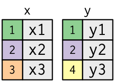
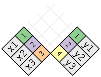
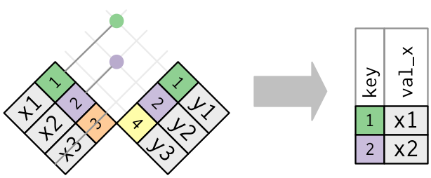
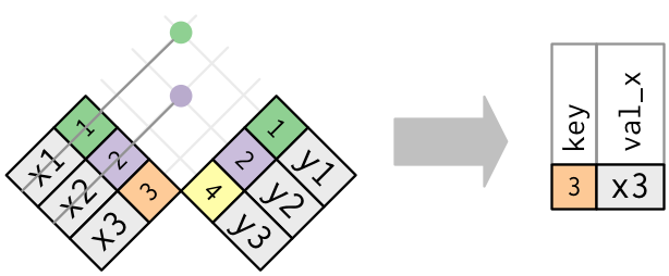
2.6.1 Left Join

The goal of a left join is to add variables from the data frame on the right (Y) to the data frame on the left (X) without duplicating any columns or adjusting the number of rows.

• What makes joins special is the data in the two data frames does not have to be sorted the same.
• A join operates on the basis of “key” fields which allow for matching a Key field in the X data frame to a corresponding “foreign” key field in the Y data frame.

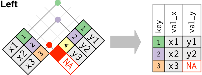
A left join looks like Figure 2.2 where the key fields 1 and 2 match so the values from the right data frame for those fields are added and the value for key field 3 gets an NA.

• Note, no rows are added or removed from the Left data frame.

Figure 2.2: Left Join of Data Frames X (left) and Y (right)

Let’s add variables from education (right) to the households data frame (left).

left_join(households, education) |> 
  glimpse()

Rows: 61
Columns: 10
$ Municipality            <chr> "Berat", "Kuçovë", "Poliçan", "Skrapar", "Dima…
$ Average_size            <dbl> 3.8, 3.8, 3.7, 3.7, 4.2, 4.6, 4.9, 3.7, 3.1, 3…
$ has_washing_machine     <dbl> 96.3, 95.5, 95.5, 94.5, 94.5, 92.6, 95.7, 87.7…
$ has_internet            <dbl> 71.4, 74.4, 52.8, 27.7, 80.0, 81.3, 85.1, 65.0…
$ has_computer            <dbl> 21.4, 14.8, 10.5, 12.3, 11.7, 14.0, 17.4, 10.6…
$ has_car                 <dbl> 36.9, 37.4, 26.3, 25.9, 46.2, 36.5, 39.2, 33.2…
$ Illiteracy_rate         <dbl> 2.7, 2.9, 4.8, 2.4, 2.5, 2.0, 2.7, 5.2, 3.0, 1…
$ primary_lower_secondary <dbl> 52.1, 49.1, 56.5, 52.8, 55.4, 56.4, 56.8, 59.7…
$ upper_secondary         <dbl> 33.9, 36.2, 31.9, 33.4, 31.4, 31.1, 29.1, 28.7…
$ university              <dbl> 13.2, 13.9, 10.8, 13.2, 12.1, 11.8, 13.6, 10.7…

• We get a message that the function found a common key field Municipality in both data frames and used that for the join.

Let’s try to add the variables from gdp_pop to our larger data frame.

left_join(households, education) |> 
  left_join(gdp_pop) |> 
  glimpse()

Error in `left_join()`:
! `by` must be supplied when `x` and `y` have no common variables.
ℹ Use `cross_join()` to perform a cross-join.

• Now we get an error because it cannot find common key fields.
• When we look at the data, we can see that gdp_pop has municipalities but they have the variable name gov_entity.
• We could rename the variable but that might mess up other places where we use that data.
• It is far better to use the join_by() function we saw in the first message.
  • join_by() allows us to specify how to connect the key fields in the two data frames.

left_join(households, education) |> 
  left_join(gdp_pop, join_by("Municipality" == "gov_entity")) |> 
  glimpse()

Rows: 61
Columns: 12
$ Municipality               <chr> "Berat", "Kuçovë", "Poliçan", "Skrapar", "D…
$ Average_size               <dbl> 3.8, 3.8, 3.7, 3.7, 4.2, 4.6, 4.9, 3.7, 3.1…
$ has_washing_machine        <dbl> 96.3, 95.5, 95.5, 94.5, 94.5, 92.6, 95.7, 8…
$ has_internet               <dbl> 71.4, 74.4, 52.8, 27.7, 80.0, 81.3, 85.1, 6…
$ has_computer               <dbl> 21.4, 14.8, 10.5, 12.3, 11.7, 14.0, 17.4, 1…
$ has_car                    <dbl> 36.9, 37.4, 26.3, 25.9, 46.2, 36.5, 39.2, 3…
$ Illiteracy_rate            <dbl> 2.7, 2.9, 4.8, 2.4, 2.5, 2.0, 2.7, 5.2, 3.0…
$ primary_lower_secondary    <dbl> 52.1, 49.1, 56.5, 52.8, 55.4, 56.4, 56.8, 5…
$ upper_secondary            <dbl> 33.9, 36.2, 31.9, 33.4, 31.4, 31.1, 29.1, 2…
$ university                 <dbl> 13.2, 13.9, 10.8, 13.2, 12.1, 11.8, 13.6, 1…
$ population                 <dbl> 62232, 31077, 8762, 10750, 28135, 26826, 50…
$ general_revenue_per_person <dbl> 16889, 17132, 98395, 32924, 14856, 21076, 1…

• Now this works fine.

Let’s save this to a new name and to our data folder.

left_join(households, education) |> 
  left_join(gdp_pop, join_by("Municipality" == "gov_entity")) ->
  house_ed_gdp_df

write_csv(house_ed_gdp_df, "./data/house_ed_gdp_joined.csv")

Having all this data in one place makes it easy to do some plots (more in the next chapters).

house_ed_gdp_df |> 
  ggplot(aes(x = Illiteracy_rate, y = general_revenue_per_person)) +
  geom_point() +
  labs(title = "Comparing Illiterarcy Rate and General Revenue Person for Municipalities",
       caption = "Data from Albania opendata.gv.al and INSTAT for 2023") +
  xlab("Illiteracy Rate") +
  ylab("General Revenue per Person") +
  scale_y_log10() + 
  geom_smooth(se = FALSE, linetype = 2, color = "red") +
  geom_smooth( method = "lm", se = FALSE)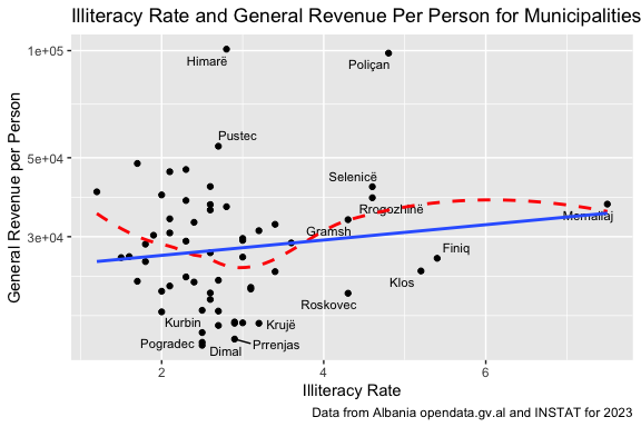

How would you interpret this graph? Do you believe it?

Note

There are other mutating joins such as the Full join, the right join and the inner join.

• A Right join is just a mirror version of the left join so you can usually do a left join.
• Both full joins and inner joins can lead to issues with your data so there is rarely a need for them in data science work.

2.6.2 Filtering Joins

The goals for a filtering join are not about adding variables to a data frame but about removing rows in the left (X) data frame based on the data in the right (Y) data frame.

• semi_join(): returns all rows from x with a match in y (deleting those without a match)
• anti_join(): returns all rows from x without a match in y (deleting those that do match)

The look like

(a) Semi Join between Data Frames X (left) and Y (right)

(b) Anti Join between Data Frames X (left) and Y (right)

Figure 2.3: Filtering joins between two data frames.

Say we want to find those municipalities that have a cultural site and look at their household data.

households |> semi_join(museums) |> 
  arrange(Municipality)

# A tibble: 12 × 6
   Municipality Average_size has_washing_machine has_internet has_computer
   <chr>               <dbl>               <dbl>        <dbl>        <dbl>
 1 Berat                 3.8                96.3         71.4         21.4
 2 Durrës                3.1                97.6         77.1         29.2
 3 Fier                  2.9                95.9         73.5         19.6
 4 Finiq                 2.7                94.6         32.1          7.8
 5 Gjirokastër           2.9                97.3         67.7         23.7
 6 Himarë                2.5                95.5         44.5         13.3
 7 Korçë                 2.8                96.4         80           33.4
 8 Krujë                 3.7                95           65.3         18.2
 9 Lezhë                 3.2                95.9         76.2         20.4
10 Sarandë               2.8                97.8         78.3         30.3
11 Shkodër               3.1                95.3         78.1         28.5
12 Vlorë                 2.7                97.4         67.8         23.8
# ℹ 1 more variable: has_car <dbl>

Only 12 Municipalities have cultural sites.

Does this make sense? There should be 13??

museums |> 
  select(Municipality) |> 
  distinct()

# A tibble: 13 × 1
   Municipality
   <chr>       
 1 Tirana      
 2 Durrës      
 3 Vlorë       
 4 Krujë       
 5 Berat       
 6 Korçë       
 7 Shkodër     
 8 Gjirokastër 
 9 Himarë      
10 Sarandë     
11 Finiq       
12 Fier        
13 Lezhë       

Now we want to find those that do Not have a cultural site

households |> anti_join(museums) |> 
    arrange(Municipality)

# A tibble: 49 × 6
   Municipality Average_size has_washing_machine has_internet has_computer
   <chr>               <dbl>               <dbl>        <dbl>        <dbl>
 1 Belsh                 3.8                94.1         84.6          9.5
 2 Bulqizë               4.6                92.6         81.3         14  
 3 Cërrik                3.9                93.9         80.5         11.2
 4 Delvinë               2.8                95           68.7         16.5
 5 Devoll                3.9                94.6         79.1         18.4
 6 Dibër                 4.9                95.7         85.1         17.4
 7 Dimal                 4.2                94.5         80           11.7
 8 Divjakë               3.1                95.7         82           13.6
 9 Dropull               2.8                97.4         29.7         13  
10 Elbasan               3.1                95.9         77.1         25.1
# ℹ 39 more rows
# ℹ 1 more variable: has_car <dbl>

What is going on??

museums |> 
  mutate(Municipality = str_replace(Municipality, "Tirana", "Tiranë")) ->
  museums
 
households |> 
 semi_join(museums) |> 
  arrange(Municipality)

# A tibble: 13 × 6
   Municipality Average_size has_washing_machine has_internet has_computer
   <chr>               <dbl>               <dbl>        <dbl>        <dbl>
 1 Berat                 3.8                96.3         71.4         21.4
 2 Durrës                3.1                97.6         77.1         29.2
 3 Fier                  2.9                95.9         73.5         19.6
 4 Finiq                 2.7                94.6         32.1          7.8
 5 Gjirokastër           2.9                97.3         67.7         23.7
 6 Himarë                2.5                95.5         44.5         13.3
 7 Korçë                 2.8                96.4         80           33.4
 8 Krujë                 3.7                95           65.3         18.2
 9 Lezhë                 3.2                95.9         76.2         20.4
10 Sarandë               2.8                97.8         78.3         30.3
11 Shkodër               3.1                95.3         78.1         28.5
12 Tiranë                2.9                98           80           49.3
13 Vlorë                 2.7                97.4         67.8         23.8
# ℹ 1 more variable: has_car <dbl>

Bottom line: Always check your data:)

2.7 Creating a New Variable

We saw earlier that we could create a new summary variable for population from the variables in the data frame and add it to the data frame.

Now let’s create a new variable for one data frame based on data in a second data frame.

• Let’s add a variable about whether a municipality has a cultural site and add it to the house_ed_gdp_df data frame.

• Let’s call the new variable culture_site and it will have two values: has_site and no_site.

  • This is a categorical variable (only a limited number of discrete possible values) so we will convert it to a factor.

• Look at the help for if_else() and as.factor().

house_ed_gdp_df |> 
  mutate(culture_site = if_else(
    Municipality %in% semi_join(households, museums)$Municipality, 
    "has_site", "no_site"
    ), .after = Municipality
  ) |> 
  mutate(culture_site = as.factor(culture_site))

# A tibble: 61 × 13
   Municipality culture_site Average_size has_washing_machine has_internet
   <chr>        <fct>               <dbl>               <dbl>        <dbl>
 1 Berat        has_site              3.8                96.3         71.4
 2 Kuçovë       no_site               3.8                95.5         74.4
 3 Poliçan      no_site               3.7                95.5         52.8
 4 Skrapar      no_site               3.7                94.5         27.7
 5 Dimal        no_site               4.2                94.5         80  
 6 Bulqizë      no_site               4.6                92.6         81.3
 7 Dibër        no_site               4.9                95.7         85.1
 8 Klos         no_site               3.7                87.7         65  
 9 Mat          no_site               3.1                90.9         67.5
10 Durrës       has_site              3.1                97.6         77.1
# ℹ 51 more rows
# ℹ 8 more variables: has_computer <dbl>, has_car <dbl>, Illiteracy_rate <dbl>,
#   primary_lower_secondary <dbl>, upper_secondary <dbl>, university <dbl>,
#   population <dbl>, general_revenue_per_person <dbl>

This appears to be working so let’s save to the data frame and rewrite to the data folder.

house_ed_gdp_df |> 
  mutate(culture_site = if_else(
    Municipality %in% semi_join(households, museums)$Municipality, 
    "has_site", "no_site"
    ), .after = Municipality
  ) |> 
  mutate(culture_site = as.factor(culture_site)) ->
  house_ed_gdp_df

write_csv(house_ed_gdp_df, "./data/house_ed_gdp_joined.csv")

• Note: when stored as a CSV file, it loses it’s class as a factor but that can be recreated upon reading it in.

You can check the levels of a factor with the levels() function.

levels(house_ed_gdp_df$culture_site)

[1] "has_site" "no_site" 

Factors are commonly used for trying to see if there is a difference between two or more categories.

house_ed_gdp_df |> 
  ggplot(aes(x = culture_site, y = population)) +
  geom_boxplot() +
 # scale_y_log10() +
  ggtitle("Municipalities with culture sites have a higher median population")

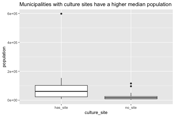
• Here we can see there is a clear difference in the median of the populations between municipalities that have a site and those that do not.

2.8 Summary

You have had a quick exposure to multiple tidyverse functions for manipulating data.

• There are more functions than we had time to cover.
• The goal was to give you some idea of the kinds of problems that can occur and the many ways data scientists can combine functions in creative strategies to solve a data cleaning and shaping problem.

Tip

A few keys to success:

1. Think about what you want your data to look like.
2. Use the Help function to understand how to use the function arguments to solve common problems.
3. Use the pipe to help build-a-little, test-a-little in a reproducible and clear way.
4. Forecast your results and check your data.
5. As always, save your work early and often:).

ASA, American Statistical Association. 1983. “Auto Data Set from the 1983 Exposition of Statistical Graphics Technology.” https://lib.stat.cmu.edu/data-expo/1983.html.

Barret, Tyson, Matt Dowle, Arun Srinivasan, Jan Goreck, Michael Chirico, Toby Hocking, Benjamin Schewndinger, and Ivan Krylob. 2025. “Data.table: Extension of ‘Data.frame‘.” https://r-datatable.com.

Bartley, Kevin. 2024. “Data Statistics (2025) - How Much Data Is There in the World?” Rivery. https://rivery.io/blog/big-data-statistics-how-much-data-is-there-in-the-world/.

Davenport, Thomas H., and D J. Patil. 2012. “Data Scientist: The Sexiest Job of the 21st Century.” Harvard Business Review October 2012: 70–76. http://hbr.org/2012/10/data-scientist-the-sexiest-job-of-the-21st-century/ar/1.

Firke, Sam. 2024. “Janitor: Simple Tools for Examining and Cleaning Dirty Data.” https://sfirke.github.io/janitor/.

Fox, John, and Sanford Weisberg. 2019. An {}R{} Companion to Applied Regression. Third. Sage. https://www.john-fox.ca/Companion/.

Friedman, Jerome, Trevor Hastie, and Robert Tibshirani. 2010. “Regularization Paths for Generalized Linear Models via Coordinate Descent{}.” Journal of Statistical Software 33 (1): 1–22. https://doi.org/10.18637/jss.v033.i01.

Godsey, Brian. 2017. Think Like a Data Scientist. Manning.

Grolemund, Garrett, and Hadley Wickham. 2011. “Lubridate: Dates and Times Made Easy with {Lubridate}.” Journal of Statistical Software 40 (3): 1–25. https://www.jstatsoft.org/v40/i03/.

———. n.d. R for Data Science. https://r4ds.had.co.nz/.

Horst, Allison, Alison Presmanes Hill, and Kristen B Gorman. 2020. “Palmerpenguins R Data Package.” https://doi.org/10.5281/zenodo.3960218.

Ian Fellows. 2022. “Wordcloud: Word Clouds.” Comprehensive R Archive Network. https://doi.org/10.32614/CRAN.package.wordcloud.

Institute of Statistics (INSTAT). 2025. “Statistical Database.” https://databaza.instat.gov.al:8083/pxweb/en/DST/.

Institute, QLB Brain. 2017. “Stunning Neuroscience Images.” https://qbi.uq.edu.au/blog/2017/07/stunning-neuroscience-images.

James, Gareth, Daniela Witten, Trevor Hastie, and Robert Tibshirani. 2023. An Introduction to Statistical Learning with Applications in R. 2nd ed. Springer. https://www.statlearning.com.

Kalinowski, Tomasz et al. 2022. “TensorFlow for R.” https://tensorflow.rstudio.com/.

Kalinowski, Tomasz, JJ Allaire, and François Chollet. 2025. “Keras3: R Interface to Keras.” https://keras3.posit.co/.

Kanwal, Maxinder S., Avinash S. Ramesh, and Lauren A. Huang. 2013. “A Novel Pseudoderivative-Based Mutation Operator for Real-Coded Adaptive Genetic Algorithms.” F1000Research. https://doi.org/10.12688/f1000research.2-139.v2.

Kaplan, Daniel, and Randall Pruim. 2023. “Ggformula: Formula Interface to the Grammar of Graphics.” https://www.mosaic-web.org/ggformula/.

Karatzoglou, Alexandros, Alex Smola, Kurt Hornik, National ICT Australia (NICTA), Michael A. Maniscalco, and Choon Hui Teo. 2024. “Kernlab: Kernel-Based Machine Learning Lab.” https://CRAN.R-project.org/package=kernlab.

Kelechava, Brad. 2018. “The SQL Standard - ISO/IEC 9075:2023 (ANSI X3.135).” The ANSI Blog. https://blog.ansi.org/sql-standard-iso-iec-9075-2023-ansi-x3-135/.

Khun, Max, and Julia Silge. 2023. Tidy Modeling with R. https://www.tmwr.org/.

Lin, Hause, and Tawab Safi. 2025. “Ollamar: An R Package for Running Large Language Models.” Journal of Open Source Software. https://doi.org/10.21105/joss.07211.

Myer, David. 2024. “E1071: Misc Functions of the Department of Statistics, Probability Theory Group.” https://cran.r-project.org/web/packages/e1071.

Neuroscientifically Challenged. 2014. “2-Minute Neuroscience: The Neuron.” https://www.youtube.com/watch?v=6qS83wD29PY.

Nohe, Patrick. 2017. “What Is the Dark Web?” https://www.thesslstore.com/blog/what-is-the-dark-web/.

“Ollama.” 2025. https://ollama.com.

“Open Data Inventory—Global Index of Open Data - Open Data Inventory.” n.d. Accessed May 8, 2025. https://odin.opendatawatch.com/.

Posit. 2025a. “Posit Cheatsheets.” https://posit.co/resources/cheatsheets/.

———. 2025b. “RStudio IDE User Guide.” RStudio User Guide. https://docs.posit.co/ide/user/.

“Quarto.” 2025. Posit.co. https://quarto.org/.

Rashida048. 2020. “Machine Learning: Gradient Descent Concept – Regenerative.” https://regenerativetoday.com/machine-learning-gradient-descent-concept/.

Robinson, Julia Silge and David. n.d. Text Mining with R. Accessed April 12, 2020. https://www.tidytextmining.com/.

Ruman. 2023. “Convex Vs. Non-Convex Functions: Why It Matters in Optimization for Machine Learning.” Medium. https://rumn.medium.com/convex-vs-non-convex-functions-why-it-matters-in-optimization-for-machine-learning-39cd9427dfcc.

Silge, Julia, and David Robinson. 2022. Tidytext: Text Mining with R. O’Reilly Media, Inc. https://www.tidytextmining.com/.

———. 2023. “Tidytext: Text Mining Using Tidy Tools.” https://juliasilge.github.io/tidytext/.

Sjoberg, Daniel D., Karissa Whiting, Michael Curry, Jessica A. Lavery, and Joseph Lamarange. 2021. “Reproducible Summary Tables with the Gtsummary Package.” The R Journal 13 (1): 570–80. https://doi.org/10.32614/RJ-2021-053.

Team, R Core. 2018. “R: A Language and Environment for Statistical Computing.” R Foundation for Statistical Computing. https://www.R-project.org/.

Ushey, Kevin, JJ Allaire, and Yuan Tang. 2023. “Reticulate: R Interface to Python.” https://rstudio.github.io/reticulate/.

van Rossum, Guido. 2025. “Python.” https://www.python.org/.

Waring, Elin, Michael Quinn, Amelia McNamara, Eduardo Arino d la RUbia, Shu Hao, and Shannon Ellis. 2025. “Skimr: Compact and Flexible Summaries of Data.” https://docs.ropensci.org/skimr/.

Wickham, Hadley. 2016. Ggplot2: Elegant Graphics for Data Analysis. Springer-Verlag New York. https://ggplot2.tidyverse.org/.

———. 2023a. “Forcats: Tools for Working with Categorical Variables (Factors).” https://forcats.tidyverse.org/.

———. 2023b. “Modelr: Modelling Functions That Work with the Pipe.” https://modelr.tidyverse.org/.

———. 2023c. “Stringr: Simple, Consistent Wrappers for Common String Operations.” https://stringr.tidyverse.org/.

Wickham, Hadley, Mara Averick, Jennifer Bryan, Winston Chang, Lucy D’Agostino McGowan, Romain Francois, Garret Grolemund, et al. 2019. “Welcome to the {Tidyverse}.” Journal of Open Source Software, no. 43: 1686. https://doi.org/10.21105/joss.01686.

Wickham, Hadley, Mine Cetinkaya-Rundel, and Garrett Grolemund. 2023. R for Data Science (2e). O’Reilly Media, Inc. https://r4ds.hadley.nz/.

Wickham, Hadley, Romain Francois, Lionel Henry, Kirill Muller, and Davis Vaughan. 2023. “Dplyr: A Grammar of Data Manipulation.” https://dplyr.tidyverse.org.

Wickham, Hadley, Jim Hester, and Jennifer Bryan. 2024. “Readr: Read Rectangular Text Data.” https://readr.tidyverse.org/.

Wickham, Hadley, Davis Vaughan, and Maximilian Girlich. 2023. “Tidyr: Tidy Messy Data.” https://tidyr.tidyverse.org.

Wikipedia. 2025. “Data Science.” Wikipedia. https://en.wikipedia.org/wiki/Data_science.