flowchart LR

A[R Script] --> B[HTTP Request]
B --> C[World Bank API]
C --> D[HTTP Response]
D --> E[JSON]
E --> F[R Objects]
12 Intro to Application Programming Interfaces (APIs)
Keywords
API, API Request, API Response, httr2, JSON, jsonlite
12.1 Introduction
In general purpose computing, application programming interfaces (APIs) allow one software system to request information or services from another software system.
- In data science, APIs are often used to retrieve current data from public data portals, government agencies, research databases, and commercial platforms.
- While many sites allow you to access and download data interactively, API’s allow you to get data programmatically which often allows you to get more specific with your requests and to get much more data faster.
This chapter uses APIs to introduce the same request-response pattern that is later used with large language model APIs.
- The immediate goal is to retrieve data from the World Bank Indicators API.
- The broader goal is to understand how a request is built, sent, checked, and parsed.
12.1.1 Learning Outcomes
By the end of this lesson, you should be able to:
- Explain what an API is and why APIs are useful in data science.
- Identify the main parts of an API request, including the base URL, endpoint, path parameters, and query parameters.
- Use
httr2to build and perform a basic HTTPGETrequest. - Use
jsonliteto parse a JSON response into R objects. - Convert API results into a tibble for analysis.
- Get data from the World Bank World Development Indicators API and conduct analysis.
12.1.2 References
- {httr2} R Package (Wickham 2023b)
- {jsonlite} R Package Ooms (2023)
- {tidyr} Rectangling Vignette Wickham, Vaughan, et al. (2023)
- {arrow} package (Neal Richardson et al. 2026)
- {keyring} R package Csardi (2022)
- World Bank Indicators API documentation (World Bank, n.d.-a)
- World Bank Indicator API queries (World Bank, n.d.-b)
- Eurostat API data access documentation (Eurostat, n.d.)
- Albania INSTAT API
12.1.2.1 Other References
12.2 APIs Allow Programmatic Access to Data
Organizations expose their data using an Application Programming Interface (API) when they want to allow others to access their data programmatically but they also want to use software to manage, monitor, and control the access to the data.
- APIs can perform multiple tasks; for data science, APIs are especially useful because they provide a repeatable way to get data.
- A script that uses an API can be tailored to get specific data and can often be used to get more data faster than by interacting with the web site.
APIs can control Who can access, What can be accessed, How can it be accessed, When it can be accessed, and What is returned.
- Who: An API may be “open” or require an API Key to access the data.
- The key may be free but required so they can monitor access.
- What: An API Endpoint is a location of a resource to be accessed by an API (think of an endpoint as aligned with a specific URL).
- APIs may act as gateways to many different endpoints which can be turned open or closed.
- How: APIs can provide access to data as a transaction as well as streaming data.
- The Representational state transfer or REST API is useful for accessing bulk data as a transaction.
- When: An API typically imposes limits on how much data can be transferred in a single request or across multiple requests during a specified time period.
- What is returned These days, most API will return data in one of two formats:
Organizations typically publish an API description document to provide users information on how to interact with the API across all these elements.
Note
APIs are an abstraction and can be implemented in many programming languages.
- We do not care how the API is coded; We only care about submitting our request for data in the proper format as specified by the API description document.
There are lots of free and public APIs: https://github.com/public-apis/public-apis. Table 12.1 shows just a few examples:
| API | Main topic | Description | API key? |
|---|---|---|---|
| World Bank Indicators API | Demographic, health, and economic indicators | Simple REST API for retrieving country-level time series | No |
| Eurostat Statistics API | European demographic, economic, regional, and social statistics | European statistical data using REST and JSON-stat | No |
| Open-Meteo API | Weather and climate data | Query parameters and geospatial requests | No |
| OpenAI API | Large language model responses and other AI services | Authenticated requests with JSON request bodies | Yes |
| Spotify Web API | Music, artists, albums, playlists, and audio features | OAuth authentication and nested JSON responses | Yes |
| GitHub REST API | Software repositories, users, and development activity | Authentication, pagination, and rate limiting | Optional |
| NASA Open APIs | Earth science, astronomy, imagery, and space missions | Public scientific APIs with JSON responses | Some endpoints |
| OpenStreetMap Nominatim API | Geocoding and geographic information | Location search and spatial data retrieval | No |
| Wikimedia REST API | Wikipedia content and metadata | Text retrieval and knowledge graph applications | No |
| The Movie Database (TMDb) API | Movies, actors, television, and ratings | Authentication and media metadata | Yes |
| Financial Modeling Prep API | Stock market and company financial data | Financial time series and economic analysis | Free key available |
| OECD Data API | International economic, education, labor, and social indicators | Multi-country statistical analysis | No |
| European Central Bank Data API | Inflation, exchange rates, and monetary policy indicators | European macroeconomic and financial analysis | No |
| World Health Organization API | Health, mortality, and disease indicators | Public health and epidemiological analysis | No |
| Census Bureau API | United States demographic and economic data | Structured query parameters and large datasets | Key recommended |
| INSTAT PX-Web API ALbania | Albania’s official statisticals | INSTAT (Instituti i Statistikave) statistical database | No |
This chapter uses the World Bank Indicators API because it is well documented, does not require an API key, and returns data in a format that can be parsed directly in R.
12.2.1 Interacting with an API
APIs can support a variety of HTTP methods for interacting with web sites as shown in Table 12.2.
| Method | Typical purpose | |
|---|---|---|
GET |
Retrieve data | |
POST |
Submit data or create a resource | |
PUT |
Replace or update a resource | |
PATCH |
Partially update a resource | |
DELETE |
Delete a resource |
We will generally only need GET although some APIs use POST per their documentation.
A simple workflow for getting data from a REST API has the following steps.
- Choose an endpoint (URL) that provides access to data of interest.
- Build a request by selecting arguments and values that adjust the endpoint URL to contain your request.
- Submit the request to the API. The API server then generates and returns a response.
- Check the response headers to see if your request was valid and the response body to check for the data you want.
- Parse the response body if it has the data you want.
- Save the data for future use.
TipAPI Keys and {keyring}
Many APIs require you to obtain an API key or personal access token (PAT) credential to establish your identity (you may have to register as a developer).
- Never put or display your private key/PAT in a file you might share such as a R script, .qmd, or .Rmd file.
A best practice is to store your API locally in your computer’s credential manager (as you did with your GitHub PAT).
- When working in R ,the {keyring} package allows you to use
keyring::key_set("my_key")to put your key into your computer’s credential manager (one time). - Then, every time you build an API request that requires a key, you can use
apikey = keyring::key_get(my_key)to automatically retrieve your key for the request.
This protects your key from appearing in the file and at the same time, it allows others to use the same code (as long as they use the same name for the key).
12.3 Using R for API Requests and Responses
We want to analyze the data on total population in Albania and eventually compare it to other countries and other data.
- While we could interact with the World Bank data site and download a file, we want to use an API so our work is documented in code, repeatable, and transparent.
Let’s write code to get data from the World Development Indicators API.
- This API provides access to tens of thousands of variables across over 250 countries.
We will follow the basic workflow in Figure 12.1.
12.3.1 R Packages
We will use two packages for working with APIs
- The
httr2package helps us send the request and receive the response. - The
jsonlitepackage helps us convert JSON text from the response body into R objects such as atomic vectors, data frames, and lists.
Use library() to load and attach the {tidyverse}, {httr2}, and {jsonlite} packages.
12.4 Build and Submit a Request with the {httr2} Package
The httr2 package helps with several tasks:
- Build a request object in steps
- Perform the request (send it to the API server)
- Receive the API response and check it.
Note
The {httr2} package uses several supporting packages, e.g., {curl}, which provides lower-level HTTP interfaces based on the curl library.
- You may see many references to using curl commands in the terminal in online discussions.
The World Bank Indicator API Queries identifies https://api.worldbank.org/v2/ as the initial URL from which you build endpoints by customizing the path.
- Let’s save that as the base URL.
Let’s use the request() function to create a request object we can use as a base for multiple requests.
<httr2_request>
GET https://api.worldbank.org/v2
Body: empty
Now that we have a base request object we want to modify it to get data on the total population for Albania over the last few decades.
- To do that we need to know the indicator code for total population and the country code for Albania.
- We can use our base request object to query the APIU and find out.
Let’s go quickly through the two examples of getting data for indicators and countries and then we will get into more detail for getting the population data for Albania.
12.4.1 Get An Indicator ID
There are over 29,000 indicator ID codes across all the World Bank databases (sources).
- The World Development Indicators (WDI) database contains many commonly used demographic, health, and economic measures which is what we want. It ID code Source = 2
The documentation shows we need to add values to the base URL path to tailor the endpoint and then add some fields to the query. Those are two different actions and each has its own function.
- Start with the base request and then pipe each step in sequence.
- Use
req_url_path_append()to add the terms"sources", "2", "indicators"to the URL path to make the endpoint, - Use
req_url_query()to add theper_pageargument with value 1500, (from API Basic Call Structures) and then, - Use
req_url_query()to add theformatargument after the path to tell it we want JSON output.- Note: When you look at the request object value, the
?in the `GET statement separates the endpoint path from the query fields.
- Note: When you look at the request object value, the
<httr2_request>
GET https://api.worldbank.org/v2/sources/2/indicators?per_page=1500&format=json
Body: empty
Now we can submit it and check our status from the response object.
[1] 200Let’s parse the response object to get some JSON data and convert to an R object.
Rows: 1,486
Columns: 7
$ id                 <chr> "AG.CON.FERT.PT.ZS", "AG.CON.FERT.ZS", "AG.LND.AGRI…
$ name               <chr> "Fertilizer consumption (% of fertilizer production…
$ unit               <chr> "", "", "", "", "", "", "", "", "", "", "", "", "",…
$ source             <df[,2]> <data.frame[26 x 2]>
$ sourceNote         <chr> "Fertilizer consumption measures the quantity of…
$ sourceOrganization <chr> "FAO electronic files and web site, Food and Agricu…
$ topics <list> [<data.frame[1 x 2]>], [<data.frame[1 x 2]>], [<dat…- We have a nice data frame with the 1,486 Indicators from the WDI we can use to identify and extract different variables from the API.
- How did I choose 1,500?
- The first time I ran the query the metadata in
indicator_json[[1]]$totalindicated that there were 1486 indicators in Source 2.
- The first time I ran the query the metadata in
- The API returned all 1,486 indicators because we requested
per_page = 1500. If the total exceeded the number returned per page, we would need to add an argument to retrieve additional pages. We’ll do that in the exercise.- Some APIs limit rows per page to 1,000 or less so you have to iterate over multiple pages.
How to find the actual code we want?
- We can use RStudio to manually filter the data frame.
- We can also use functions from the tidyverse {stringr} package to look for the words “Population” and “total” in the name field.
# A tibble: 11 × 2
   id                name
   <chr>             <chr>
 1 EN.POP.EL5M.ZS    Population living in areas where elevation is below 5 mete…
 2 EN.URB.MCTY.TL.ZS Population in urban agglomerations of more than 1 million …
 3 SP.POP.0014.TO    Population ages 0-14, total
 4 SP.POP.0014.TO.ZS Population ages 0-14 (% of total population)
 5 SP.POP.1564.TO    Population ages 15-64, total
 6 SP.POP.1564.TO.ZS Population ages 15-64 (% of total population)
 7 SP.POP.65UP.TO    Population ages 65 and above, total
 8 SP.POP.65UP.TO.ZS Population ages 65 and above (% of total population)
 9 SP.POP.TOTL       Population, total
10 SP.POP.TOTL.FE.ZS Population, female (% of total population)
11 SP.POP.TOTL.MA.ZS Population, male (% of total population) - Either way, we see
SP.POP.TOTLis the ID code we want.
12.4.2 Get the Country ID
Now we repeat the same steps: build the request object, perform the query, parse the response, and filter the data frame.
- Only this time, we just need to add “country” to the base request object path.
country_request <-
  request("https://api.worldbank.org/v2") |>
  req_url_path_append("country") |>
  req_url_query(
    format = "json",
    per_page = 500
  )

country_response <-
  country_request |>
  req_perform()

country_json <-
  country_response |>
  resp_body_json(simplifyVector = TRUE)

country_df <-
  country_json[[2]] |>
  as_tibble()

country_df|>
  filter(name =="Albania") |>
  select(id, name)
# A tibble: 1 × 2
id name
<chr> <chr>
1 ALB Albania- We can see the country ID code is “ALB”
12.4.3 Get the Total Population for Albania
We now know the ID codes for Country for Albania (“ALB”) and the indicator code for Total Population (SP.POP.TOTL).
- We start with the base request and then append country and indicator ID codes and add the format argument so we get JSON output.
Table 12.3 breaks down the elements of the URL request.
| URL component | Example | Meaning |
|---|---|---|
| Protocol | https |
The secure web protocol |
| Host | api.worldbank.org |
The server (endpoint) that provides the API |
| Version | v2 |
Version 2 of the API |
| Resource path | country/ALB/indicator/SP.POP.TOTL |
The country and indicator being requested |
| Query parameter | format=json |
Requests a JSON response |
Table 12.3 shows that a URL contains more structure than a simple website address. The endpoint and query parameters tell the API from where to get the data, what data to return and in what format.
- We could add additional arguments from API Basic Call Structures to adjust our query
We can submit the request as follows and save the response object.
Before we look at the response object, let’s explore the JSON format and the {jsonlite} package
12.4.3.1 The {jsonlite} Package
Most modern APIs can return data in JSON format. Before extracting data from an API response, we need to understand how JSON stores information.
JSON stores data using objects, arrays, and key-value pairs. A simple JSON object with four key:value pairs might look like this:
The jsonlite package helps us convert JSON text into R objects using fromJSON().
- This converts to a list since the values have different classes (two character and two integer)
$country
[1] "Albania"

$indicator
[1] "Population, total"

$year
[1] 2023

$value
[1] 2745972
Here is example of a JSON array where each element has the same key value pairs and the same number of each.
- It converts to a data frame.
          country year population
1         Albania 2023    2745972
2          Greece 2023   10341277
3 North Macedonia 2023    1826247
JSON can support many hierarchical data structures besides rectangular data.
- The following example has multiple nested observations so it is converted into a nested list.
- Top-level metadata (country)
- Nested metadata (indicator)
- Multiple observations (observations)
$country
[1] "Albania"

$indicator
$indicator$id
[1] "SP.POP.TOTL"

$indicator$name
[1] "Population, total"


$observations
  year   value
1 2023 2745972
2 2022 2761785
# A tibble: 2 × 2
year value
<int> <int>
1 2023 2745972
2 2022 2761785- The
$observationswere converted to a data frame element in the list so you can can quickly convert it to a tibble if you wish.
NoteNested Data and Complex Data
A benefit of APIs and JSON format is that it enables access to data that is not in rectangular format.
- Rectangular format is inefficient for data where variables may have different numbers of attributes.
- As an example, consider getting data about all the named actors in a set of award-winning movies.
- Some movies might have just two actors and others might have 15.
- This kind of data is often stored as a list instead of a data frame.
- These lists can be deeply nested, e.g., for each actor we also get the other award-winning movies in which they appeared.
The {tidyverse} includes the {tidyr} package which includes a number of functions for working with “messy” data, to include un-nesting the elements of interest in a deeply-nested list.
12.5 Check the Response Object
Before we can parse the data we need to check if our request was successfully processed.
12.5.0.1 Check the Status Code
The response object includes a status code which how the server responded to our request.
200 OKmeans our request processed correctly through the API. It does Not mean we got the data we want.204 No Contentmeans our request was accepted but did not return any content.400 Bad Requestmeans the API could not interpret our request.401 Unauthorizedmeans the apikey was not recognized or not validated.403 Forbiddenmeans the request is understood but not allowed404 Not Foundmeans the endpoint or resource was not found408 Time Outmeans it took too long to process due to a slow or broken internet connection.
200 is the desired result. Other codes are not always failures in your R code; they may indicate that the API URL, query parameters, or authentication details need to be corrected.
- Codes 204, 400, and 401 mean you should look at the query request and the help documentation for the API to ensure it is correct. Check for typos etc..
- Responses with status codes 4xx and 5xx are HTTP errors and {httr2} automatically turns these into R errors.
For a longer list consider status codes.
Our response object returned the following:
ImportantAPIS and Gateways
Many organizations put their APIs behind another layer of software called a Gateway.
- The Gateway handles authentication and managing the size and rate of requests.
- The API then focuses on how to get and return data for a valid request.
Unfortunately, Gateways documentation is not always accessible and they often use different parameters for managing the transaction than the API as they are managing overall system load, not just the API.
- If you get a negative response, e.g., invalid authentication or too many requests, that may be from the Gateway and not the API.
- If you can’t determine the issue, feel free to contact the support team for the API.
12.5.1 Check the Response Object Body Element
The response object is a named list and we can look at the names of the elements in a typical response.
[1] "method"      "url"         "status_code" "headers"     "body"
[6] "timing"      "request"     "cache"
Table 12.4 shows the type of content in each of these elements.
| Element | Description | Typical Use |
|---|---|---|
method |
The HTTP method used for the request, such as GET, POST, PUT, or DELETE. |
Verify how the API was accessed. |
url |
The complete URL sent to the server, including any query parameters. | Confirm the endpoint and request parameters. |
status_code |
Numeric code returned by the server indicating success or failure. Common values are 200 (success), 404 (not found), and 500 (server error). |
Check whether the request succeeded. |
headers |
Metadata about the response, such as content type, date, caching information, and server details. | Determine how the response should be processed. |
body |
The actual content returned by the API, often JSON, XML, HTML, or a file. | Extract and analyze the returned data. |
timing |
Information about how long different stages of the request took. | Measure API performance and diagnose slow requests. |
request |
The original httr2_request object used to create the response. |
Review the request configuration and parameters. |
cache |
Information about whether the response was retrieved from a cache rather than the server. | Improve efficiency and reduce repeated API calls. |
A typical workflow focuses on only three components:
[1] 200<httr2_headers>
date: Wed, 17 Jun 2026 17:32:51 GMT
content-type: application/json;charset=utf-8
server: cloudflare [1] 5b 7b 22 70 61 67 65 22 3a 31 2c 22 70 61 67 65 73 22 3a 32 2c 22 70 65 72- We have seen the
$status_codealready - We can access the
$headersfor troubleshooting at the HTTP level withresp_headers(). - The content we want is in the
$body. Note the RAW encoding with 2-character hexadecimal codes.
We can check if the body has any content with resp_has_body()
- This does not mean we have data, it could be an error message, we want to look at the contents.
- Although, the larger the body the more likely it has data.
We can use {httr2} functions to extract data from the body in formats other than RAW
- As a character string
- As JSON
- As HTML
- As XML
12.6 Convert, Tidy, and Clean the Response Body Content
We can convert the RAW content in the $body element to a single character value, albeit a pretty long one.
[1] 9838[1] "[{\"page\":1,\"pages\":2,\"per_page\":50,\"total\":66,\"sourceid\":\"2\",\"lastupdated\":\"2026-04-08\"},[{\"indicator\":{\"id\":\"SP.POP.TOTL\",\"value\":\"Population, total\"},\"country\":{\"id\":\"AL\",\"value\":\"Albania\"},\"countryiso3code\":\"ALB\",\"date\":\"2025\",\"value\":null,\"unit\":\"\",\"obs_status\":\"\",\"decimal\":0},{\"indicator\":{\"id\":\"SP.POP.TOTL\",\"value\":\"Population, total\"},\"country\":{\"id\":\"AL\",\"value\":\"Albania\"},\"countryiso3code\":\"ALB\",\"date\":\"2024\",\"value\":2377128,\"unit\":\"\",\"obs_status\":\"\",\"decimal\":0},{\"indicator\":{\"id\":\"SP.POP.TOTL\",\"value\":\"Population, total\"},\"country\":{\"id\":\"AL\",\"value\":\"Albania\"},\"countryiso3code\":\"AL"- This appears to have meta data at the start followed by population totals for Albania for each year in JSON format (note the “id” and “value” tags).
Let’s convert to JSON using fromJSON()
List of 2
 $ :List of 6
  ..$ page       : int 1
  ..$ pages      : int 2
  ..$ per_page   : int 50
  ..$ total      : int 66
  ..$ sourceid   : chr "2"
  ..$ lastupdated: chr "2026-04-08"
 $ :'data.frame':   50 obs. of  8 variables:
  ..$ indicator      :'data.frame': 50 obs. of  2 variables:
  .. ..$ id   : chr [1:50] "SP.POP.TOTL" "SP.POP.TOTL" "SP.POP.TOTL" "SP.POP.TOTL" ...
  .. ..$ value: chr [1:50] "Population, total" "Population, total" "Population, total" "Population, total" ...
  ..$ country        :'data.frame': 50 obs. of  2 variables:
  .. ..$ id   : chr [1:50] "AL" "AL" "AL" "AL" ...
  .. ..$ value: chr [1:50] "Albania" "Albania" "Albania" "Albania" ...
  ..$ countryiso3code: chr [1:50] "ALB" "ALB" "ALB" "ALB" ...
  ..$ date           : chr [1:50] "2025" "2024" "2023" "2022" ...
  ..$ value          : int [1:50] NA 2377128 2414095 2451636 2489762 2528480 2567801 2607733 2648285 2689469 ...
  ..$ unit           : chr [1:50] "" "" "" "" ...
  ..$ obs_status     : chr [1:50] "" "" "" "" ...
  ..$ decimal        : int [1:50] 0 0 0 0 0 0 0 0 0 0 ...
The output is a list with 2 elements
- The first element is a list of meta data.
- The second is a data frame with eight columns. -The
indicatorandcountrycolumns are packed data-frame columns. Each contains a small two-column data frame because the original JSON stored those values as nested objects.- This can happen when converting nested JSON data.
            id             value
1  SP.POP.TOTL Population, total
2  SP.POP.TOTL Population, total
3  SP.POP.TOTL Population, total
4  SP.POP.TOTL Population, total
5  SP.POP.TOTL Population, total
6  SP.POP.TOTL Population, total
7  SP.POP.TOTL Population, total
8  SP.POP.TOTL Population, total
9  SP.POP.TOTL Population, total
10 SP.POP.TOTL Population, total id value
1 AL Albania
2 AL Albania
3 AL Albania
4 AL Albania
5 AL Albania
6 AL Albania
7 AL Albania
8 AL Albania
9 AL Albania
10 AL AlbaniaLet’s use one of the handy {tidyr} functions to “unpack” the data frame.
# A tibble: 6 × 10
  indicator_id indicator_value   country_id country_value countryiso3code date
  <chr>        <chr>             <chr>      <chr>         <chr>           <chr>
1 SP.POP.TOTL  Population, total AL         Albania       ALB             2025
2 SP.POP.TOTL  Population, total AL         Albania       ALB             2024
3 SP.POP.TOTL  Population, total AL         Albania       ALB             2023
4 SP.POP.TOTL  Population, total AL         Albania       ALB             2022
5 SP.POP.TOTL  Population, total AL         Albania       ALB             2021
6 SP.POP.TOTL  Population, total AL         Albania       ALB             2020
# ℹ 4 more variables: value <int>, unit <chr>, obs_status <chr>, decimal <int>- Now we have a nice tibble we can continue to clean and analyze.
Converting to JSON is such a common task, {httr2} has a function to convert directly to JSON.
- Note: the default for the argument
simplyVectorisFALSEand we want it to be true.
If we look at the results we see they are the same as the two step process.
# A tibble: 6 × 10
  indicator_id indicator_value   country_id country_value countryiso3code date
  <chr>        <chr>             <chr>      <chr>         <chr>           <chr>
1 SP.POP.TOTL  Population, total AL         Albania       ALB             2025
2 SP.POP.TOTL  Population, total AL         Albania       ALB             2024
3 SP.POP.TOTL  Population, total AL         Albania       ALB             2023
4 SP.POP.TOTL  Population, total AL         Albania       ALB             2022
5 SP.POP.TOTL  Population, total AL         Albania       ALB             2021
6 SP.POP.TOTL  Population, total AL         Albania       ALB             2020
# ℹ 4 more variables: value <int>, unit <chr>, obs_status <chr>, decimal <int>- Let’s convert the `date from character to integer so it sorts properly.
# A tibble: 6 × 10
  indicator_id indicator_value   country_id country_value countryiso3code  date
  <chr>        <chr>             <chr>      <chr>         <chr>           <int>
1 SP.POP.TOTL  Population, total AL         Albania       ALB              2025
2 SP.POP.TOTL  Population, total AL         Albania       ALB              2024
3 SP.POP.TOTL  Population, total AL         Albania       ALB              2023
4 SP.POP.TOTL  Population, total AL         Albania       ALB              2022
5 SP.POP.TOTL  Population, total AL         Albania       ALB              2021
6 SP.POP.TOTL  Population, total AL         Albania       ALB              2020
# ℹ 4 more variables: value <int>, unit <chr>, obs_status <chr>, decimal <int>
12.7 Begin Analysis of the Data
Let’s do a quick plot to see what we have.
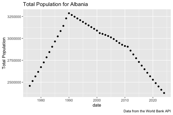
- The plot shows the population increased steadily through the 1970s and 1980s, peaked around 1990, and has been declining for more than three decades.
- We will explore these results by putting them into the context of other countries and other indicators in the exercise.
12.8 A Reusable Mental Model for Working with APIs
The API workflow can be summarized as follows:
The efficiency of the process depends upon several factors:
- A clear and comprehensive API description document that uses standard approaches so you can build valid request objects.
- A strategy for tidying and cleaning the data from the response object that isolates the data you need in a useful format. This requires a combination of Art and Science where the multiple functions and their arguments of {httr2}, {jsonLite}, and {tidyr} will be your friends.
Important
We will see this API workflow again when we work with Large Language Model APIs
12.9 Exercise 12: Build a Country Indicator Data set from an API
We want to use the World Bank Indicators API to retrieve demographic, health, and economic indicators for several countries using {httr2} and {{jsonlite}.
- In the previous sections, we focused on getting a single indicator for a single country.
- Now we will get data for multiple indicators for multiple countries and clean and tidy the data for analysis.
12.9.1 Setup
- Load packages {tidyverse}, {httr2}, {jsonlite}, {readxl}, and {arrow} packages (so we can work with files in parquet format).
- To build a feature rich data set we can identify a variety of categories that might affect population dynamics and a set of countries for comparison.
- We could filter the data frames we created earlier to find multiple indicators and their ID codes and countries and their ID codes.
- That would take some time so let’s start with a curated set of indicators and countries as shown in Table 12.5 and Table 12.6.
| Theme | Indicator | id_code | Why include it? |
|---|---|---|---|
| Demographics | Population, total | SP.POP.TOTL |
Main outcome for population change. |
| Demographics | Population growth, annual % | SP.POP.GROW |
Direct measure of population change rate. |
| Demographics | Fertility rate, total | SP.DYN.TFRT.IN |
Births per Woman. Long-run driver of population growth or decline. |
| Demographics | Birth rate, crude | SP.DYN.CBRT.IN |
Annual births per 1,000 people. |
| Demographics | Death rate, crude | SP.DYN.CDRT.IN |
Annual deaths per 1,000 people. |
| Demographics | Life expectancy at birth, total | SP.DYN.LE00.IN |
Broad health and demographic indicator. |
| Demographics | Urban population, % of total | SP.URB.TOTL.IN.ZS |
Indicates urbanization and structural change. |
| Labor market | Labor force participation rate, total | SL.TLF.CACT.ZS |
Share of working-age population active in the labor market. |
| Labor market | Employment to population ratio, 15+, total | SL.EMP.TOTL.SP.ZS |
Measures employment intensity relative to population. |
| Labor market | Unemployment, total | SL.UEM.TOTL.ZS |
Broad labor market stress indicator. |
| Labor market | Unemployment, youth total | SL.UEM.1524.ZS |
Youth labor market stress; often important for migration pressure. |
| Economy | GDP per capita, current US$ | NY.GDP.PCAP.CD |
Standard measure of average economic output per person. |
| Economy | GDP growth, annual % | NY.GDP.MKTP.KD.ZG |
Measures macroeconomic growth. |
| Economy | GNI per capita, Atlas method | NY.GNP.PCAP.CD |
Income-oriented alternative to GDP per capita. |
| Economy | Inflation, consumer prices | FP.CPI.TOTL.ZG |
Measures macroeconomic price instability. |
| Trade and investment | Exports of goods and services, % of GDP | NE.EXP.GNFS.ZS |
Measures export orientation and global integration. |
| Trade and investment | Imports of goods and services, % of GDP | NE.IMP.GNFS.ZS |
Measures import dependence and openness. |
| Trade and investment | Foreign direct investment, net inflows, % of GDP | BX.KLT.DINV.WD.GD.ZS |
Measures foreign investment relative to the economy. |
| Technology | Individuals using the Internet, % of population | IT.NET.USER.ZS |
Captures technology adoption and modernization. |
| Education | School enrollment, tertiary, gross % | SE.TER.ENRR |
Measures access to higher education. |
| Health | Infant mortality rate | SP.DYN.IMRT.IN |
Strong summary indicator of health and development. |
| Health | Current health expenditure, % of GDP | SH.XPD.CHEX.GD.ZS |
Measures national health spending effort. |
| Theme | Country | IC_code | Why include it? |
|---|---|---|---|
| Core case | Albania | ALB |
Main country of interest. |
| Neighbor | North Macedonia | MKD |
Nearby Balkan comparison with smaller population. |
| Neighbor | Greece | GRC |
Neighboring EU economy and migration destination. |
| Neighbor | Montenegro | MNE |
Nearby small Balkan country. |
| Neighbor | Serbia | SRB |
Larger western Balkan comparison. |
| Neighbor | Bosnia and Herzegovina | BIH |
Balkan comparison with post-socialist demographic change. |
| Regional comparison | Bulgaria | BGR |
EU Balkan comparison. |
| Regional comparison | Romania | ROU |
Larger regional EU comparison. |
| Regional comparison | Croatia | HRV |
EU comparison with population decline. |
| Regional comparison | Turkey | TUR |
Larger neighboring economy with different demographic pattern. |
Use read_exce() to read in the data from an excel file with two sheets called “indicators” and “countries” in the data folder.
- The file is called “world_bank_api_specs_balkans.xlsx”.
- Read each sheet into its own data frame: sheet “countries” to
country_tableand sheet “indicators” toindicator_table.
Glimpse each data frame.
- Note: the
read_excel()default istrim_ws = TRUEso undesirable white spaces at the beginning or end of the cell values are removed.
Rows: 10
Columns: 6
$ theme              <chr> "Core case", "Neighbor", "Neighbor", "Neighbor", "N…
$ country            <chr> "Albania", "North Macedonia", "Greece", "Montenegro…
$ id_code            <chr> "ALB", "MKD", "GRC", "MNE", "SRB", "BIH", "BGR", "R…
$ country_name       <chr> "Albania", "North Macedonia", "Greece", "Montenegro…
$ country_name_ascii <chr> "Albania", "North Macedonia", "Greece", "Montenegro…
$ why_include_it <chr> "Main country of interest for studying demographic …Rows: 22
Columns: 8
$ theme <chr> "Demographics", "Demographics", "Demographics", "De…
$ indicator <chr> "Population, total", "Population growth, annual %",…
$ source_id <dbl> 2, 2, 2, 2, 2, 2, 2, 2, 2, 2, 2, 2, 2, 2, 2, 2, 2, …
$ id_code <chr> "SP.POP.TOTL", "SP.POP.GROW", "SP.DYN.TFRT.IN", "SP…
$ variable_name <chr> "population_total", "population_growth", "fertility…
$ units <chr> "people", "percent", "births per woman", "births pe…
$ recommended_digits <dbl> 0, 1, 2, 1, 1, 1, 1, 1, 1, 1, 1, 0, 1, 0, 1, 1, 1, …
$ why_include_it <chr> "Main outcome for studying population size and long…
Tip
This workflow of reading in model specifications from an external file is common.
- It allows you to make changes to the specifications, e.g., add or delete a country or indicator, without changing the code file.
- It is a best practice to manage specifications or manually curated look-up tables as data files and not edit them inside the code.
- The API Basic Call Structures document includes an example for using Multiple Indicators:
Data for multiple indicators can be queried from a single data source by providing the indicator codes separated by “;” (semicolon), as well as the source ID.
We can do the same for both indicators and countries. Let’s create a character string for each with the appropriate codes and semicolons
- We can use
purrr::pull()to get the columns as a vector followed by andstringr::str_collapse()to convert to the semicolon-separated string for each.
Show code
[1] "ALB;MKD;GRC;MNE;SRB;BIH;BGR;ROU;HRV;TUR"[1] "SP.POP.TOTL;SP.POP.GROW;SP.DYN.TFRT.IN;SP.DYN.CBRT.IN;SP.DYN.CDRT.IN;SP.DYN.LE00.IN;SP.URB.TOTL.IN.ZS;SL.TLF.CACT.ZS;SL.EMP.TOTL.SP.ZS;SL.UEM.TOTL.ZS;SL.UEM.1524.ZS;NY.GDP.PCAP.CD;NY.GDP.MKTP.KD.ZG;NY.GNP.PCAP.CD;FP.CPI.TOTL.ZG;NE.EXP.GNFS.ZS;NE.IMP.GNFS.ZS;BX.KLT.DINV.WD.GD.ZS;IT.NET.USER.ZS;SE.TER.ENRR;SP.DYN.IMRT.IN;SH.XPD.CHEX.GD.ZS"12.9.2 Build a Request Object and Send it to the API
- The World Bank requires
;between the multiple codes but, unfortunately, thehttr2::req_url_query()function treats the;as reserved symbols and when it restructures the URL, it converts them to%which results in a bad request (status 404).
- You can get around this by building the entire URL manually using
stringr::str_glue(). - Start with 1000 observations per page.
https://api.worldbank.org/v2/country/ALB;MKD;GRC;MNE;SRB;BIH;BGR;ROU;HRV;TUR/indicator/SP.POP.TOTL;SP.POP.GROW;SP.DYN.TFRT.IN;SP.DYN.CBRT.IN;SP.DYN.CDRT.IN;SP.DYN.LE00.IN;SP.URB.TOTL.IN.ZS;SL.TLF.CACT.ZS;SL.EMP.TOTL.SP.ZS;SL.UEM.TOTL.ZS;SL.UEM.1524.ZS;NY.GDP.PCAP.CD;NY.GDP.MKTP.KD.ZG;NY.GNP.PCAP.CD;FP.CPI.TOTL.ZG;NE.EXP.GNFS.ZS;NE.IMP.GNFS.ZS;BX.KLT.DINV.WD.GD.ZS;IT.NET.USER.ZS;SE.TER.ENRR;SP.DYN.IMRT.IN;SH.XPD.CHEX.GD.ZS?source=2&format=json&per_page=1000- Create the request object with the complete URL.
<httr2_request>
GET https://api.worldbank.org/v2/country/ALB;MKD;GRC;MNE;SRB;BIH;BGR;ROU;HRV;TUR/indicator/SP.POP.TOTL;SP.POP.GROW;SP.DYN.TFRT.IN;SP.DYN.CBRT.IN;SP.DYN.CDRT.IN;SP.DYN.LE00.IN;SP.URB.TOTL.IN.ZS;SL.TLF.CACT.ZS;SL.EMP.TOTL.SP.ZS;SL.UEM.TOTL.ZS;SL.UEM.1524.ZS;NY.GDP.PCAP.CD;NY.GDP.MKTP.KD.ZG;NY.GNP.PCAP.CD;FP.CPI.TOTL.ZG;NE.EXP.GNFS.ZS;NE.IMP.GNFS.ZS;BX.KLT.DINV.WD.GD.ZS;IT.NET.USER.ZS;SE.TER.ENRR;SP.DYN.IMRT.IN;SH.XPD.CHEX.GD.ZS?source=2&format=json&per_page=1000
Body: empty- Submit the request and save the response.
12.9.3 Check and Parse the Response
- Check the status code.
- Parse the
response$bodyfrom JSON to R
List of 2
 $ :List of 6
  ..$ page       : int 1
  ..$ pages      : int 15
  ..$ per_page   : int 1000
  ..$ total      : int 14520
  ..$ sourceid   : NULL
  ..$ lastupdated: chr "2026-04-08"
 $ :'data.frame':   1000 obs. of  9 variables:
  ..$ indicator      :'data.frame': 1000 obs. of  2 variables:
  .. ..$ id   : chr [1:1000] "SP.POP.TOTL" "SP.POP.TOTL" "SP.POP.TOTL" "SP.POP.TOTL" ...
  .. ..$ value: chr [1:1000] "Population, total" "Population, total" "Population, total" "Population, total" ...
  ..$ country        :'data.frame': 1000 obs. of  2 variables:
  .. ..$ id   : chr [1:1000] "AL" "AL" "AL" "AL" ...
  .. ..$ value: chr [1:1000] "Albania" "Albania" "Albania" "Albania" ...
  ..$ countryiso3code: chr [1:1000] "ALB" "ALB" "ALB" "ALB" ...
  ..$ date           : chr [1:1000] "2025" "2024" "2023" "2022" ...
  ..$ value          : num [1:1000] NA 2377128 2414095 2451636 2489762 ...
  ..$ scale          : chr [1:1000] "" NA NA NA ...
  ..$ unit           : chr [1:1000] "" "" "" "" ...
  ..$ obs_status     : chr [1:1000] "" "" "" "" ...
..$ decimal : int [1:1000] 0 0 0 0 0 0 0 0 0 0 ...- Check the metadata in the first element of the parsed response including
page,pages,per_page, andtotal.
$page
[1] 1

$pages
[1] 15

$per_page
[1] 1000

$total
[1] 14520

$sourceid
NULL

$lastupdated
[1] "2026-04-08"- This says we got 1000 rows per page but there are 14,520 available.
- Unpack the observations in the second element data frame and use
slice_sample()to look at a random sample of rows from the observations to check the data.
Show code
# A tibble: 10 × 11
   indicator_id indicator_value   country_id country_value countryiso3code date
   <chr>        <chr>             <chr>      <chr>         <chr>           <chr>
 1 SP.POP.TOTL  Population, total BG         Bulgaria      BGR             1966
 2 SP.POP.TOTL  Population, total BG         Bulgaria      BGR             1962
 3 SP.POP.TOTL  Population, total BA         Bosnia and H… BIH             1990
 4 SP.POP.GROW  Population growt… HR         Croatia       HRV             1987
 5 SP.POP.TOTL  Population, total TR         Turkiye       TUR             2005
 6 SP.POP.TOTL  Population, total BA         Bosnia and H… BIH             1982
 7 SP.POP.GROW  Population growt… HR         Croatia       HRV             1989
 8 SP.POP.GROW  Population growt… GR         Greece        GRC             1985
 9 SP.POP.TOTL  Population, total RS         Serbia        SRB             1970
10 SP.POP.GROW  Population growt… BA         Bosnia and H… BIH             2021
# ℹ 5 more variables: value <dbl>, scale <chr>, unit <chr>, obs_status <chr>,
# decimal <int>- The data looks reasonable.
12.9.4 Get Multiple Pages
Since there are 15 pages worth of data, we can use {purrr} to iterate and get the data for each page.
- We will need to create two custom functions to generate the URL for a page and then to iterate for each page.
TipA Common Pattern in Data Science
We often need to perform the same operation many times.
- Retrieve multiple pages from an API.
- Analyze multiple files.
- Process multiple countries.
- Submit multiple prompts to an LLM.
The {purrr} package provides the map() family of functions for applying the same operation repeatedly and collecting the results.
- Provide a list or atomic vector of values and a function and it will apply the function to each element of the list and return the result.
- For those familiar with for-loops, map creates the for-loops for us, behind the scenes.
- We know there are 15 pages so use
seq_len()to create a sequence from 1 to 15
- Create a custom function with an argument for page to create the desired URL given the page argument.
- Use 1 as the default value for page.
https://api.worldbank.org/v2/country/ALB;MKD;GRC;MNE;SRB;BIH;BGR;ROU;HRV;TUR/indicator/SP.POP.TOTL;SP.POP.GROW;SP.DYN.TFRT.IN;SP.DYN.CBRT.IN;SP.DYN.CDRT.IN;SP.DYN.LE00.IN;SP.URB.TOTL.IN.ZS;SL.TLF.CACT.ZS;SL.EMP.TOTL.SP.ZS;SL.UEM.TOTL.ZS;SL.UEM.1524.ZS;NY.GDP.PCAP.CD;NY.GDP.MKTP.KD.ZG;NY.GNP.PCAP.CD;FP.CPI.TOTL.ZG;NE.EXP.GNFS.ZS;NE.IMP.GNFS.ZS;BX.KLT.DINV.WD.GD.ZS;IT.NET.USER.ZS;SE.TER.ENRR;SP.DYN.IMRT.IN;SH.XPD.CHEX.GD.ZS?source=2&format=json&per_page=1000&page=2- Create a custom function with an argument for page to retrieve and parse the data from the one page.
- Use the custom function just created to make the URL for the page.
- Use
mapto iterate across the sequence and get the data for each pagemap()returns a list of tibbles so we can uselist_rbind()to stack them one after the other into a single tibble.
Rows: 14,520
Columns: 11
$ indicator_id    <chr> "SP.POP.TOTL", "SP.POP.TOTL", "SP.POP.TOTL", "SP.POP.T…
$ indicator_value <chr> "Population, total", "Population, total", "Population,…
$ country_id      <chr> "AL", "AL", "AL", "AL", "AL", "AL", "AL", "AL", "AL", …
$ country_value   <chr> "Albania", "Albania", "Albania", "Albania", "Albania",…
$ countryiso3code <chr> "ALB", "ALB", "ALB", "ALB", "ALB", "ALB", "ALB", "ALB"…
$ date            <chr> "2025", "2024", "2023", "2022", "2021", "2020", "2019"…
$ value           <dbl> NA, 2377128, 2414095, 2451636, 2489762, 2528480, 25678…
$ scale           <chr> "", NA, NA, NA, NA, NA, NA, NA, NA, NA, NA, NA, NA, NA…
$ unit            <chr> "", "", "", "", "", "", "", "", "", "", "", "", "", ""…
$ obs_status      <chr> "", "", "", "", "", "", "", "", "", "", "", "", "", ""…
$ decimal <int> 0, 0, 0, 0, 0, 0, 0, 0, 0, 0, 0, 0, 0, 0, 0, 0, 0, 0, …- We have our raw data of 14,520 observations.
12.9.5 Clean the data
- The columns
unit,obs_status, anddecimalare metadata supplied by the World Bank API.
- They may be useful for publication formats but we don’t need them so let’s remove them.
- Let’s convert date to an integer
- Let’s rename some variables and reorder them as well
- Save with a new name
world_bank_raw_df |>
  select(-scale, -unit, -obs_status, - decimal) |>
  mutate(year = as.integer(date)) |>
    rename(
    indicator_code = indicator_id,
    indicator = indicator_value,
    country = country_value,
    country_code_2 = country_id,
    country_code_3 = countryiso3code,
  ) |>
  select(country, country_code_2, country_code_3, indicator,
         indicator_code, year, value) ->
  wb_clean

glimpse(wb_clean)
Rows: 14,520
Columns: 7
$ country <chr> "Albania", "Albania", "Albania", "Albania", "Albania", …
$ country_code_2 <chr> "AL", "AL", "AL", "AL", "AL", "AL", "AL", "AL", "AL", "…
$ country_code_3 <chr> "ALB", "ALB", "ALB", "ALB", "ALB", "ALB", "ALB", "ALB",…
$ indicator <chr> "Population, total", "Population, total", "Population, …
$ indicator_code <chr> "SP.POP.TOTL", "SP.POP.TOTL", "SP.POP.TOTL", "SP.POP.TO…
$ year <int> 2025, 2024, 2023, 2022, 2021, 2020, 2019, 2018, 2017, 2…
$ value <dbl> NA, 2377128, 2414095, 2451636, 2489762, 2528480, 256780…- We now have a set of clean data ready for analysis.
12.9.6 Save the Data
Because API calls depend on internet access and can be slow, we want to save the data after checking it.
Even though 14K records is not that large, let’s save as Parquet split by country_id.
Now that the data is saved, we do not have to re-run the api query, we can just load the data.
- We could create separate files for getting the data and for the analysis.
- This is especially useful when we are getting millions of records.
- As an alternative we could put the query perform and cleaning steps inside an “if-else” expression that checks if the data exists and loads it if true, else runs the query to get the data, clean it, and save it.
Rows: 14,520
Columns: 7
$ country        <chr> "Albania", "Albania", "Albania", "Albania", "Albania", …
$ country_code_2 <chr> "AL", "AL", "AL", "AL", "AL", "AL", "AL", "AL", "AL", "…
$ indicator      <chr> "Population, total", "Population, total", "Population, …
$ indicator_code <chr> "SP.POP.TOTL", "SP.POP.TOTL", "SP.POP.TOTL", "SP.POP.TO…
$ year           <int> 2025, 2024, 2023, 2022, 2021, 2020, 2019, 2018, 2017, 2…
$ value          <dbl> NA, 2377128, 2414095, 2451636, 2489762, 2528480, 256780…
$ country_code_3 <chr> "ALB", "ALB", "ALB", "ALB", "ALB", "ALB", "ALB", "ALB",…- Because the dataset is partitioned by
country_code_3, we could filter the collection and only load certain countries.
# A tibble: 1,452 × 7
   country country_code_2 indicator  indicator_code  year   value country_code_3
   <chr>   <chr>          <chr>      <chr>          <int>   <dbl> <chr>
 1 Albania AL             Populatio… SP.POP.TOTL     2025      NA ALB
 2 Albania AL             Populatio… SP.POP.TOTL     2024 2377128 ALB
 3 Albania AL             Populatio… SP.POP.TOTL     2023 2414095 ALB
 4 Albania AL             Populatio… SP.POP.TOTL     2022 2451636 ALB
 5 Albania AL             Populatio… SP.POP.TOTL     2021 2489762 ALB
 6 Albania AL             Populatio… SP.POP.TOTL     2020 2528480 ALB
 7 Albania AL             Populatio… SP.POP.TOTL     2019 2567801 ALB
 8 Albania AL             Populatio… SP.POP.TOTL     2018 2607733 ALB
 9 Albania AL             Populatio… SP.POP.TOTL     2017 2648285 ALB
10 Albania AL             Populatio… SP.POP.TOTL     2016 2689469 ALB
# ℹ 1,442 more rows
NoteTwo Country Code Systems
The World Bank API uses both two-character and three-character ISO country codes.
- In the original
countriesdata set theIDfield used the three character code, e.g., “ALB” and this is what was used in the request - However, the data that was returned from the WDI request uses the two character code for
country_idandcountryiso3codefor the three character code. - Both are valid but you need to be careful about which you are using, especially if making joins. (Always look at your data:))
12.9.7 Analyze the Data
- Look at a
summary()ofwb_cleanto check counts, unique values, and ranges
      country        country_code_2      indicator       indicator_code
 Length   :14520   Length   :14520   Length   :14520   Length   :14520
 N.unique :   10   N.unique :   10   N.unique :   22   N.unique :   22
 N.blank  :    0   N.blank  :    0   N.blank  :    0   N.blank  :    0
 Min.nchar:    6   Min.nchar:    2   Min.nchar:   17   Min.nchar:   11
 Max.nchar:   22   Max.nchar:    2   Max.nchar:   93   Max.nchar:   20


      year          value            country_code_3
 Min.   :1960   Min.   :     -28   Length   :14520
 1st Qu.:1976   1st Qu.:       6   N.unique :   10
 Median :1992   Median :      24   N.blank  :    0
 Mean   :1992   Mean   :  755035   Min.nchar:    3
 3rd Qu.:2009   3rd Qu.:      63   Max.nchar:    3
 Max.   :2025   Max.   :85518661
NAs :4443 - We have 22 unique indicators across 10 countries for years from 1960 to 2025 although there are 4,443 missing values.
- Population Trends
Figure 12.2 compares total population across the selected countries over time.
- Interpret the plot.
Show code
wb_clean |>
  filter(indicator_code == "SP.POP.TOTL") |>
  drop_na(year, value) ->
pop_df

pop_df |>
  group_by(country) |>
  filter(year == max(year)) |>
  ungroup() ->
pop_labels

pop_df |>
  ggplot(aes(x = year, y = value, color = country)) +
  geom_line(linewidth = 1) +
  ggrepel::geom_text_repel(
    data = pop_labels,
    aes(label = country),
    hjust = 0,
    nudge_x = 1,
    show.legend = FALSE
  ) +
  scale_y_log10(labels = scales::label_comma()) +
  scale_x_continuous(
    limits = c(min(pop_df$year), max(pop_df$year) + 8)
  ) +
  coord_cartesian(clip = "off") +
  labs(
    title = "Total Population by Country",
    subtitle = "Selected southeastern European countries",
    x = "Year",
    y = "Population (log scale)",
    color = "Country",
    caption = "Source: World Bank Indicators API"
  ) +
  theme(
    legend.position = "none",
    plot.margin = margin(5.5, 80, 5.5, 5.5)
  )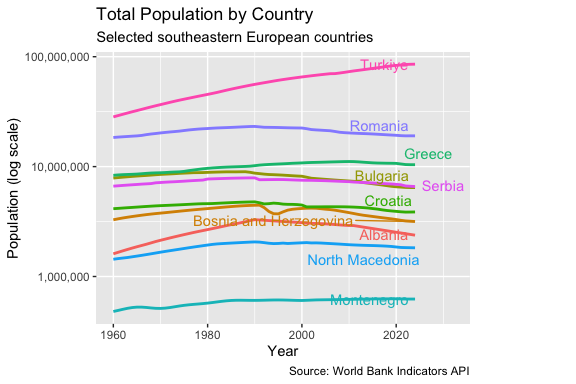
- Türkiye: strong sustained growth.
- Romania: growth followed by decline.
- Bulgaria, Croatia, Serbia, Albania: clear long-term population decline.
- Greece: growth followed by flattening and slight decline.
- Montenegro: essentially stable.
This begs the question: Can we figure out what might be happening using the other indicators?
NoteWhy Use a Log Scale?
The largest country in this dataset (Türkiye) has more than 100 times the population of the smallest country (Montenegro).
- A linear scale makes it difficult to see trends for the smaller countries because they are compressed near the bottom of the plot.
- A logarithmic scale spreads the countries apart and makes proportional changes easier to compare.
- Equal vertical distances correspond to similar percentage changes.
- The trade-off is that the actual population differences are less visually obvious.
- Reshape the data for multivariate analysis.
Let’s pivot the data wider to put each indicator into its own column so it is easier to do multi-variate analysis.
Rows: 660
Columns: 25
$ country                                                                                         <chr> …
$ country_code_3                                                                                  <chr> …
$ year                                                                                            <int> …
$ `Population, total`                                                                             <dbl> …
$ `Population growth (annual %)`                                                                  <dbl> …
$ `Fertility rate, total (births per woman)`                                                      <dbl> …
$ `Birth rate, crude (per 1,000 people)`                                                          <dbl> …
$ `Death rate, crude (per 1,000 people)`                                                          <dbl> …
$ `Life expectancy at birth, total (years)`                                                       <dbl> …
$ `Urban population (% of total population)`                                                      <dbl> …
$ `Labor force participation rate, total (% of total population ages 15+) (modeled ILO estimate)` <dbl> …
$ `Employment to population ratio, 15+, total (%) (modeled ILO estimate)`                         <dbl> …
$ `Unemployment, total (% of total labor force) (modeled ILO estimate)`                           <dbl> …
$ `Unemployment, youth total (% of total labor force ages 15-24) (modeled ILO estimate)`          <dbl> …
$ `GDP per capita (current US$)`                                                                  <dbl> …
$ `GDP growth (annual %)`                                                                         <dbl> …
$ `GNI per capita, Atlas method (current US$)`                                                    <dbl> …
$ `Inflation, consumer prices (annual %)`                                                         <dbl> …
$ `Exports of goods and services (% of GDP)`                                                      <dbl> …
$ `Imports of goods and services (% of GDP)`                                                      <dbl> …
$ `Foreign direct investment, net inflows (% of GDP)`                                             <dbl> …
$ `Individuals using the Internet (% of population)`                                              <dbl> …
$ `School enrollment, tertiary (% gross)`                                                         <dbl> …
$ `Mortality rate, infant (per 1,000 live births)`                                                <dbl> …
$ `Current health expenditure (% of GDP)` <dbl> …- We now have 660 rows of data. however some of the variable names are really long and almost all are non-syntactic, due to spaces or other characters, requiring the names to be delineated with `.
- We could have used the indicator code instead of the name. The codes are shorter but not human-readable unless you work with them a lot.
- Using the names means we will want to clean the names to be syntactically correct and then shorten many of them as well.
- These are common steps in this kind of data cleaning.
Let’s use janitor::clean_names() and then rename() to manually create shorter names we can still understand.
wb_wide |>
janitor::clean_names() |>
  rename(
    population_total = population_total,
    population_growth = population_growth_annual_percent,
    fertility_rate = fertility_rate_total_births_per_woman,
    birth_rate = birth_rate_crude_per_1_000_people,
    death_rate = death_rate_crude_per_1_000_people,
    life_expectancy_total = life_expectancy_at_birth_total_years,
    urban_population_percent = urban_population_percent_of_total_population,
    labor_force_participation_total = labor_force_participation_rate_total_percent_of_total_population_ages_15_modeled_ilo_estimate,
    employment_population_ratio = employment_to_population_ratio_15_total_percent_modeled_ilo_estimate,
    unemployment_total = unemployment_total_percent_of_total_labor_force_modeled_ilo_estimate,
    youth_unemployment = unemployment_youth_total_percent_of_total_labor_force_ages_15_24_modeled_ilo_estimate,
    gdp_per_capita_current_usd = gdp_per_capita_current_us,
    gdp_growth = gdp_growth_annual_percent,
    gni_per_capita_atlas_usd = gni_per_capita_atlas_method_current_us,
    inflation_consumer_prices = inflation_consumer_prices_annual_percent,
    exports_percent_gdp = exports_of_goods_and_services_percent_of_gdp,
    imports_percent_gdp = imports_of_goods_and_services_percent_of_gdp,
    fdi_net_inflows_percent_gdp = foreign_direct_investment_net_inflows_percent_of_gdp,
    internet_users_percent = individuals_using_the_internet_percent_of_population,
    school_enrollment_tertiary = school_enrollment_tertiary_percent_gross,
    infant_mortality_rate = mortality_rate_infant_per_1_000_live_births,
    health_expenditure_percent_gdp = current_health_expenditure_percent_of_gdp
  ) ->
  wb_wide
  glimpse(wb_wide)
Rows: 660
Columns: 25
$ country <chr> "Albania", "Albania", "Albania", "Alba…
$ country_code_3 <chr> "ALB", "ALB", "ALB", "ALB", "ALB", "AL…
$ year <int> 2024, 2023, 2022, 2021, 2020, 2019, 20…
$ population_total <dbl> 2377128, 2414095, 2451636, 2489762, 25…
$ population_growth <dbl> -1.5431439, -1.5431081, -1.5431567, -1…
$ fertility_rate <dbl> 1.341, 1.348, 1.355, 1.365, 1.371, 1.3…
$ birth_rate <dbl> 10.131, 10.244, 10.305, 10.512, 10.536…
$ death_rate <dbl> 8.457, 8.332, 8.709, 10.262, 9.080, 7.…
$ life_expectancy_total <dbl> 79.776, 79.602, 78.769, 76.844, 77.824…
$ urban_population_percent <dbl> 58.54636, 58.21061, 57.86435, 57.50772…
$ labor_force_participation_total <dbl> 64.006, 63.882, 62.161, 59.684, 59.367…
$ employment_population_ratio <dbl> 57.164, 57.066, 55.457, 52.836, 52.458…
$ unemployment_total <dbl> 10.689, 10.669, 10.785, 11.474, 11.639…
$ youth_unemployment <dbl> 25.582, 25.410, 24.543, 27.089, 26.422…
$ gdp_per_capita_current_usd <dbl> 11377.776, 9730.869, 7756.962, 7242.45…
$ gdp_growth <dbl> 4.0459285, 4.0154172, 4.8268006, 8.969…
$ gni_per_capita_atlas_usd <dbl> 9910, 8730, 7720, 6940, 5970, 5900, 54…
$ inflation_consumer_prices <dbl> 2.21587375, 4.75834555, 6.72520272, 2.…
$ exports_percent_gdp <dbl> 36.28487, 38.41882, 37.19708, 31.13306…
$ imports_percent_gdp <dbl> 43.16977, 43.93367, 47.50097, 44.45735…
$ fdi_net_inflows_percent_gdp <dbl> 6.323495, 6.900370, 7.579340, 6.757915…
$ internet_users_percent <dbl> 85.8638992, 83.1355916, 82.6136754, 79…
$ school_enrollment_tertiary <dbl> 84.14962, 64.72935, 62.64792, 59.96987…
$ infant_mortality_rate <dbl> 8.3, 8.3, 8.3, 8.3, 8.1, 8.0, 7.8, 7.7…
$ health_expenditure_percent_gdp <dbl> NA, 7.052403, 7.536462, 7.357504, 7.46…- Although the computer does not care, it might be better for humans to re-order the variables according to their general category.
Let’s use select() to reorder the variables so we can interpret our results more easily.
wb_wide |>
  select(
    country, country_code_3, year,

    # Demographics
    population_total, population_growth, fertility_rate, birth_rate,  death_rate,
    life_expectancy_total, infant_mortality_rate,  urban_population_percent,

    # Labor
    labor_force_participation_total, employment_population_ratio, unemployment_total,
    youth_unemployment,

    # Economy
    gdp_per_capita_current_usd, gni_per_capita_atlas_usd, gdp_growth, inflation_consumer_prices,

    # Trade
    exports_percent_gdp, imports_percent_gdp, fdi_net_inflows_percent_gdp,

    # Technology & Education
    internet_users_percent, school_enrollment_tertiary,

    # Health
    health_expenditure_percent_gdp
  ) ->
wb_wide- We are now ready to do some multivariate analysis.
- Let’s look at the pairwise correlations across the indicators.
- Interpret the plot
- Consider the relationship at the area level (demographics, economy, etc.) as well as individual variables.
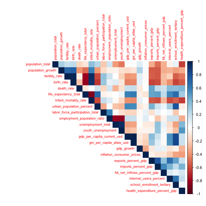
There is a lot to uncover in this plot given the multiple categories and variables within the categories.
Demographic Relationships
- Population growth is positively correlated with both fertility rate and birth rate.
- Fertility rate and birth rate are themselves highly correlated.
- Life expectancy and infant mortality exhibit one of the strongest relationships in the matrix.
- More urbanized countries tend to have lower fertility and population growth rates.
Labor Market Relationships
- Employment-to-population ratio is strongly negatively correlated with unemployment and youth unemployment.
- Unemployment and youth unemployment are highly positively correlated.
Economic Development Relationships
- GDP per capita, GNI per capita, Internet use, tertiary enrollment, and life expectancy form a clear development cluster in the bottom right
- These variables tend to move together across countries and over time.
- More economically developed countries generally exhibit higher incomes, greater Internet access, higher levels of educational attainment, and longer life expectancy.
Trade and Globalization Relationships
- Exports, imports, and foreign direct investment (FDI) are positively correlated.
- Countries that are more integrated into the global economy tend to: trade more, attract more foreign investment, and exhibit stronger connections to international markets.
Population Growth versus Development
- Population growth tends to be negatively correlated with GDP per capita,, internet use, tertiary enrollment, and life expectancy.
- This pattern is consistent with demographic transition theory; as countries become wealthier and more educated, fertility and population growth often decline.
Correlation Does Not Imply Causation
- This is observational data, not experimental data.
- These relationships do not necessarily imply direct causal effects.
- The correlations reflect both:
- Differences among countries, and
- Changes within countries over time.
- Additional analysis would be needed to identify causal mechanisms.
ImportantPreparing for LASSO Regression
The correlation matrix reveals several groups of variables that are highly correlated with one another.
- Fertility rate and birth rate
- GDP per capita and GNI per capita
- Unemployment and youth unemployment
- GDP per capita, Internet use, and tertiary enrollment
This phenomenon is known as multicollinearity.
- Multicollinearity can make it difficult for an ordinary regression model to determine which variable is most important because several predictors contain overlapping information.
LASSO regression addresses this problem by shrinking less important coefficients toward zero and often selecting a single representative variable from a highly correlated group.
- As a result, LASSO is a regularization method that can help identify which demographic, economic, labor-market, and development variables are most strongly associated with population growth while reducing the impact of redundant predictors.
The correlation plot serves as a useful bridge between exploratory data analysis and modeling.
12.9.8 Use a LASSO Regression Model to Explore Relationships
Let’s build a LASSO regression model to try to explore how the change in total population is associated with other indicators.
- We are more interested in how the population changes over time than in the total population so we’ll use
population_growthas our response instead of total population. - We have 20 remaining explanatory variables so LASSO can help identify which variables contribute most while reducing multicollinearity.
- Build the model data set by removing
country,country_code_3,population_totalandyearas not needed for the model.
- Why?
Note
Because the goal of this exercise is to explore relationships among variables rather than to build the most accurate predictive model, we fit the LASSO model using the full dataset.
- The
cv.glmnet()function uses cross-validation internally to select the tuning parameter \(\lambda\). - If the primary goal were prediction, we would typically reserve a separate test set that is not used during model fitting or model selection.
- Create the model matrix for the predictors and the vector for the response variable.
- Library {glmnet}, then build and run the model using use cross-validation to identify performance based on the size of the penalty.
- Save the results and plot the results.
- Interpret the plot.
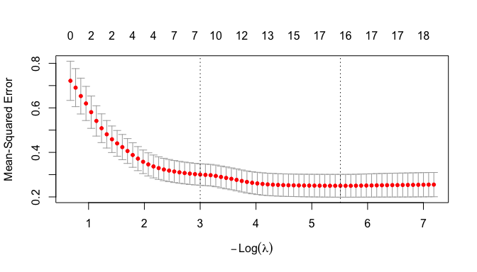
- Recall the following about the cross-validation curve.
- The numbers across the top are the number of variables with non-zero coefficients.
- The Y axis is the MSE performance metric obtained using cross-validation. The vertical bars show approximately \(\pm 1\) standard error across the folds.
- The X axis is based on the size of the penalty \(\lambda\); moving left means larger \(\lambda\) (stronger penalty: fewer variables) and moving right means smaller \(\lambda\) (weaker penalty: more variables).
- The left dotted line is the value for \(\lambda_{1SE}\) (the value to hedge against overfitting)
- The right dotted line is the value for \(\lambda_{min}\) which is the lowest MSE before overfitting inflates the MSE
- We can see this due to the cross-validation that holds out a different 1/10th of the data set for testing each of 10 models so no training data is used in evaluating the MSE.
Now let’s look at what we can see:
- Notice how flat the curve becomes.
- Error drops rapidly as we move from 0 predictors to roughly 9–12 predictors.
- After that, the gains in performance become very small.
- This tells us most of the predictive signal is captured by a relatively small subset of the variables.
- Adding additional predictors beyond that point produces only marginal improvements in performance.
- This suggests that many of the variables contain overlapping information.
- The correlation matrix hinted at this through several highly-correlated clusters of demographic, labor-market, and economic indicators.
- LASSO uses regularization to reduce the impact of this multicollinearity and identify a smaller set of predictors that capture most of the signal in population growth.
- Analyze the Coefficients
Let’s create a data frame of the coefficients for \(\lambda_{1SE}\) and \(\lambda_{min}\) and compare their values.
- Use a
left_join()to combine data frames of the variable coefficients into a single data frame. - Use
mutate()o add a new column of the difference between the coefficients - Arrange the rows by
lambda.1se, round the values and filter out the variables that are removed from both models.
Comment on the results
Show code
 left_join(
   (coef(lasso_cv, s = "lambda.1se") |>
  as.matrix() |>
  as.data.frame() |>
  rownames_to_column("variable")),
  (coef(lasso_cv, s = "lambda.min") |>
  as.matrix() |>
  as.data.frame() |>
  rownames_to_column("variable")),
  join_by(variable == variable) ) |>
  mutate(difference = lambda.1se - lambda.min) |>
  arrange(desc(abs(lambda.1se))) |>
  mutate(across(where(is.numeric), ~ round(.x, 3))) |>
  filter(lambda.1se !=0 | lambda.min !=0) ->
  lasso_compare
lasso_compare
variable lambda.1se lambda.min difference
1 (Intercept) -1.112 6.528 -7.640
2 fertility_rate 0.289 1.191 -0.902
3 birth_rate 0.127 0.001 0.127
4 labor_force_participation_total -0.046 -0.041 -0.005
5 death_rate -0.022 -0.095 0.073
6 urban_population_percent 0.019 0.034 -0.015
7 inflation_consumer_prices 0.004 0.010 -0.006
8 life_expectancy_total 0.000 -0.085 0.085
9 infant_mortality_rate 0.000 -0.043 0.043
10 employment_population_ratio 0.000 -0.015 0.015
11 gdp_growth 0.000 0.004 -0.004
12 exports_percent_gdp 0.000 -0.008 0.008
13 imports_percent_gdp 0.000 -0.002 0.002
14 fdi_net_inflows_percent_gdp 0.000 0.004 -0.004
15 internet_users_percent 0.000 0.002 -0.002
16 school_enrollment_tertiary 0.000 -0.010 0.010
17 health_expenditure_percent_gdp 0.000 -0.011 0.011The LASSO results indicate that fertility rate is the variable most strongly associated with population growth among the indicators considered.
- It has the largest coefficient in both models. Notice the dramatic drop after fertility rate.
- In the \(\lambda_{1SE}\) model, the coefficient for fertility rate is nearly five times larger than the coefficient for birth rate and roughly ten times larger than most of the remaining coefficients.
- These comparisons are meaningful because glmnet standardizes the predictor variables before fitting the model.
- Birth rate, mortality measures, labor-force participation, and urbanization also contribute to the model, but with substantially smaller coefficients.
- Economic development indicators such as GDP per capita, Internet use, and GNI per capita were removed by the more strongly regularized \(\lambda_{1SE}\) model.
- This does not imply that economic development is unrelated to population growth.
- Rather, it suggests that much of the association between economic development and population growth is already captured by demographic variables such as fertility, birth rates, and mortality.
- As the penalty is relaxed, additional variables are permitted to enter the model. The \(\lambda_{min}\) model therefore captures additional predictive signal beyond fertility, but the improvement is relatively small compared with the contribution of the demographic variables.
This result is consistent with demographic transition theory which argues that fertility and mortality are the primary drivers of long-run population growth, while economic development influences growth indirectly through its effects on those demographic factors.
Important
The \(\lambda_{1SE}\) and \(\lambda_{min}\) models are not nested ordinary regression models where additional variables are added while existing coefficients remain fixed.
- Instead, each value of \(\lambda\) produces a new LASSO optimization problem and a new set of coefficient estimates.
- As \(\lambda\) decreases, some variables enter the model, others may leave, and the coefficients of previously selected variables may increase or decrease as the model reallocates explanatory power among the predictors.
Because many predictors are highly correlated, the explanatory contribution of one variable depends on which other variables are currently included in the model.
- As \(\lambda\) changes and additional correlated predictors enter the model, the coefficients of existing variables may change substantially.
12.9.9 Back to Albania Data
- Let’s plot the variables with non-zero coefficients from the \(\lambda_{1se}\) model with population growth by their standardized values over time.
- note: Variables with negative LASSO coefficients (death rate and labor force participation) were multiplied by −1 before standardization so that all lines are oriented in the direction of increasing predicted population growth.
Show code
alb_df <-
  wb_wide |>
  filter(country == "Albania")

lasso_vars <- c(
  "population_growth",
  "fertility_rate",
  "birth_rate",
  "urban_population_percent",
  "death_rate",
  "labor_force_participation_total"
)

alb_df |>
  select(year, all_of(lasso_vars)) |>
  mutate(
    death_rate = -death_rate,
    labor_force_participation_total = -labor_force_participation_total
  )|>
  select(
    year,
    population_growth,
    fertility_rate,
    birth_rate,
    death_rate,
    labor_force_participation_total,
    urban_population_percent
  ) |>
  pivot_longer(
    -year,
    names_to = "variable",
    values_to = "value"
  ) |>
  group_by(variable) |>
  mutate(
    z = as.numeric(scale(value))
  ) |>
  ungroup() |>
  ggplot(
    aes(
      year,
      z,
      color = variable
    )
  ) +
  geom_line() +
  geom_point() +
  labs(
    y = "Standardized value (z-score)",
    x = NULL
  ) +
  labs(
  title = "Albania Population Growth and LASSO-Selected Indicators",
  subtitle = "Variables are standardized; \nNegatively signed predictors are reversed for visual comparison",
  x = "Year",
  y = "Standardized value (z-score)",
  color = "Variable",
  caption = "Source: World Bank Indicators API. \nDeath rate and labor force participation are multiplied by -1."
) +
  theme(
  legend.position = "top"
)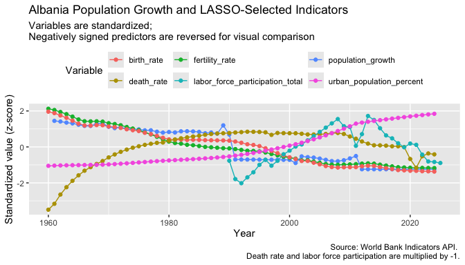
- The strongest visual relationship is between fertility rate and population growth.
- Both decline steadily over time, which supports the LASSO result that fertility rate is the variable most strongly associated with population growth.
- Birth rate follows a pattern very similar to fertility rate.
- This helps explain why the correlation matrix showed a strong relationship between the two variables and why LASSO assigned most of the explanatory power to fertility rate.
- Death rate, labor force participation, and urban population percentage exhibit trends that differ substantially from population growth.
- This demonstrates that variables can still contribute useful information in a multivariate model even when their time-series patterns do not closely resemble the response variable.
- The agreement between the time-series plot and the LASSO results provides additional evidence that demographic variables are more strongly associated with population growth than the economic variables included in this analysis.
NoteAn Important Lesson
The fertility rate provides an example where a variable that visually tracks population growth also receives a large LASSO coefficient.
- Note these were coefficients determined across all the countries in the model so reflect overall associations.
However, the other selected variables illustrate that visual similarity and statistical importance are not the same thing.
- A variable may have a weak visual relationship with the response variable yet still improve a multivariate model.
- Regression coefficients reflect relationships after accounting for the effects of the other variables in the model.
- This is one reason why multivariate modeling can reveal patterns that are not obvious from simple plots alone.
- Do the variables selected for population growth also appear related to total population?
- Let’s select the variables with the largest magnitude coefficients and plot against Total Population now.
- Facet on the indicator variable to allow for different X axes.
- Color by year as well.
Let’s get the four variables:
Show code
[1] "fertility_rate"                  "birth_rate"
[3] "labor_force_participation_total" "death_rate" - Now let’s plot and interpret the plot.
Show code
wb_wide |>
  filter(country == "Albania") |>
  select(
    year,
    population_total,
    all_of(top_lasso_vars)
  ) |>
  pivot_longer(
    cols = all_of(top_lasso_vars),
    names_to = "variable",
    values_to = "predictor_value"
  ) |>
  drop_na(population_total, predictor_value) |>
  ggplot(aes(x = predictor_value, y = population_total)) +
  geom_point(aes(color = year), alpha = 0.8) +
  geom_smooth (se = FALSE, color = "red", linewidth = .5) +
  facet_wrap(
    vars(variable),
    scales = "free_x"
  ) +
  scale_y_continuous(labels = scales::label_comma()) +
  labs(
    title = "Total Population and the Strongest LASSO-Selected Indicators",
    subtitle = "Albania only; predictors were selected by their association with population growth",
    x = "Predictor value",
    y = "Total population",
    color = "Year",
    caption = "Source: World Bank Indicators API"
  ) +
  theme(
  legend.position = "top"
)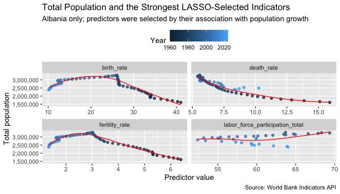
- The scatterplots reinforce the LASSO results by showing that fertility rate and birth rate have the strongest relationships with Albania’s long-run population trajectory.
- Death rate exhibits a weaker but still meaningful relationship, while labor force participation appears to contribute only modestly.
- Together, the visualizations and LASSO model suggest that demographic variables are more strongly associated with population change than the economic indicators included in this analysis.
12.9.10 Considering Albania in a Regional Context
The original plot showed a sharp decline in total population beginning in the early 1990s.
- This period coincided with major economic and social changes in Albania and was accompanied by declining fertility rates and increased migration.
- The LASSO model and subsequent visualizations suggest that demographic factors such as fertility and birth rates remain strongly associated with these long-run population trends.
At the same time, Albania’s long-run demographic patterns remain broadly consistent with those observed in neighboring countries.
- Fertility rates declined throughout southeastern Europe.
- Population growth slowed across the region.
- Urbanization increased.
- Educational attainment and internet use rose steadily.
As a result, Albania appears to have experienced an accelerated version of the broader demographic transition occurring across the Balkans rather than a completely unique demographic path.
12.10 Summary
This exercise demonstrated a complete workflow for working with a real-world API and transforming the returned data into a form suitable for analysis and visualization.
Key concepts included:
- Building API requests with {httr2}
- Creating reusable request objects.
- Modifying URL paths and query parameters.
- Submitting requests and inspecting response objects.
- Working with JSON data
- Converting JSON into R objects with {jsonlite}.
- Understanding the difference between lists, data frames, and nested (packed) data-frame columns.
- Using {tidyr} functions such as
unpack()to tidy nested structures.
- Discovering available data
- Querying the World Bank API to obtain lists of countries and indicators.
- Filtering these data frames to identify relevant country and indicator codes.
- Building requests dynamically from vectors of countries and indicators.
- Collecting and storing larger datasets
- Retrieving multiple pages of API results using iterative workflows with {purrr}.
- Combining results into a single tidy data frame.
- Saving the data in Parquet format for efficient reuse and reproducibility.
- Tidying and reshaping data
- Renaming variables to create meaningful and readable column names.
- Converting data from long to wide format using
pivot_wider(). - Preparing data for modeling and visualization.
- Exploratory data analysis
- Visualizing trends over time.
- Comparing countries and indicators.
- Using correlation matrices to identify relationships among variables.
- Recognizing potential multicollinearity among predictors.
- Regularized modeling with LASSO
- Using cross-validation to select an appropriate penalty parameter.
- Identifying the variables most strongly associated with population growth.
- Comparing the simpler \(\lambda_{1SE}\) model with the more complex \(\lambda_{min}\) model.
- Understanding how LASSO can select representative variables from highly correlated groups.
- Interpreting results in context
- Connecting statistical findings to demographic transition theory.
- Comparing Albania’s experience with broader regional trends.
- Using both visualization and modeling to support conclusions.
Most Important Takeaways
- APIs provide a repeatable way to collect large amounts of data directly from the source.
- JSON data often requires tidying before it can be analyzed effectively.
- Saving cleaned data locally improves efficiency and reproducibility.
- Visualization and exploratory analysis should precede modeling whenever possible.
- Correlation does not imply causation, but it can help identify useful relationships to investigate further.
- LASSO regression is a powerful tool for dealing with many correlated predictors and identifying the variables most strongly associated with an outcome.
- Domain knowledge remains essential; statistical models are most useful when interpreted within the context of the underlying subject matter.