Appendix A — A General Introduction to Matrices

A.1 Matrices, Vectors, and Scalars

A.1.1 Definition of a Matrix

A rectangular array is a set of numbers ( or symbols representing numbers) where the numbers are arranged in rows and columns where every column has the same number of rows and every row has the same number of columns.

A matrix is a rectangular array where each entry is called an element of the matrix. A matrix is often denoted by a capital letter, e.g., $A$.

A.1.2 The Size or Dimension of a Matrix

The size or dimension of a matrix $M$ is specified by the number of rows $r$ and the number of columns $c$ and is denoted as $(r\times c)$.

Alternative Notation: dim($M$) = $r\times c$

Examples:

Matrix $A$ has 3 rows and 2 columns so has size $(3\times 2)$ or dim($A$) = $3\times 2$.

$$A=\left[\begin{array}{cc}1& 2\\ 3& 0\\ -1& 4\end{array}\right]$$

Define matrix B

Matrix $B$ has 2 rows and 4 columns so has size $(2\times 4)$ or dim($B$) = $2\times 4$.

$$B=\left[\begin{array}{cccc}a& b& c& d\\ e& f& g& h\end{array}\right]$$

A.1.3 Row and Column Vectors

When a matrix only has one row it may be called a row vector with dimension $(1\times m)$. A vector $V$ may be denoted by $\overrightarrow{V}$.

• Think of the row vector as a row in a spreadsheet that contains all the values of the variables/attributes for one case or observation.

$$\overrightarrow{R}=\left[\begin{array}{cccc}0& -2& 0& 1\end{array}\right]$$

When a matrix only has one column, it may be called a column vector with dimensions $(n\times 1)$.

• Think of a column vector as a column in a spreadsheet with the values of the observations for one variable/attribute.

$$\overrightarrow{C}=\left[\begin{array}{r}10\\ -2\\ 0\\ 1\end{array}\right]$$

A.1.4 Scalars

A scalar is a matrix of size $(1\times 1)$ and is usually displayed as just the value as a real number.

ex. $k=\sqrt{2}$ is a scalar.

Warning

In the programming language R, a $(1\times 1)$ data frame is not the same as a single value. It is still of class data frame.

A.1.5 General Notation for a Matrix

If matrix $A$ has $n$ rows and $m$ columns, so dimension $(n\times m)$, each entry is called an element of $A$ and its position in the matrix is denoted using subscripts. The notation $a_{ij}$ identifies the element at the intersection of row $i$ and column $j$.

$$A=\left[\begin{array}{cccc}{a}_{11}& a_{12}& \cdots & a_{1m}\\ a_{21}& a_{22}& \cdots & a_{2m}\\ ⋮& ⋮& \ddots & ⋮\\ a_{n1}& a_{n2}& \cdots & a_{nm}\end{array}\right]$$

or, in shorthand, $A_{n\times m}$ is the set of $a_{ij}$ (where $\{\dots \}$ denotes a set), e.g., $$A=\left\{a_{ij}\right\}i=1,\dots ,n,j=1,\dots ,m$$

At times you may see the dimension of matrix indicated using a subscript so $A_{n\times m}$ means $A$ is a matrix with $n$ rows and $m$ columns.

A.2 Special Matrices

A.2.1 A Square Matrix

A square matrix is a matrix with the same number of columns and rows, i.e., of size $n\times n$. A square matrix of size $n\times n$ is said to be of order $n$.

$$Q=\left[\begin{array}{cc}1& 2\\ 3& 4\end{array}\right]$$

A.2.1.1 Determinants of Square Matrices

• Given a square matrix, one can calculate a scalar number known as the determinant of the matrix. The determinant of matrix $A$ is denoted in several ways: $det(A)=|A|$ or for a $2\times 2$ matrix as

$$det(A)=det\left[\begin{array}{cc}1& 3\\ 2& 4\end{array}\right]=\left|\begin{array}{cc}1& 3\\ 2& 4\end{array}\right|$$

• The determinant “determines” or describes how the matrix structure may affect other matrices when used in operations.

• The determinant of a matrix can be calculated using only the numbers in the matrix.

• For a matrix of order 2, the calculation is straightforward:

$$det(A)=\left|\begin{array}{cc}{a}_{11}& a_{12}\\ a_{21}& a_{22}\end{array}\right|=a_{11}{a}_{22}-a_{12}{a}_{21}$$

• For higher order matrices, the calculations get more complicated.

A.2.2 A Symmetric Matrix

A symmetric matrix $A$ is a square matrix where the elements that correspond by switching $i$ and $j$ are equal.

$$\left\{a_{ij}\right\}=\left\{a_{ji}\right\}\text{ for all }i=1,\dots ,n,j=1,\dots ,n$$

$$A=\left[\begin{array}{cccc}1& 2& 3& 4\\ 2& 5& 8& 9\\ 3& 8& 7& 10\\ 4& 9& 10& 11\end{array}\right]$$

A.2.3 A Diagonal Matrix

A diagonal matrix is a square matrix $(n\times n)$ where all the off diagonal elements are 0, i.e., the only non-zero elements are on the diagonal where $i=j$.

$$D=\left[\begin{array}{cccc}1& 0& 0& 0\\ 0& 3& 0& 0\\ 0& 0& -2& 0\\ 0& 0& 0& 10\end{array}\right]$$

Diagonal matrices are also symmetric.

A.2.4 The Identity Matrix

The Identity matrix is a diagonal matrix where every diagonal value is equal to 1 and all off-diagonal elements are 0.

$$I=\left[\begin{array}{cccc}1& 0& 0& 0\\ 0& 1& 0& 0\\ 0& 0& 1& 0\\ 0& 0& 0& 1\end{array}\right]$$

A.2.5 The $1_n$ and $0_n$ Vectors

A column vector of all 1s of size $(n\times 1)$ is denoted as

$$1_n=\left[\begin{array}{c}{1}_1\\ 1_2\\ ⋮\\ 1_n\end{array}\right]=\overrightarrow{1}$$

A column vector of all 0s of size $(n\times 1)$ is denoted as

$$0_n=\left[\begin{array}{c}{0}_1\\ 0_2\\ ⋮\\ 0_n\end{array}\right]=\overrightarrow{0}$$

A.3 Matrix Operations

A.3.1 Equality of Matrices

Definition: Two matrices $A$ and $B$ are said to be equal, denoted as $A=B$, if

$$\left\{a_{ij}\right\}=\left\{b_{ij}\right\}\text{ for all }i=1,\dots ,n,j=1,\dots ,m$$

Note

For two matrices to be equal they must be of the same size (dimension).

Example: If

$$A=\left[\begin{array}{cc}1& 2\\ 3& 0\\ -1& 4\end{array}\right]\text{ and }B=\left[\begin{array}{cc}x& 4/2x\\ \sqrt{9}& 2-2x\\ 3-4& 2^{2x}\end{array}\right]$$

then $A=B$ if $x=1$.

A.3.2 Addition of Matrices

To add two matrices $A,B$, they must have the same size, i.e., i.e., dim($A$)=dim($B$) = $n\times m$.

The addition of two matrices, $A+B$, results in the matrix $S$ where each element of $S$ is equal to the sum of the two corresponding elements of $A$ and $B$.

$$S=A+B\equiv \{s_{ij}=a_{ij}+b_{ij}\}\text{ for all }i=1,\dots ,n,j=1,\dots ,m$$

Example: if

$$A=\left[\begin{array}{cc}1& 2\\ 3& 0\\ -1& 4\end{array}\right]\text{ and }B=\left[\begin{array}{cc}-1& 4\\ 6& 0\\ 2& -3\end{array}\right]$$

then

$$A+B=\left[\begin{array}{cc}1+(-1)& 2+4\\ 3+6& 0+0\\ -1+2& 4+(-3)\end{array}\right]=\left[\begin{array}{cc}0& 6\\ 9& 0\\ 1& 1\end{array}\right]=S$$

A.3.3 Multiplying a Matrix by a Scalar

Let $k$ be any real number (a scalar) and $A$ a matrix of size $n\times m$.

Multiplying a matrix by a scalar results in a matrix where every element has been multiplied by the scalar.

$$kA=\left\{k{a}_{ij}\right\}\text{ for all }i=1,\dots ,n,j=1,\dots ,m$$

Example for matrix $A$,

$$\frac{1}{2}A=\frac{1}{2}\left[\begin{array}{cc}1& 2\\ 3& 0\\ -1& 4\end{array}\right]=\left[\begin{array}{cc}\frac{1}{2}(1)& \frac{1}{2}(2)\\ \frac{1}{2}(3)& \frac{1}{2}(0)\\ \frac{1}{2}(-1)& \frac{1}{2}(4)\end{array}\right]=\left[\begin{array}{cc}\frac{1}{2}& 1\\ \frac{3}{2}& 0\\ -\frac{1}{2}& 2\end{array}\right]$$

Note

Scalar multiplication is commutative: $kA=Ak$

A.3.4 Multiplying a Matrix by another Matrix

A.3.4.1 Definition

Let $A$ be an $n\times m$ matrix and $B$ be a $m\times k$ matrix.

Note

To multiply two matrices $A\text{ and }B$, the number of columns in $A$ must equal the number of rows in $B$, as seen here where $m=m$.

Multiplying $A$ $(n\times m)$ times $B$ $(m\times k)$, denoted as $AB$, results in a matrix $M$ of dimension $(n\times k)$ where $m_{ij}$ is the sum of the product of the corresponding elements in row $i$ from $A$ with the elements in the column $j$ from $B$ such that

$$AB=M\equiv \left\{m_{ij}\right\}\text{ for all }i=1,\dots ,n,j=1,\dots ,m$$

where

$$m_{ij}=(a_{i1}{b}_{1j}+a_{i2}{b}_{2j}+\cdots +a_{im}{b}_{mj})=\sum _{k=1}^m{a}_{ik}{b}_{kj}$$

Example:

$$\text{ Let }A=\left[\begin{array}{cc}1& 2\\ 3& 0\\ -1& 4\end{array}\right]\text{ and }B=\left[\begin{array}{cccc}2& 4& 6& 8\\ 1& 3& 5& 9\end{array}\right]$$

Here dim($A$) = $3\times 2$ and dim($B$) = $2\times 4$.

Therefore,

$$\begin{array}{rl}AB& =\left[\begin{array}{cccc}1(2)+2(1)& 1(4)+2(3)& 1(6)+2(5)& 1(8)+2(9)\\ 3(2)+0(1)& 3(4)+0(3)& 3(6)+0(5)& 3(8)+0(9)\\ -1(2)+4(1)& -1(4)+4(3)& 1(6)+4(5)& -1(8)+4(9)\end{array}\right]\\ & =\left[\begin{array}{cccc}4& 10& 16& 26\\ 6& 12& 18& 24\\ 2& 8& 14& 28\end{array}\right]\end{array}$$

A.3.4.2 Properties

1. Matrix multiplication is not commutative! If dim($B$) = $m\times k$ and dim($A$) = $n\times m$, the product $BA$ does not exist when $k\ne n$. If the $A$ and $B$ are both square with the same dimension then $BA$ may exist but it is not necessarily true that $BA=AB$.

2. Matrix multiplication is distributive under matrix addition such that for three matrices of the correct sizes, $A(B+C)=AB+AC$.

A.3.4.3 Exercises

A.3.4.3.1 Is matrix multiplication commutative?

$$\text{Let }C=\left[\begin{array}{cc}1& 4\\ 2& 3\end{array}\right]\text{ and }D=\left[\begin{array}{cc}4& 3\\ 5& 4\end{array}\right]$$

Compute $CD$ and $DC$ and check if $CD=DC$.

Solution

$$CD=\left[\begin{array}{cc}1(4)+4(5)& 1(3)+4(4)\\ 2(4)+3(5)& 2(3)+3(4)\end{array}\right]=\left[\begin{array}{cc}24& 19\\ 23& 18\end{array}\right]$$

and

$$DC=\left[\begin{array}{cc}4(1)+3(2)& 4(4)+3(3)\\ 5(1)+4(2)& 5(4)+4(3)\end{array}\right]=\left[\begin{array}{cc}10& 25\\ 13& 32\end{array}\right]$$

Warning

In matrix multiplication, order matters! Often $BA\ne AB$.

A.3.4.3.2 Is matrix multiplication distributive?

$$\text{Let }A=\left[\begin{array}{cc}1& 2\\ 3& 0\\ -1& 4\end{array}\right]B=\left[\begin{array}{cccc}2& 4& 6& 8\\ 1& 3& 5& 9\end{array}\right]\text{ and }C=\left[\begin{array}{cccc}1& 2& 3& 4\\ 5& 4& 3& 2\end{array}\right]$$

Check if $A(B+C)=AB+AC$

Solution

$$A(B+C)=\left[\begin{array}{cc}1& 2\\ 3& 0\\ -1& 4\end{array}\right]\left[\begin{array}{cccc}3& 6& 9& 12\\ 6& 7& 8& 11\end{array}\right]=\left[\begin{array}{cccc}15& 20& 25& 34\\ 9& 18& 27& 36\\ 21& 22& 23& 32\end{array}\right]$$

$$AB+AC=\left[\begin{array}{cccc}4& 10& 16& 26\\ 6& 12& 18& 24\\ 2& 8& 14& 28\end{array}\right]+\left[\begin{array}{cccc}11& 10& 9& 8\\ 3& 6& 9& 12\\ 19& 14& 9& 4\end{array}\right]=\left[\begin{array}{cccc}15& 20& 25& 34\\ 9& 18& 27& 36\\ 21& 22& 23& 32\end{array}\right]$$

A.3.4.4 Matrix Multiplication Terminology

$AB$ means we are pre-multiplying $B$ by $A$.

$BA$ means we are post-multiplying $B$ by $A$.

Depending upon the sizes of $A$ and $B$, neither $AB$ or $BA$ may exist or, if they exist, they may not be equal.

A.4 The Transpose of a Matrix

A.4.1 Definition

Let $A$ be an $n\times m$ matrix.

The transpose of $A$, denoted as $A^{⊺}$ or $A^{\prime }$, is the $m\times n$ matrix created by switching the columns of $A$ to become the rows of $A^{⊺}$. It can also be considered as rotating or flipping $A$ about its diagonal.

If $A=\left\{a_{ij}\right\}$ then $A^{⊺}=\left\{a_{ji}\right\}\text{ for all }i=1,\dots ,n,j=1,\dots ,m$

If

$$A=\left[\begin{array}{cccc}{a}_{11}& a_{12}& \cdots & a_{1m}\\ a_{21}& a_{22}& \cdots & a_{2m}\\ ⋮& ⋮& \ddots & ⋮\\ a_{n1}& a_{n2}& \cdots & a_{nm}\end{array}\right]$$

Then

$$A^{⊺}=\left[\begin{array}{cccc}{a}_{11}& a_{21}& \cdots & a_{n1}\\ a_{12}& a_{22}& \cdots & a_{2n}\\ ⋮& ⋮& \ddots & ⋮\\ a_{1m}& a_{2m}& \cdots & a_{mn}\end{array}\right]$$

Example:

$$\text{ If }A=\left[\begin{array}{cc}1& 2\\ 3& 0\\ -1& 4\end{array}\right]\text{ then }{A}^{⊺}=\left[\begin{array}{ccc}1& 3& -1\\ 2& 0& 4\end{array}\right]$$

Note

The transpose of a matrix always exists.

Tip

It is common in print to see column vectors represented as their transpose e.g., $$\overrightarrow{C}=\left[\begin{array}{c}1\\ 2\\ 3\end{array}\right]={\left[\begin{array}{ccc}1& 2& 3\end{array}\right]}^{⊺}$$

A.4.2 Properties of a Transpose

1. Identity:

$A^{⊺}=A$ if an only if $A$ is symmetric.

$$\text{ If }S=\left[\begin{array}{ccc}1& 2& 3\\ 2& 4& 6\\ 3& 6& 0\end{array}\right]\text{ then }{S}^{⊺}=\left[\begin{array}{ccc}1& 2& 3\\ 2& 4& 6\\ 3& 6& 0\end{array}\right]=S$$

2. Transpose under Multiplication

$(AB{)}^{⊺}=B^{⊺}{A}^{⊺}$

Warning

Notice when taking the transpose of a product, we switch the order when multiplying the product of the transposes.

Example:

$$\text{Let }A=\left[\begin{array}{cc}1& 2\\ 3& 4\end{array}\right]\text{ and }B=\left[\begin{array}{c}1\\ -1\end{array}\right]$$

so

$$A^{⊺}=\left[\begin{array}{cc}1& 3\\ 2& 4\end{array}\right]\text{ and }{B}^{⊺}=\left[\begin{array}{cc}1& -1\end{array}\right]$$

Then

$$AB=\left[\begin{array}{c}1(1)+2(-1)\\ 3(1)+4(-1)\end{array}\right]=\left[\begin{array}{c}-1\\ -1\end{array}\right]\text{ and }(AB{)}^{⊺}=\left[\begin{array}{cc}-1& -1\end{array}\right]$$

So

$$B^{⊺}{A}^{⊺}=\left[\begin{array}{c}1-1\end{array}\right]\left[\begin{array}{cc}1& 3\\ 2& 4\end{array}\right]=\left[\begin{array}{cc}1(1)+1(2)& 1(3)+-1(4)\end{array}\right]=\left[\begin{array}{cc}-1& -1\end{array}\right]$$

$$⟹(AB{)}^{⊺}=B^{⊺}{A}^{⊺}$$

Note

This property is often used, going both ways, in regression. You should be familiar with it.

A.5 More on the Determinant of A Square Matrix

1. If $A$ is any square matrix that contains a row (or column) or zeros, then $det(A)$ = 0.

Example: Let

$$F=\left[\begin{array}{cccc}1& 2& 3& 4\\ 0& 0& 0& 0\\ 2& 0& -2& 0\\ 1& 1& -5& 10\end{array}\right]$$

Then $det(F)$ = 0.

2. If $D$ is an $n\times n$ diagonal matrix, then $det(D)$ is the product of the entries on the main diagonal, i.e.,

$$det(D)=d_{11}{d}_{22}{d}_{33}...d_{nn}$$

Example: Let

$$D=\left[\begin{array}{cccc}1& 0& 0& 0\\ 0& 3& 0& 0\\ 0& 0& -2& 0\\ 0& 0& 0& 10\end{array}\right]$$ $$det(D)=1(3)(-2)(10)=-60.$$

3. If $A$ and $B$ are square matrices of the same size, then $det(AB)=det(A)det(B).$

A.6 The Inverse of a Matrix

A.6.1 Definition

A matrix $B$ is said to be the inverse of the matrix $A$ if

$$AB=I_n\text{ and }BA=I_n$$

If $B$ is the inverse of $A$ we denote the inverse as $B=A^{-1}$

A.6.2 Remarks

1. Only square matrices can have inverses.
2. Not All square matrices have inverses.
3. If $A^{-1}$ exists for matrix $A$, then the inverse $A^{-1}$ is unique.
4. If a matrix $A$ has an inverse, we say $A$ is invertible.
5. Matrix $A$ is invertible, if and only if $det(A)\ne 0$.

Proof:
If $A$ is an $n\times n$ invertible matrix, then there exists an $n\times n$ matrix $A^{-1}$ such that $A{A}^{-1}=I_n$,
where the identity matrix $I_n$ is a diagonal matrix with all 1’s on the diagonal.

$$det(A{A}^{-1})=det(A)det(A^{-1})=det(I_n)=1$$ Consequently $det(A)\ne 0$.

6. When $det(A)=0$ that means at least one row of the matrix can be calculated as a linear combination of other rows in the matrix. If $det(A)=0$, then we say the matrix $A$ is singular or non-invertible.
7. If $A$ is invertible, then the matrix equation $AX=B$ has a unique solution.

A.6.3 Calculating the Inverse of a Matrix

Calculating the inverse of a matrix of order 2 is straightforward:

$$\text{If }A=\left[\begin{array}{cc}a& b\\ c& d\end{array}\right]\text{ then }{A}^{-1}=\frac{1}{det(A)}\left[\begin{array}{cc}d& -b\\ -c& a\end{array}\right]=\frac{1}{ad-bc}\left[\begin{array}{cc}d& -b\\ -c& a\end{array}\right]$$

Note

Since the $det(A)$ appears in the denominator, when $det(A)=0$, $A^{-1}$ does not exist.

Warning

When calculating the determinant (or inverse) of a matrix using a computer, especially when the matrix is large or has values that differ by several orders of magnitude, special techniques are required to minimize the risk of getting values of 0 or close to 0 just due to the limited precision of a computer.

Example:

$$\text{Let }A=\left[\begin{array}{cc}1& 2\\ 3& 4\end{array}\right]\text{ then }det(A)=(1(4)-2(3))=-2$$

Define matrix $B$ as:

$$B=\frac{1}{-2}\left[\begin{array}{cc}4& -2\\ -3& 1\end{array}\right]=\left[\begin{array}{cc}-2& 1\\ 3/2& -1/2\end{array}\right]$$

Then

$$\begin{array}{rl}AB& =\left[\begin{array}{cc}1& 2\\ 3& 4\end{array}\right]\left[\begin{array}{cc}-2& 1\\ 3/2& -1/2\end{array}\right]=\left[\begin{array}{cc}1(-2)+2(3/2)& 1(1)+2(-1/2)\\ 3(-2)+4(3/2)& 3(1)+4(-1/2)\end{array}\right]\\ & =\left[\begin{array}{cc}1& 0\\ 0& 1\end{array}\right]=I_2\end{array}$$

and

$$\begin{array}{rl}BA& =\left[\begin{array}{cc}-2& 1\\ 3/2& -1/2\end{array}\right]\left[\begin{array}{cc}1& 2\\ 3& 4\end{array}\right]=\left[\begin{array}{cc}-2(1)+1(3)& -2(2)+1(4)\\ (3/2)(1)+(-1/2)(3)& (3/2)(2)+(-1/2)(4)\end{array}\right]\\ & =\left[\begin{array}{cc}1& 0\\ 0& 1\end{array}\right]=I_2\end{array}$$

$$⟹B=A^{-1}\text{ and }{A}^{-1}=B$$

A.6.4 Properties of the Inverse

Assuming an $A$, $B$ and $AB$ are invertible matrices, (i.e., $A^{-1}$, $B^{-1}$, and $(AB{)}^{-1}$ exist), then

1. $(A^{-1}{)}^{-1}=A$
2. $(AB{)}^{-1}=B^{-1}{A}^{-1}$

Warning

Notice when taking the inverse of a product, we switch the order when multiplying the product of the inverses.

A.6.4.1 Orthogonality

1. If $C$ is an $n\times n$ matrix, $C$ is said to be orthogonal if $C^{⊺}C=I_n$.
2. An $n\times n$ matrix $C$ is orthogonal if and only if $C^{-1}=C^{⊺}$.
3. The determinant of an orthogonal matrix is either 1 or -1.
4. Orthogonal matrices have nice properties such as enabling numerical stability in computer-based linear regression algorithms.

A.7 Linear Independence and the Rank of a Matrix

A.7.1 Definition of Linear Independence

Let ${\overrightarrow{V}}_1,{\overrightarrow{V}}_2,\dots ,{\overrightarrow{V}}_m$ be $m$ vectors and $k_1,k_2,\dots ,k_m$ be $m$ scalars.

The vectors ${\overrightarrow{V}}_1,{\overrightarrow{V}}_2,\dots ,{\overrightarrow{V}}_m$ are said to be linearly dependent if there exists some $k_i^{\prime }s\ne 0i=1,2\dots ,m$ such that the linear combination:

$$k_1{\overrightarrow{V}}_1+k_2{\overrightarrow{V}}_2+\cdots +k_m{\overrightarrow{V}}_m=\overrightarrow{0}=0_m$$

Note

If the vectors ${\overrightarrow{V}}_1,{\overrightarrow{V}}_2,\dots ,{\overrightarrow{V}}_m$ are linearly dependent, this implies there is at least one of the vectors ${\overrightarrow{V}}_i$ which can be expressed (calculated) as a linear combination of one or more of the other vectors.

Practical Interpretation: If a set of vectors is linearly dependent, then at least one of the vectors is redundant (does not add any new information to the other vectors).

Example:

$$\text{Let }S=\left[\begin{array}{ccc}1& 2& 3\\ 2& 4& 6\\ 3& 6& 0\end{array}\right]\text{ with row vectors }\begin{array}{cc}{\overrightarrow{V}}_1& =\left[\begin{array}{ccc}1& 2& 3\end{array}\right]\\ {\overrightarrow{V}}_2& =\left[\begin{array}{ccc}2& 4& 6\end{array}\right]\\ {\overrightarrow{V}}_3& =\left[\begin{array}{ccc}3& 6& 0\end{array}\right]\end{array}$$

$${\overrightarrow{V}}_2=2{\overrightarrow{V}}_1⟹(-2)\times {\overrightarrow{V}}_1+1\times {\overrightarrow{V}}_2+0\times {\overrightarrow{V}}_3=\overrightarrow{0}⟹\text{ the vectors are linear dependent}$$

If a set of vectors ${\overrightarrow{V}}_1,{\overrightarrow{V}}_2,\dots ,{\overrightarrow{V}}_m$ are not linearly dependent, they are said to be linearly independent.

Practical Interpretation: If a set of vectors is linearly independent, then all vectors contribute new information.

Note

Either row vectors or column vectors can be linearly dependent.

• Row vectors: Cases can be repeated so have identical information.
• Column vectors: Variables contain similar or redundant information.

A.7.2 Definition of the Rank of a Matrix

The rank of a matrix is the maximum number of linearly independent columns (rows).

A.7.3 Properties

1. The inverse of a $n\times n$ matrix $Q$ exists if an only if $rank(Q)=n$. We say $Q$ is of full rank.
2. For an $n\times m$ matrix $A$, $rank(A)\le min\{n,m\}$.
3. if $C=AB$, then $rank(C)\le min\{rank(A),rank(B)\}$.

A.8 Probability Results for Random Vectors

A.8.1 Definitions for a Random Vector.

Let $X_1,X_2,\dots ,X_k$ be a set of $k$ random variables.

A vector $X$ is a random vector when each element $X_i$ is a random variable, e.g.,

$$\overrightarrow{X}=\left[\begin{array}{c}{X}_1\\ X_2\\ ⋮\\ X_k\end{array}\right]\text{ is a random vector.}$$

Note

Since each random variable $X_i$ has a probability distribution, the random vector $X$ has what we refer to as a joint distribution.

The joint distribution describes how the $\{X_1,X_2,\dots ,X_k\}$ are distributed in relation to one another.

Given a random vector $\overrightarrow{X}$,

1. The expected value of $\overrightarrow{X}$ is the mean vector of $\overrightarrow{X}$ and represents the center of the joint distribution of $\overrightarrow{X}$. This is denoted as:

$${\overrightarrow{\mu }}_{\overrightarrow{X}}=E(\overrightarrow{X})=\left[\begin{array}{c}E(X_1)\\ E(X_2)\\ ⋮\\ E(X_k)\end{array}\right]$$

2. Given a $k$-dimensional random variable $X$, there exists a $k\times k$ symmetric matrix, $Cov(X)$, called the variance-covariance or covariance matrix of $X$. It has the form:

$$\begin{array}{}\text{(A.1)}& Cov(X)=\left[\begin{array}{cccc}Var(X_1)& Cov(X_1,X_2)& \cdots & Cov(X_1,X_k)\\ Cov(X_2,X_1)& Var(X_2)& \cdots & Cov(X_2,X_k)\\ ⋮& ⋮& ⋮& ⋮\\ Cov(X_k,X_1)& Cov(X_k,X_2)& \cdots & Var(X_k)\end{array}\right]\end{array}$$

Note

1. $Var(X_i)$ is equivalent to the variance of just the random variable $X_i$ itself.

2. $Cov(X_i,X_j)=E[(X_i-E[X_i])(X_j-E[X_j])=E[(X_i-{\mu }_i)(X_j-{\mu }_j)]$ provides us information on how the random variables $X_i,X_j$ are related (distributionally).

3. If $Cor(X_i,X_j)=\frac{Cov(X_i,X_j)}{\sqrt{Var(X_i)Var(X_j)}}=0$, then $X_i,X_j$ are uncorrelated.

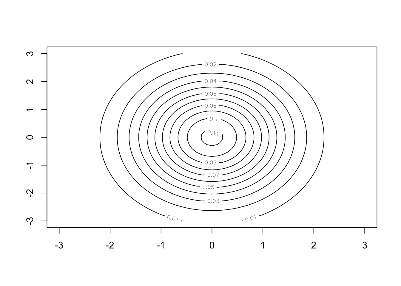
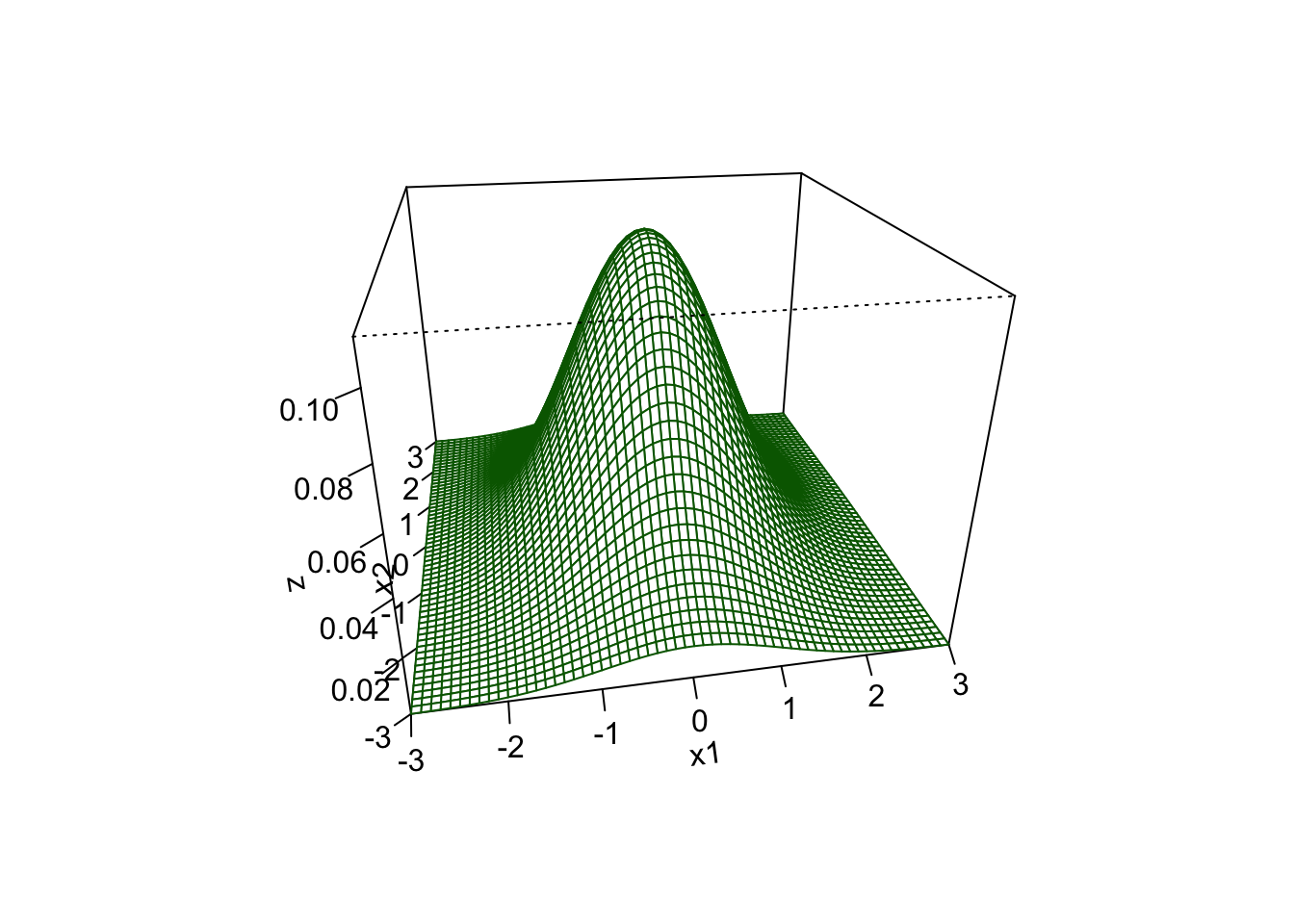
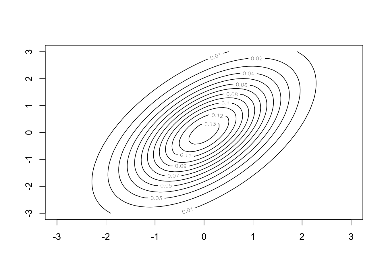
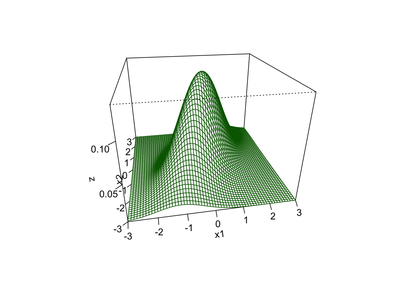
Example: Contour and surface plots of the joint density function of two normally distributed random variables with a joint distribution.

• In the first case, the two variables are independent, i.e., covariance is 0. The contour plot makes it easy to see $\text{Var}(X_2)>\text{ Var}(X_1)$.
• In the second case, the covariance is greater than zero. The contour plot shows how the values of $X_1$ and $X_2$ are related and that creates an angle in the joint density function.

(a) Cov = 0 Contour

(b) Cov = 0 Surface

(c) Cov = .8 Contour

(d) Cov = .8 Surface

Figure A.1: Bivariate Normals N(0,1), N(0,2)

A.8.2 Definition of a Multivariate Normal Distribution

A random vector $\overrightarrow{X}$ has a multivariate normal distribution if its probability density function (pdf) is given by:

$$\begin{array}{}\text{(A.2)}& f(\overrightarrow{X})=\frac{1}{(2\pi {)}^{k/2}|\mathrm{\Sigma }{|}^{1/2}}{e}^{-\frac{1}{2}(\overrightarrow{X}-\overrightarrow{\mu }{)}^{⊺}{\mathrm{\Sigma }}^{-1}(\overrightarrow{X}-\overrightarrow{\mu })}\end{array}$$

where: $\overrightarrow{\mu }=E[\overrightarrow{X}],\mathrm{\Sigma }=Cov(\overrightarrow{X}{)}_{k\times k}$ and $|\mathrm{\Sigma }|$ denotes the determinant of $det(\mathrm{\Sigma })$.

The joint Normal distribution of $\overrightarrow{X}$ is denoted by $\overrightarrow{X}\sim N_k(\overrightarrow{\mu },\mathrm{\Sigma })$.

A.8.3 Properties

1. If $\overrightarrow{X}\sim N_k(\overrightarrow{\mu },\mathrm{\Sigma })$, then the marginal distribution of $X_i$ is $\sim N({\mu }_i,{\sigma }_i^2)$.
2. If $Cor(x_i,x_j)=0\text{ for all }i\ne j$ then

$$\mathrm{\Sigma }=\left[\begin{array}{cccc}{\sigma }_1^2& 0& \cdots & 0\\ 0& {\sigma }_2^2& \cdots & 0\\ ⋮& ⋮& \cdots & ⋮\\ 0& 0& \cdots & {\sigma }_k^2\end{array}\right]$$

and $x_1,\dots ,x_k$ are independent normally-distributed random variables.

A.9 Matrices and the Classic Multiple Linear Regression Model

Let there be $p-1$ predictor/explanatory variables $X_1,\dots ,X_{p-1}$.

Assume the true model is:

$$\begin{array}{}\text{(A.3)}& Y_i={\beta }_0+{\beta }_1{X}_{i1}+{\beta }_2{X}_{i2}+\cdots +{\beta }_{p-1}{X}_{i,p-1}+{ϵ}_{i}i=1,\dots ,n\end{array}$$

The Equation A.3 model can also be written as a set of $n$ equations:

$$\begin{array}{rl}{Y}_1& ={\beta }_0+{\beta }_1{X}_{11}+{\beta }_2{X}_{12}+\cdots +{\beta }_{p-1}{X}_{1,p-1}+{ϵ}_1\\ Y_2& ={\beta }_0+{\beta }_1{X}_{21}+{\beta }_2{X}_{22}+\cdots +{\beta }_{p-1}{X}_{2,p-1}+{ϵ}_2\\ Y_3& ={\beta }_0+{\beta }_1{X}_{31}+{\beta }_2{X}_{32}+\cdots +{\beta }_{p-1}{X}_{3,p-1}+{ϵ}_3\\ ⋮& =⋮\\ Y_n& ={\beta }_0+{\beta }_1{X}_{n1}+{\beta }_2{X}_{n2}+\cdots +{\beta }_{p-1}{X}_{n,p-1}+{ϵ}_n\end{array}$$

One can then convert the $n$ equations into a new form based on four matrices:

$$\begin{array}{}\text{(A.4)}& \text{Let }{\overrightarrow{Y}}_{n\times 1}=\left[\begin{array}{c}{Y}_1\\ Y_2\\ Y_3\\ ⋮\\ Y_n\end{array}\right]\text{ and }{\overrightarrow{ϵ}}_{n\times 1}=\left[\begin{array}{c}{ϵ}_1\\ {ϵ}_2\\ {ϵ}_3\\ ⋮\\ {ϵ}_n\end{array}\right]\end{array}$$

Then define

$$\begin{array}{}\text{(A.5)}& X_{n\times p}=\left[\begin{array}{ccccc}1& X_{11}& X_{12}& \cdots & X_{1,p-1}\\ 1& X_{21}& X_{22}& \cdots & X_{2,p-1}\\ 1& X_{31}& X_{32}& \cdots & X_{3,p-1}\\ ⋮& ⋮& ⋮& \cdots & ⋮\\ 1& X_{n1}& X_{n2}& \cdots & X_{n,p-1}\end{array}\right]\text{ and }{\overrightarrow{\beta }}_{p\times 1}=\left[\begin{array}{c}{\beta }_0\\ {\beta }_1\\ {\beta }_2\\ ⋮\\ {\beta }_{p-1}\end{array}\right]\end{array}$$

One can combine Equation A.4 and Equation A.5 to get the matrix form of the true model:

$$\begin{array}{}\text{(A.6)}& {\overrightarrow{Y}}_{n\times 1}=X_{n\times p}{\overrightarrow{\beta }}_{p\times 1}+{\overrightarrow{ϵ}}_{n\times 1}\end{array}$$

Note

The multiplication of $X\overrightarrow{\beta }$ results in an $(n\times 1)$ matrix (a column vector).

In the Equation A.6 form of the linear model, the matrix $X$ is called the design matrix.

A.10 A Geometric Perspective on Matrices and Matrix Operations

The previous sections discuss matrices from an analytical perspective. This section will look at matrices from a geometric perspective. This is based heavily on ideas and content in the YouTube series by 3Blue1Brown called Essence of linear algebra.

A.11 Vectors, Points, Spans, and Bases in ${\mathbb{R}}^n$

A.11.1 Vectors with One Element: ${\mathbb{R}}^1$

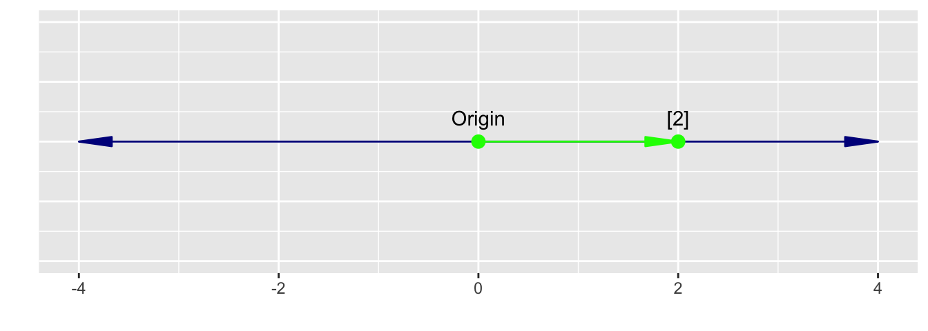
Given a vector with one element: $\overrightarrow{v}=\left[\begin{array}{c}2\end{array}\right]$, this can be thought of as representing a point on a 1-Dimensional number line ranging from $-\mathrm{\infty }\leftarrow 0\to \mathrm{\infty }$ where the element value is the distance from 0.

A one-dimensional vector

We can multiply this vector by any scalar value and get another value on the number line.

This is known as scaling the vector.

Figure A.2: Scaling a one-dimensional vector

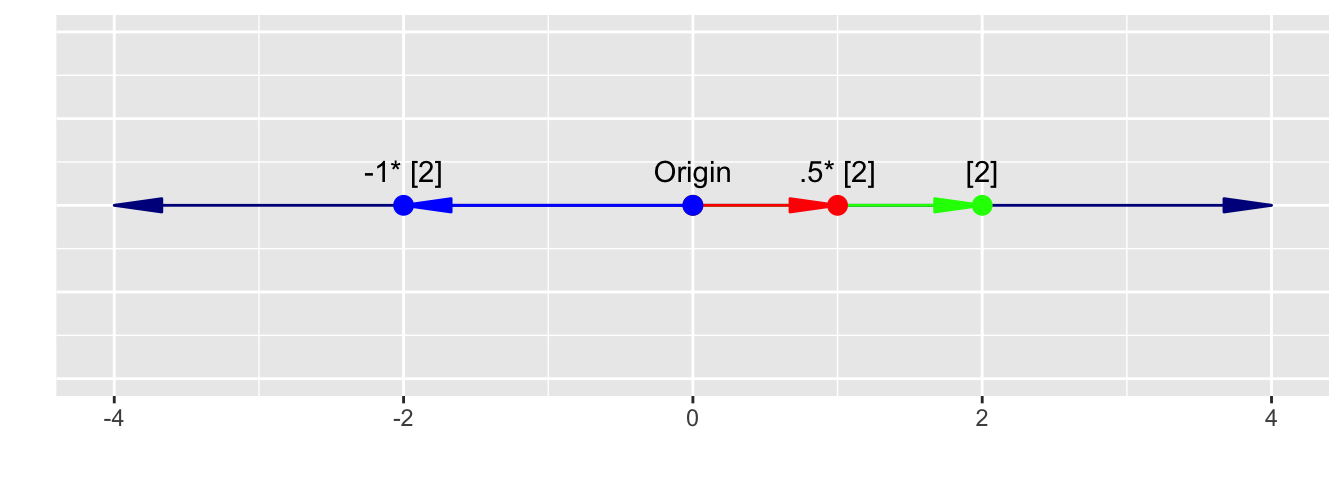
A.11.1.1 The 1-d Unit Vector

We can represent any point on the number line by scaling a vector of length 1, $\hat{i}$ (known as the unit vector), by the appropriate scalar $a$.

The red vector in Figure A.2 above is a unit vector $\hat{i}=\left[\begin{array}{c}1\end{array}\right]$

A.11.1.2 Linear Combinations of 1-d Vectors

We can also create linear combinations of 1-d vectors by adding them together.

$$\begin{array}{rl}\left[\begin{array}{c}4\end{array}\right]+\left[\begin{array}{c}-2\end{array}\right]& =\left[\begin{array}{c}2\end{array}\right]\\ \\ \left[\begin{array}{c}4\end{array}\right]+\left[\begin{array}{c}-2\end{array}\right]& =4\hat{i}+(-2)\hat{i}=2\hat{i}=2\left[\begin{array}{c}1\end{array}\right]\end{array}$$

Span of a Vector and Basis Vectors

The set of all linear combinations of a vector, say $\hat{i}$, is known as the span of the vector.

In 1-d, the span of $\hat{i}$ includes every point on the number line. We don’t need any other vector to find a point.

Thus $\hat{i}$ is known as a generator for the 1-d vector space.

Since there is only 1 vector, $\hat{i}$, in the set of generators for 1-d space, we do not have to check if it is independent of other vectors.

The set of vectors $S$ that are linearly independent and generate the space (their span includes every point in the space) is known as the basis for the space. The member vectors of $S$ are the basis vectors for the space.

Here, $\hat{i}$ is a basis vector for the 1-d vector space.

Vector Space

A vector space of dimension $d$ is a subset of possible values for a geometric object of $d$ dimensions that passes through the origin which has the following properties.

• One can do addition and scalar-multiplication operations
• Those operations are commutative and distributive
• The subset contains the zero vector 0 (the origin).
• If the subset contains $\overrightarrow{v}$ then it contains $a\overrightarrow{v}$ for every scalar $a$.
• If subset contains $\overrightarrow{u}$ and $\overrightarrow{v}$, then it contains $\overrightarrow{u}+\overrightarrow{v}$.

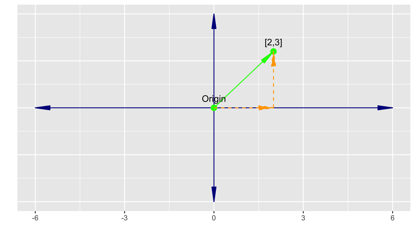
A.11.2 Vectors with Two Elements:${\mathbb{R}}^2$

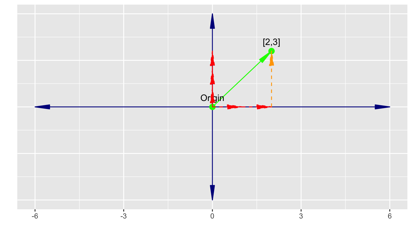
Let’s consider a vector with two elements: $\overrightarrow{v}=\left[\begin{array}{c}2\\ 3\end{array}\right]$.

With two elements, this can be thought of as representing a point on a 2-dimensional $x,y$ plane where both $x$ and $y$ have the range $-\mathrm{\infty }\leftarrow 0\to \mathrm{\infty }$.

• The element values are the distance from 0 in the $x$ direction and then the $y$ direction.
• We use the following notation to denote the $x$ and $y$ elements of the 2 dimensional vector.

$$\overrightarrow{v}=\left[\begin{array}{c}x\\ y\end{array}\right]$$ - The point $(0,0)$ is called the origin. - We will think of all vectors as being expressed geometrically as an arrow with the tail at the origin and head at the point away from the origin.

Figure A.3: A two-dimensional vector

We can still scale a two dimensional vector by multiplying it by a scalar.

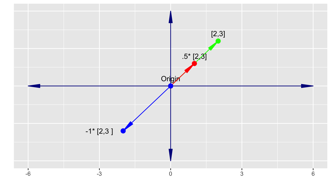
Important

However, we cannot create every point in the 2-d space with one vector, only those points in the span of the original vector.

A single vector does not have a span that generates a 2-d space.

To generate the 2-d space, we need a second vector that is not in the span of the first vector.

A.11.2.1 Unit Vectors in 2-d

Let’s define two unit vectors, ${\overrightarrow{v}}_i$ in the $x$ direction, and ${\overrightarrow{v}}_j$ in the $y$ direction.

$${\overrightarrow{v}}_i=\left[\begin{array}{c}1\\ 0\end{array}\right]\text{ and }{\overrightarrow{v}}_j\left[\begin{array}{c}0\\ 1\end{array}\right]$$

A.11.2.2 Scaling and Vector Addition in 2-d

We can consider the vector $\overrightarrow{v}=\left[\begin{array}{c}2\\ 3\end{array}\right]$ as representing scalar multiplication of two unit vectors, ${\overrightarrow{v}}_i$ in the $x$ direction and ${\overrightarrow{v}}_j$ in the $y$ direction, followed by their addition.

$$\overrightarrow{v}=\left[\begin{array}{c}2\\ 3\end{array}\right]=2{\overrightarrow{v}}_i+3{\overrightarrow{v}}_j=2\left[\begin{array}{c}1\\ 0\end{array}\right]+3\left[\begin{array}{c}0\\ 1\end{array}\right]$$

Figure A.4: A 2-d vector expressed as scaled unit vectors added together.

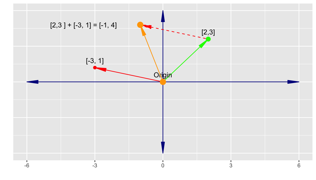
The orange line in Figure A.4 represents the addition of two vectors as discussed in Section A.3.2.

Geometrically, it can be seen as moving the tail of the second vector to the head of the first vector. Their sum is the new location of the head of the second vector.

Let’s add $\overrightarrow{v}=\left[\begin{array}{c}2\\ 3\end{array}\right]+\overrightarrow{v}=\left[\begin{array}{c}-3\\ 1\end{array}\right]$.

• We plot the two vectors with tails at the origin and then move the second (red) vector so its tail is at the head of the first vector.
• The result is the head of the shifted second vector, here

$$\overrightarrow{v}=\left[\begin{array}{c}2\\ 3\end{array}\right]+\left[\begin{array}{c}-3\\ 1\end{array}\right]=\left[\begin{array}{c}-1\\ 4\end{array}\right]$$.

Figure A.5: Addition of 2-d vectors.

A.11.2.3 Linear Combinations and Linear Independence

With two 2-d vectors, $\overrightarrow{u}$ and $\overrightarrow{v}$, we can use scaling and vector addition to create a new vector $\overrightarrow{w}$ that is a linear combination of $\overrightarrow{u}$ and $\overrightarrow{v}$, such that

$$a\overrightarrow{u}+b\overrightarrow{v}=\overrightarrow{w}$$

Every vector space contains the origin.

If $a=b=0$ in $a\overrightarrow{u}+b\overrightarrow{v}=\overrightarrow{w}$, then $\overrightarrow{w}$ is the origin.

Assuming $a,b\ne 0$, then we say $\overrightarrow{u}$ and $\overrightarrow{v}$ are linearly dependent if we can choose $a$ and $b$ such that $a\overrightarrow{u}+b\overrightarrow{v}=0$.

Important

If two vectors are linearly dependent, it means they share the same span. Thus the dimension of the span of the set $\{\overrightarrow{u},\overrightarrow{v}\}$ is 1, not 2.

Consider $\overrightarrow{u}=\left[\begin{array}{c}2\\ 3\end{array}\right]$ and $\overrightarrow{v}=\left[\begin{array}{c}-1\\ -1.5\end{array}\right]$.

• We can find scalars $a=1,b=2$ such that $a\overrightarrow{u}+b\overrightarrow{v}=\overrightarrow{0}$.

$$a\left[\begin{array}{c}2\\ 3\end{array}\right]+b\left[\begin{array}{c}-1\\ -1.5\end{array}\right]⟹\left[\begin{array}{c}2\\ 3\end{array}\right]+2\left[\begin{array}{c}-1\\ -1.5\end{array}\right]=\left[\begin{array}{c}0\\ 0\end{array}\right]$$

• Thus $\overrightarrow{u}$ and $\overrightarrow{v}$ are linearly dependent and share the same span as seen here.

Figure A.6: Two linear dependent vectors have the same span and cannot generate the 2-d space.

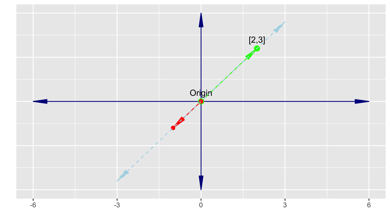
Reducing the span by one dimension from 2-1 is equivalent to converting the vector space from a 2-d plane to a 1-d number line.

To generate a 2-d space, we need a second vector that is not in the span of the first vector i.e., is linearly independent of the first vector.

The unit vectors $\hat{i}$ and $\hat{j}$ are linearly independent.

Thus the set $S=\{\hat{i},\hat{j}\}$ has dimension 2 and can generate the 2-d space.

The set $S=\hat{i},\hat{j}$ are a basis for the 2-d space.

A.11.2.4 Basis Vectors

Is the set $S=\hat{i},\hat{j}$ the only set of basis vectors in 2-d space? No.

Any set of two linearly independent vectors $\overrightarrow{u}$ and $\overrightarrow{v}$, such as $\overrightarrow{u}=\left[\begin{array}{c}2\\ 3\end{array}\right]$ and $\overrightarrow{v}=\left[\begin{array}{c}-1\\ 3\end{array}\right]$, can serve as the basis.

• The vectors do not even have to be orthogonal.

Changing the basis is equivalent to changing the reference coordinate system for the space.

• Any time we interpret the values of the elements in a vector, we are implicitly using the bases vectors to shape our interpretation.

Thus we normally assume we are using $S=\hat{i},\hat{j}$ as the basis since it corresponds to the 2-d Cartesian plane with $x$ as the horizontal axis and $y$ as the vertical axis.

A.11.3 Three dimensions and Higher: ${\mathbb{R}}^n$

The same concepts from ${\mathbb{R}}^1$ and ${\mathbb{R}}^2$ apply as we move into higher dimensions.

A.11.3.1 Vector Elements

For three dimensions ${\mathbb{R}}^3$, a vector now has three elements $\overrightarrow{u}=\left[\begin{array}{c}x\\ y\\ z\end{array}\right]$

For $n$ dimensions, a vector has $n$ elements $\overrightarrow{x}=\left[\begin{array}{c}{x}_1\\ ⋮\\ x_n\end{array}\right]$.

A.11.3.2 Span and Bases in ${\mathbb{R}}^n$

With two linearly independent vectors in 3-d vector space, their span is still in 2-d space.

• In 3-d space, graphing the result of every linear combination of 2 linearly independent vectors, e.g., $a\hat{i}+b\hat{j}=\overrightarrow{w}$, creates a 2-d plane in 3-d space, centered on the origin.
• In ${\mathbb{R}}^n$, the result of every linear combination of $(n-1)$ linearly independent vectors $a_1{\overrightarrow{x}}_1+a_2\overrightarrow{x_2}+\cdots +a_{(n-1)}{\overrightarrow{x}}_{n-1}={\overrightarrow{w}}_{n-1}$ creates an $(n-1)$-dimensional hyper-plane in ${\mathbb{R}}^n$ space, centered on the origin.

If we add a third vector in ${\mathbb{R}}^3$ we can add vectors as before.

• Add the first two vectors by moving the tail of the second to the head of the first.
• Then, move the tail of the third vector to the head of the second.
• The new location of the head of the third vector is the result.

This is equivalent to:

$$\text{Given }\overrightarrow{u}=\left[\begin{array}{c}{x}_1\\ y_1\\ z_1\end{array}\right]\overrightarrow{v}=\left[\begin{array}{c}{x}_2\\ y_2\\ z_2\end{array}\right]\overrightarrow{w}=\left[\begin{array}{c}{x}_3\\ y_3\\ z_3\end{array}\right]$$

$$\begin{gathered} \text{Vector addition } \\ \overrightarrow{u}+\overrightarrow{v}+\overrightarrow{w}=\left[\begin{array}{c}{x}_1+x_2\\ y_1+y_2\\ z_1+z_2\end{array}\right]+\left[\begin{array}{c}{x}_3\\ y_3\\ z_3\end{array}\right]=\left[\begin{array}{c}{x}_1+x_2+x_3\\ y_1+y_2+y_3\\ z_1+z_2+z_3\end{array}\right]=\overrightarrow{w} \end{gathered}$$

The span of the three 3-d vectors is the set $S$ of all possible linear combinations of $a\overrightarrow{u}+b\overrightarrow{v}+c\overrightarrow{w}$.

• The dimension of the $S$ is the number of linearly independent vectors in $S$.
• If one or more of the vectors in $S$ is linearly dependent on one or more of the others, (it is in the span of one or their linear combination), the dimension of set $S$ is still the number of linearly independent vectors in $S$, so may be 1 or 2.
• If the three vectors are all linearly independent of each other, the span of $S$ has dimension 3, the three vectors can generate ${\mathbb{R}}^3$, and the set $S$ can serve as a basis for ${\mathbb{R}}^3$.
• This can be thought of as taking the span of the first two vectors (a horizontal $x,y$ plane) and using the third vector to move it from $-\mathrm{\infty }\to \mathrm{\infty }$ in the $z$ dimension.

In ${\mathbb{R}}^n$, the span of $n$, $n$-dimensional vectors is the set $S$ of all possible linear combinations of $a_1\overrightarrow{x_1}+a_2\overrightarrow{x_2}+\cdots +a_n\overrightarrow{x_n}$.

• The dimension of a set of vectors $S$ is the number of linearly independent vectors in $S$.
• If one or more of the vectors in $S$ is linearly dependent on one or more of the others, (it is in the span of one or a linear combination of others), the dimension of set $S$ is still the number of linearly independent vectors in $S$, so may from range from 1 to $n-1$.
• If the $n$ vectors are all linearly independent of each other, the span of $S$ has dimension $n$, the $n$ vectors can generate ${\mathbb{R}}^n$, and the set $S$ can serve as a basis for ${\mathbb{R}}^n$.

In ${\mathbb{R}}^n$, consider the set of $n$ unit vectors along each axis as the basis for the ${\mathbb{R}}^n$. This helps with the interpretation of matrices as linear transformations of a vector in ${\mathbb{R}}^n$.

A.12 Matrices as Linear Transformations of Vectors

A.12.1 Linear Transformations in General

A transformation is a function that maps an input value to an output value.

We are interested in using a function to map a vector to a different vector in ${\mathbb{R}}^n$.

• The function can be considered the rules for reshaping and moving the input vector to look like the output vector.
• This is equivalent to applying a function to a point in ${\mathbb{R}}^n$ to produce another point in ${\mathbb{R}}^n$.

To make the transformation linear, we have to add two constraints to the function.

1. It must preserve the linearity of lines - all input lines must be output as lines.
2. The origin must not be shifted.

These are equivalent to transformations that keep all the gird lines on the plan as parallel and evenly spaced.

Important

A linear transformation of any $n$ dimensional vector can be described as a linear combination of the unit vectors in the basis for ${\mathbb{R}}^n$.

An example in ${\mathbb{R}}^2$.

• Start with a vector $\overrightarrow{u}=\left[\begin{array}{c}-1\\ 2\end{array}\right]=-1\hat{i}+2\hat{j}$

If we use transformation that moves the vector to $\overrightarrow{v}$, it preserves the coefficients of the linear combination and we just have to think about what happens to the $\hat{i}$ and $\hat{j}$.

$$\overrightarrow{v}=-1(\text{transformed }\hat{i})+2(\text{transformed }\hat{j})$$

If our transformation moved $\hat{i}$ to $\left[\begin{array}{c}1\\ -2\end{array}\right]$ and $\hat{j}$ to $\left[\begin{array}{c}3\\ 0\end{array}\right]$, then the final vector will be

$$\overrightarrow{v}=-1\left[\begin{array}{c}1\\ -2\end{array}\right]+2\left[\begin{array}{c}3\\ 0\end{array}\right]=\left[\begin{array}{c}5\\ 2\end{array}\right]$$

We can write this transformation in terms of any input as

$$\overrightarrow{u}=\left[\begin{array}{c}x\\ y\end{array}\right]\text{transformed }\to x\left[\begin{array}{c}1\\ 2\end{array}\right]+y\left[\begin{array}{c}3\\ 0\end{array}\right]=\left[\begin{array}{c}1x+3y\\ -2x+0y\end{array}\right]$$

We can make this even more general.

Linear Transformations in ${\mathbb{R}}^2$.

We can describe any linear transformation in ${\mathbb{R}}^2$ using just 4 numbers.

• Two for the vector where $\hat{i}$ lands after the transformation and
• Two for the vector where $\hat{j}$ lands after the transformation.

We combine these four numbers (two vectors) into a 2x2 matrix as

$$\left[\begin{array}{c}{x}_{\hat{i}}{x}_{\hat{j}}\\ y_{\hat{i}}{y}_{\hat{j}}\end{array}\right]$$

Where the first column describes the new location of $\hat{i}$ and the second column in the new location of $\hat{j}$.

So, to apply a transformation matrix to any vector in ${\mathbb{R}}^2$, we use the elements in the input vector to create a linear combination of the vectors in the transformation matrix.

Given a 2x2 matrix $\left[\begin{array}{c}32\\ -21\end{array}\right]$, if we want to transform $\left[\begin{array}{c}5\\ 7\end{array}\right]$, the linear combination looks like:

$$\left[\begin{array}{c}32\\ -21\end{array}\right]\left[\begin{array}{c}5\\ 7\end{array}\right]=5\left[\begin{array}{c}3\\ 2\end{array}\right]+7\left[\begin{array}{c}2\\ 1\end{array}\right]=\left[\begin{array}{c}29\\ 17\end{array}\right]$$

Or in general.

$$\left[\begin{array}{c}ab\\ cd\end{array}\right]\left[\begin{array}{c}x\\ y\end{array}\right]=x\left[\begin{array}{c}a\\ c\end{array}\right]+y\left[\begin{array}{c}b\\ d\end{array}\right]=\left[\begin{array}{c}ax+by\\ cx+dy\end{array}\right]$$

Note

Putting the matrix on the left of the vector is equivalent to using $f(\overrightarrow{v})=\overrightarrow{w}$ where $f()$ is a transformation function.

We have previously seen $f()$ as the function for matrix multiplication in Section A.3.4.

A square matrix of size $n$ can thus be interpreted as just a function to make a linear transformation of a vector in ${\mathbb{R}}^n$.

• The linear transformation is completely described by $n^2$ numbers which describe the new locations of the unit vectors in the basis of the space.
• We can put these numbers into the columns of a square matrix to describe where each of the $n$ unit vectors winds up after the transformation.
• Matrix multiplication can be interpreted as reshaping the space to move the input vector into a new position in ${\mathbb{R}}^n$.

A.12.2 Executing Multiple Transformations

We often want to execute a sequence of transformations, sometimes called creating a composition of transformations.

This is equivalent to multiplying multiple matrices.

Since each multiplication results in a new matrix describing where each of the $n$ unit vectors winds up after the transformation, we can just repeat the process.

Note

When multiplying a vector by two matrices, we write it in the form from left to right as

$$\left[\begin{array}{c}ef\\ gh\end{array}\right]\left[\begin{array}{c}ab\\ cd\end{array}\right]\left[\begin{array}{c}x\\ y\end{array}\right]$$

where we execute as $g(f(\overrightarrow{X}))$

$$\left[\begin{array}{c}ef\\ gh\end{array}\right]\left(\left[\begin{array}{c}ab\\ cd\end{array}\right]\left[\begin{array}{c}x\\ y\end{array}\right]\right)$$

As noted in Section A.3.4.3, compositions of matrix transformations (multiple multiplications) are not commutative.

That means, that except for special cases,

$$\left[\begin{array}{c}ef\\ gh\end{array}\right]\left(\left[\begin{array}{c}ab\\ cd\end{array}\right]\left[\begin{array}{c}x\\ y\end{array}\right]\right)\ne \left[\begin{array}{c}ab\\ cd\end{array}\right]\left(\left[\begin{array}{c}ef\\ gh\end{array}\right]\left[\begin{array}{c}x\\ y\end{array}\right]\right)$$

A.12.3 Determinants

These linear transformations by matrices are reshaping the space of the input vector.

This means they are often either stretching the space or shrinking the space, with or without some rotations in one or more dimensions.

In ${\mathbb{R}}^2$, we are often then interested in by what factor does a transformation change the area of a space.

Consider the transformation matrix $\left[\begin{array}{c}30\\ 02\end{array}\right]$.

• It scales $\hat{i}$ by a factor of 3 and $\hat{j}$ by a factor of 2.
• This means that the 1 x 1 square formed by $\hat{i}$ and $\hat{j}$ now is a 3 x 2 rectangle so has an area of 6.
• We can say this linear transformation scaled the area by a factor of 6.

Figure A.7: A linear transformation can scale the area of the 2-d space.

Now, consider a linear transformation known as a shear transformation.

• It has the transformation matrix $\left[\begin{array}{c}11\\ 01\end{array}\right]$
• This leaves $\hat{i}$ in place but moves $\hat{j}$ over to $(1,1)$.
• This means the 1 x 1 square is now a parallelogram but it still has area 1.

Figure A.8: A linear shear transformation scales the area of the 2-d space into a parallelogram.

This scaling factor of a linear transformation matrix is called the determinant of the transformation matrix as seen back in Section A.2.1.1.

• This scaling factor applies to any area defined by vectors in ${\mathbb{R}}^2$.

• For ${\mathbb{R}}^n$, the matrix will scale the volumes instead of the area.

• For ${\mathbb{R}}^{n}3$, it is the volume of the parallelepiped created by the three unit vectors along each axis.

• If $A$ is a transformation matrix with determinant 3, it scales up all the areas by a factor of 3.

• If $B$ is a transformation matrix with determinant 1/2, it shrinks down all the areas by a factor of 1/2.

Determinant of 0

If a 2-d transformation matrix has a determinant of 0, it shrinks all of the space into a 1-d line or even a single point (0,0).

This is equivalent to the columns of the matrix being linearly dependent.

This can be useful as we will see later on to simplify the representation of a transformation as a matrix.

What does it mean to have a determinant that is $<0$?

• This is known as a transformation that flips the coordinate reference system or “invert the orientation of space”.
• This can also be visualized as $\hat{i}$ moving from the usual position to the right of $\hat{j}$ to now being on the left of $\hat{j}$.
• The Absolute Value of the determinant still shows how much the areas have been scaled (increased or shrunk down).
• In ${\mathbb{R}}^3$, this means the orientation has been inverted from a “right hand rule” to a “left-hand rule”.

To take a general view, consider the matrix $A=\left[\begin{array}{c}ab\\ cd\end{array}\right]$ where

$$\text{det}(A)=\text{det}\left(\left[\begin{array}{c}ab\\ cd\end{array}\right]\right)=ad-bc$$

If $b=c=0$ then there then $A$ is the diagonal matrix $A=\left[\begin{array}{c}a0\\ 0d\end{array}\right]$.

• The transformation creates a new rectangle out of the unit vector 1x1 square as seen in Figure A.7.
• $a$ is the factor for how much $\hat{i}$ is stretched.
• $b$ is the factor for how much $\hat{j}$ is stretched
• $ab$ is the area of the new rectangle compared to the original 1x1 square.

If either $b$ or $c$ is non-zero, then,

• The transformation creates a new parallelogram out of the unit vector 1x1 square as seen in Figure A.8.
• $ab$ is still the area of the new parallelogram, with base $a$ and height $b$, compared to the original 1x1 square.

If $b$ and $c$ are both non-zero, then,

• The transformation creates a new parallelogram out of the unit vector 1x1 square and stretches (shrinks) it in the diagonal direction.

Note

When multiplying two matrices, $A$ and $B$, $\text{det}(AB)=\text{det}(A)\text{det}(B)$

A.13 Matrices and Systems of Linear Equations

A system of linear equations is a set of equations that describes the relationships among $n$ variables through scaling the variables and adding then together to create a result.

We want to solve the system of linear equations and transformation matrices can help us do that.

If you have a system of linear equations you can organize it with all of the variables and their coefficients on the left and all of the results (scalars) on the right of the equal sign.

• You may need to make $0$ or $1$ coefficients explicit so you have the same number of coefficients in each equation.

Now, convert the system of equations into matrix form by converting the variables and results to vectors and the coefficients into a matrix.

$$\begin{array}{rl}2x+5y+3z& =-3\\ 4x+0y+8z& =0\\ 1x+3y+0z& =2\end{array}\to \left[\begin{array}{c}253\\ 408\\ 130\end{array}\right]\stackrel{\text{Variables}}{\overbrace{\left[\begin{array}{c}x\\ y\\ z\end{array}\right]}}=\left[\begin{array}{c}-3\\ 0\\ 2\end{array}\right]$$

We can label each part as follows

$$\begin{array}{rl}2x+5y+3z& =-3\\ 4x+0y+8z& =0\\ 1x+3y+0z& =2\end{array}\to \stackrel{A}{\overbrace{\left[\begin{array}{c}253\\ 408\\ 130\end{array}\right]}}\stackrel{\overrightarrow{x}}{\overbrace{\left[\begin{array}{c}x\\ y\\ z\end{array}\right]}}=\stackrel{\overrightarrow{v}}{\overbrace{\left[\begin{array}{c}-3\\ 0\\ 2\end{array}\right]}}$$

and now rewrite in matrix vector form:

$$\begin{array}{}\text{(A.7)}& A\overrightarrow{x}=\overrightarrow{v}\end{array}$$

We can interpret the system of equations then as a matrix transformation (or function) of the input vector $\overrightarrow{x}$ that results in the vector $\overrightarrow{v}$.

Our interest is in figuring out what input vector $\overrightarrow{x}$, when the space is scaled and squished by $A$, now looks like $\overrightarrow{v}$.

There are two cases

1. The matrix $A$ squishes the space down by a dimension, i.e., $\text{det}(A)=0$
2. The matrix $A$ squishes the space in a way that preserves the dimension of the space, i.e., $\text{det}(A)\ne 0$

A.13.0.1 Solutions with $\text{det}(A)\ne 0$

When $\text{det}(A)\ne 0$, there where always be one, and only one, $\overrightarrow{x}$ such that $A\overrightarrow{x}=\overrightarrow{v}$.

We can find this by reversing the transformation. This reverse of the transformation is its own transformation matrix which is called the inverse of $A$ or $A^{-1}$.

As an example, if $A$ were a counterclockwise rotation of ${90}^{\circ }$, $\left[\begin{array}{c}0-1\\ 10\end{array}\right]$ then,

$A^{-1}$ would be the matrix of a clockwise rotation of ${90}^{\circ }$, $\left[\begin{array}{c}01\\ -10\end{array}\right]$.

So in case 2, where $A^{-1}$ exists, like with functions where $f^{-1}f(x)=x$, you wind up where you started.

$$A^{-1}A\overrightarrow{x}=\overrightarrow{x}\text{ and }{A}^{-1}A=I=\left[\begin{array}{c}10\\ 01\end{array}\right]$$

Now we can solve for $\overrightarrow{x}$ by multiplying both sides of Equation A.7 by $A^{-1}$ to get

$$A^{-1}A\overrightarrow{x}=A^{-1}\overrightarrow{v}⟹\overrightarrow{x}=A^{-1}\overrightarrow{v}$$

This can be interpreted as using $\overrightarrow{v}$ as the input vector and shifting its space using $A^{-1}$ to see what vector is the output, the $\overrightarrow{x}$ of interest.

A.13.0.2 Solutions with $\text{det}(A)=0$

When the system of equations has a transformation matrix $A$ with $\text{det}(A)=0$, then the matrix squishes the space down into a volume of 0, effectively dropping the dimension of the space by one.

• $\text{det}(A)=0⟹\nexists A^{-1}$

However, there can still be a solution to the system of equations if the solution exists in the lower dimensional space.

As an example, if a 2-d matrix squishes down to a line, it could be true that $\hat{v}$ is in the span of that line.

In ${\mathbb{R}}^3$, it is also possible for a solution to exist if $A$ squishes down the solution space by 2 dimensions to a plane or even 1 dimension to a line.

• It would much hard to find a solution for the single line than for the plane even though both have $\text{det}(A)=0$.

To differentiate the different types of output in higher dimensions, we use the term Rank.

• If the transformation matrix has an output of 1-d, the matrix has Rank = 1.
• If the transformation matrix has an output of 2-d, the matrix has Rank = 2.
• and so on.

The set of all possible outputs of $A\overrightarrow{v}$ is called the Column Space of $A$.

• You can think about it as the number of columns in $A$ where each represents the effect on the unit vectors.
• The span of these vectors is all possible outputs, which by definition is the column space.
• So, Rank is also the number of dimensions of the column space.
• If a matrix has a Rank = the number of columns, which is as high as it could be, the matrix has Full Rank.

If a matrix has full rank, then the only vector that transforms to the origin is the 0 vector.

If a matrix has less than full rank, so it squishes down to a smaller dimension, then you can have a lot of vectors that transform to 0.

If a 2-d matrix squishes to a line, there is a second line, in a different direction, where all the vectors on the second line, get squished onto the origin.

This set of vectors (or planes in higher dimensions) that transform to the origin, to 0, are called the Null Space or Kernel of the matrix.

Null Space

In a system of linear equations, the Null Space of the matrix $A$ gives all possible solutions to the system when $A\overrightarrow{x}=\overrightarrow{0}$

A.14 Change of Bases

In Section A.11.2.4, we discussed that there many possible basis vectors for a vector space.

The choice of basis vectors determines how to describe other vectors in terms of the origin, the direction of movement and the unit of distance.

As an example, $\hat{i}$ and $\hat{j}$ mean we interpret a vector $\left[\begin{array}{c}3\\ 2\end{array}\right]$ as saying the head of the vector can be found by moving three units horizontally to the right and two units vertically up from the origin.

This relationship between the numbers and a geographic interpretation as a vector is defined by the Coordinate System.

• $\hat{i}$ and $\hat{j}$ are part of a “standard” Coordinate system with length one and horizontal and vertical basis vectors of length 1.

A.14.1 Differing Linear Coordinate Systems

Suppose someone else uses a different set of basis vectors, ${\overrightarrow{b}}_1$ and ${\overrightarrow{b}}_2$ where from the perspective of the standard coordinate system, ${\overrightarrow{b}}_1$ points up to the right at a slight angle, and ${\overrightarrow{b}}_2$ points up to the left at a slight angle.

What the standard system defines as $\left[\begin{array}{c}3\\ 2\end{array}\right]$ would be described as $\left[\begin{array}{c}5/3\\ 1/3\end{array}\right]$ in the system with basis vectors ${\overrightarrow{b}}_1$ and ${\overrightarrow{b}}_2$.

Important

The original vector has not moved - it is just being described from the perspective of a different coordinate system.

• The origin is the same $\overrightarrow{0}$
• It is the same approach of scaling each basis vector and adding the results.
• However the orientation of the axes and the scaling of the units is different.
• The choice of these is arbitrary and can be changed to provide a more visually or mathematically convenient perspective of a vector.
• Consider a picture taken by a tilted camera and tilting your head a few degrees so it looks like a normal portrait or landscape perspective. The location of objects and the relationships among objects in the picture did not change, but it might be easier to interpret now that your are looking at it from a new perspective.

In this example, the standard coordinate system would describe ${\overrightarrow{b}}_1=\left[\begin{array}{c}2\\ 1\end{array}\right]$ and ${\overrightarrow{b}}_2=\left[\begin{array}{c}-1\\ 1\end{array}\right]$

In the alternate system, ${\overrightarrow{b}}_1=\left[\begin{array}{c}1\\ 0\end{array}\right]$ and ${\overrightarrow{b}}_2=\left[\begin{array}{c}0\\ 1\end{array}\right]$ and are the unit basis vectors.

A.14.2 Translating (Transforming) a Vector Between Coordinate Systems

Given two coordinate systems we can translate a vector from one representation to the other if we can describe the basis vectors in one system in terms of the other.

Assume there is a vector identified as $\left[\begin{array}{c}-1\\ 2\end{array}\right]$ in the alternate system.

What would its description be in the standard coordinate system?

We know how to describe the basis vectors in the alternate system using standard coordinates so we can apply the scale from the alternate system to those.

$$-1\left[\begin{array}{c}2\\ 1\end{array}\right]+2\left[\begin{array}{c}-1\\ 1\end{array}\right]=\left[\begin{array}{c}-4\\ 1\end{array}\right]$$

This is just the same as using the basis vectors of the alternate system, as a transformation matrix to describe the change using the standard coordinate system.

Important

This matrix is called the Change of Basis matrix as it changes $\hat{i}$ and $\hat{j}$ to ${\overrightarrow{b}}_1$ and ${\overrightarrow{b}}_2$.

That is equivalent to changing the description of the vector based on scaling the basis vectors ${\overrightarrow{b}}_1$ and ${\overrightarrow{b}}_2$ to a description using the basis vectors $\hat{i}$ and $\hat{j}$ using the standard coordinate system.

• The change of basis matrix allows us to describe a vector from the alternate system in terms of the standard coordinate system basis vectors $\hat{i}$ and $\hat{j}$.

$$\left[\begin{array}{c}2-1\\ 11\end{array}\right]\left[\begin{array}{c}-1\\ 2\end{array}\right]=\left[\begin{array}{c}-4\\ 1\end{array}\right]$$

To transform from the standard to the alternate just requires using the inverse of the change of basis matrix.

• To translate a standard coordinate vector $\left[\begin{array}{c}3\\ 2\end{array}\right]$, multiply it by the inverse of the change of basis matrix to get the description in terms of scaling the basis vectors ${\overrightarrow{b}}_1$ and ${\overrightarrow{b}}_2$.
• We get the result mentioned earlier.

$${\left[\begin{array}{c}2-1\\ 11\end{array}\right]}^{-1}=\left[\begin{array}{c}1/31/3\\ -1/32/3\end{array}\right]\to \left[\begin{array}{c}1/31/3\\ -1/32/3\end{array}\right]\left[\begin{array}{c}3\\ 2\end{array}\right]=\left[\begin{array}{c}5/3\\ 1/3\end{array}\right]$$

A.14.3 Translating (Transforming) a Matrix Between Coordinate Systems

We can also translate a matrix that describes a transformation for a vector written in one coordinate system so the translated matrix describes the same spatial transformation from the perspective of the basis vectors in the alternate coordinate system.

• This means we can’t just multiply by the coordinate transformation matrix as that would still be describing the transformation in terms of $\hat{i}$ and $\hat{j}$.

Assume we have a transformation matrix $\left[\begin{array}{c}0-1\\ -10\end{array}\right]$ to rotate a vector ${90}^{\circ }$ to the left (counterclockwise) in the standard coordinate system. We want to apply that transformation to a vector in an alternate coordinate system where we know the change of basis matrix is $\left[\begin{array}{c}2-1\\ 11\end{array}\right]$.

The following steps will translate a transformation matrix written in one system so it can describe the same transformation of a vector in an alternate coordinate system by using the change of basis matrix.

1. Start with the vector written in the alternate coordinate system.
2. Translate it to the standard coordinate system using the change of basis matrix.
3. Transform it with the transformation matrix in the standard coordinate system.
4. Translate it back to the alternate system using the inverse of the change of basis matrix.

$$\stackrel{\text{4. Translate to Alternate}}{\overbrace{{\left[\begin{array}{c}2-1\\ 11\end{array}\right]}^{-1}}}\stackrel{\text{3. Transform in Standard}}{\overbrace{\left[\begin{array}{c}0-1\\ -10\end{array}\right]}}\stackrel{\text{2. Translate to Standard (CofB)}}{\overbrace{\left[\begin{array}{c}2-1\\ 11\end{array}\right]}}\stackrel{\text{1. Alternate Basis}}{\overbrace{\overrightarrow{v}}}=\stackrel{\text{ Transform in Alternate}}{\overbrace{\left[\begin{array}{c}1/3-2/3\\ 5/3-1/3\end{array}\right]}}$$

The result of this series of matrix multiplications in the new matrix on the right which will now create the equivalent rotation of ${90}^{\circ }$ left to any vector in the alternate coordinate system based in terms of scaling/shrinking the basis vectors ${\overrightarrow{b}}_1$ and ${\overrightarrow{b}}_2$.

Important

We can now choose to use different coordinate systems, and each system’s set of basis vectors’ and go back and forth in a way that makes it easier to do our analysis.

• This can be thought of as similar to using a log transform to minimize numerical precision errors when multiplying a very large number and and very small small number on a computer.
  • We take the log of each number, add the logged values, and then use the anti-log (or exponentiation) to translate back to the original space to get the final result.

A.15 Eigenvectors and Eigenvalues of a Linear Transformation Matrix

A.15.1 Background

Eigenvectors and their associated eigenvalues have been used in mathematics to “simplify” the analysis of linear transformations since the 18^th century.

• Euler was using linear transformations in ${\mathbb{R}}^3$ to analyze the rotation of solid bodies centered on the origin.
• He found that the linear transformation matrix describing the rotation also rotated most vectors.
• However, the vector of the axis of rotation was special in that it did not rotate under the transformation.
• Another way of saying this is the axis of rotation vector remains on its own span after the transformation and is not rotated off of it like most vectors.
• Others studied these special vectors and determined that many (but not all) matrices of linear transformations may have one or more of these special vectors, which remain on their original span, and which may be scaled by the transformation but not rotated off the span.
• In 1904, David Hilbert coined the term eigenvector (German for “own”) as each transformation matrix may have one or more of its “own” special vectors.
• The eigenvalues are the scale factors associated with one more eigenvectors for a matrix.

Important

When a matrix has a set of eigenvectors that span the space, changing the coordinate system to use them as the basis vectors (an eigenbasis), greatly simplifies the transformation matrix.

• Translating the transformation matrix into the eigenbasis coordinate system translates the original matrix into a diagonal matrix.
• The columns now represent each eigenvector.
• The values on the diagonals are the eigenvalues (scale factors) for each eigenvector!

A.15.2 Example

Let’s assume we have a transformation matrix $\left[\begin{array}{c}31\\ 02\end{array}\right]$.

• We can see from the matrix that $\hat{i}$ is special in that it is not rotated off of its span (the $x$ axis). It is only scaled by a factor of 3.

• Any other vector on the $x$ axis is also scaled by a factor of 3.

• Thus $\hat{i}$ is an eigenvector with eigenvalue 3.

• It turns out the vector $\left[\begin{array}{c}-1\\ 2\end{array}\right]$ is also not rotated off its span and is scaled by a factor of 2.

• An other vector in its span is also not rotated off the span and is just scaled by a factor of 2.

• Thus $\left[\begin{array}{c}-1\\ 2\end{array}\right]$ is an eigenvector with eigenvalue 2.

Important

Using eigenvectors as the basis provides a way of describing a linear transformation that emphasizes the effects of the transformation without worrying about which coordinate system is being used to describe it.

A.15.3 Derivation

Given a transformation matrix $A$, the definition of an eigenvector $\overrightarrow{v}$ is that the output of $A$ transforming $\overrightarrow{v}$ is a scaled version of $\overrightarrow{v}$. That can be expressed as:

$$\begin{array}{}\text{(A.8)}& A\overrightarrow{v}=\stackrel{\text{eigenvalue}}{\overbrace{\lambda }}\overrightarrow{v}\end{array}$$

To find the eigenvectors and eigenvalues of a matrix $A$, we have to solve Equation A.8.

We can do some rearranging to put into a matrix form.

$$\begin{array}{}\text{(A.9)}& \begin{array}{rl}A\overrightarrow{v}& =\lambda \overrightarrow{v}\\ A\overrightarrow{v}& =(\lambda I)\overrightarrow{v}\\ \to \\ A\overrightarrow{v}-(\lambda I)\overrightarrow{v}& =\overrightarrow{0}\\ \to \\ (A-\lambda I)\overrightarrow{v}& =\overrightarrow{0}\end{array}\end{array}$$

The last line in Equation A.9 says we are looking for a vector$\overrightarrow{v}$ such that the new transformation matrix $(A-\lambda I)$ applied to $\overrightarrow{v}$ maps to $\overrightarrow{0}$.

• This means that we are looking for a vector $\overrightarrow{v}\ne \overrightarrow{0}$ that is squished by $(A-\lambda I)$ to $\overrightarrow{0}$.
• That only happens if $\text{det}(A-\lambda I)=0$.

Important

We are thus looking for a $\lambda$ such it causes $(A-\lambda I)$ to be singular with determinant of zero.

As an example, if $A=\left[\begin{array}{c}22\\ 13\end{array}\right]$ the value of $\lambda$ that causes $\text{det}(A-\lambda I)=\text{det}\left(\left[\begin{array}{c}2-\lambda 2\\ 13-\lambda \end{array}\right]\right)=0$ is $\lambda =1$.

• If we had chosen another matrix, the eigenvalue might not be 1.

Since $\text{det}(A-(1)I)=0$ that means there exists a $\overrightarrow{v}\ne \overrightarrow{0}$ where $(A-\lambda I)\overrightarrow{v}=0$ or $A\overrightarrow{v}=(\lambda )\overrightarrow{v}$.

To check if a value of $\lambda$ is an eigenvalue, you can substitute into $\text{det}(A-\lambda I)$ and see if it equals 0.

Using the formula for a 2x2 matrix determinant we can compute $\text{det}\left(\left[\begin{array}{c}3-\lambda 1\\ 02-\lambda \end{array}\right]\right)$ for the original example of $\left[\begin{array}{c}31\\ 02\end{array}\right]$.

• That gives us the following:

$$\text{det}\left(\left[\begin{array}{c}3-\lambda 1\\ 02-\lambda \end{array}\right]\right)=(3-\lambda )(2-\lambda )-0(1)=(3-\lambda )(2-\lambda )=0.$$

This a quadratic polynomial in $\lambda$ where the roots of the polynomial are $3$ and $2$.

To figure out the eigenvectors with these eigenvalues, substitute the eigenvalue back into the $\left[\begin{array}{c}3-\lambda 1\\ 02-\lambda \end{array}\right]$ and compute the vector.

For eigenvalue 2, we get

$$\begin{array}{rl}\left[\begin{array}{c}3-21\\ 02-2\end{array}\right]\left[\begin{array}{c}x\\ y\end{array}\right]& =\overrightarrow{0}\\ \\ \left[\begin{array}{c}11\\ 00\end{array}\right]\left[\begin{array}{c}x\\ y\end{array}\right]& =\overrightarrow{0}\\ \to \\ x+y& =0\\ \to \\ \{x=-1& ,y=1\}\end{array}$$

• So an eigenvector for $\lambda =2$ is $\overrightarrow{v}=\left[\begin{array}{c}-1\\ 1\end{array}\right]$ and any vector in the span of that line, $x=-y$, is a solution for the equation.

Similarly, the eigenvector for $\lambda =3$ we get

$$\begin{array}{rl}\left[\begin{array}{c}3-31\\ 02-3\end{array}\right]\left[\begin{array}{c}x\\ y\end{array}\right]& =\overrightarrow{0}\\ \\ \left[\begin{array}{c}01\\ 0-1\end{array}\right]\left[\begin{array}{c}x\\ y\end{array}\right]& =\overrightarrow{0}\\ \to \\ y& =0\\ \to \\ \{x,y=0\}\end{array}$$

• So an eigenvector for $\lambda =3$ is $\overrightarrow{v}=\left[\begin{array}{c}1\\ 0\end{array}\right]$ and any vector in the span of that line, $y=0$, is a solution for the equation.

Note

Note not every matrix has eigenvectors.

A rotation of ${90}^{\circ }$in ${\mathbb{R}}^2$ by definition rotates every vector off of its span.

• The transformation matrix is $\left[\begin{array}{c}0-1\\ 10\end{array}\right]$ and the roots of $\text{det}(A-\lambda I)=0$ are the roots of $(-\lambda )(-\lambda )=-1$ so the roots are the complex numbers $\pm i$.
• Having only complex roots means there are no eigenvectors in ${\mathbb{R}}^n$.

For a shear transformation in ${\mathbb{R}}^2$, the only eigenvector is $\hat{i}$ with eigenvalue 1. But $\hat{i}$ does not generate ${\mathbb{R}}^2$ so you can’t have an eigenbasis.

A.15.4 Eigenbases

Assume we have a transformation matrix in ${\mathbb{R}}^2$ with two eigenvectors that span the space, say ${\overrightarrow{v}}_1=\left[\begin{array}{c}-1\\ 0\end{array}\right]$ and ${\overrightarrow{v}}_2=\left[\begin{array}{c}0\\ 2\end{array}\right]$.

Putting this into a transformation matrix, we have $\left[\begin{array}{c}-10\\ 02\end{array}\right]$ which is a diagonal matrix.

Diagnonal Matrices and Eigenvectors and Eigenvalues

Any time we have a diagonal matrix, where all off diagonal values = 0, we can interpret this as the matrix of an eigenbasis where each column is an eigenvector with an eigenvalue of the diagonal element for that column.

Diagonal matrices are often easier to work with than non-diagonal matrices.

• As an example, raising a diagonal matrix to the power $n$ simply requires raising the diagonal values to the power $n$ and multiplying the vector.

If you have a transformation that has sufficient eigenvectors to create an eigenbasis, you can change to the eigenbasis to make your computations and then change back as desired as seen in Section A.14.3.

Follow similar steps.

1. Take the original transformation
2. Put the eigenvectors into a change of basis matrix and put that on the right.
3. Put the inverse of the eigenvector change of basis matrix on the left.

The resulting matrix is guaranteed to be diagonal which may make the computations easier.

A.15.5 Beyond Matrices

The concepts of eigenvectors and eigenvalues have been looked at from the perspective of matrices which represent linear transformations.

These matrices are functions that map an input vector to an output vector in ${\mathbb{R}}^n$.

The concepts of eigenvectors and eigenvalues can be extended to operate in other functions that express linear transformation.