           Murder Assault UrbanPop Rape
Alabama      13.2     236       58 21.2
Alaska       10.0     263       48 44.5
Arizona       8.1     294       80 31.0
Arkansas      8.8     190       50 19.5
California    9.0     276       91 40.6
Colorado 7.9 204 78 38.710 Unsupervised Learning Methods
10.1 Unsupervised Learning
Supervised Learning, with labeled data, allows us to check our models. While we don’t know the exact true nature of the relationship, we do know some true results.
Unsupervised learning uses unlabeled data. We don’t know the true results.
Unsupervised learning is often about “exploring the data” to find relationships that might help us understand.
- We have to be careful if relationships that emerge are “true” or just artifacts of the noise in the data.
10.2 Principal Components Analysis (PCA) Review
PCA was an unsupervised method where we were looking to find relationships among the \(X\) that would allow us to reduce multicollinearity among the predictors and reduce the dimension of our model.
We used PCA for Principal Components Regression (PCR) where we were willing to trade off a little bias for a reduction in the variance of our parameter estimates by using \(K < p\) predictors that captured “most” of the variance in \(Y\).
Recall we determined that scaling the predictors is important in PCR when we have wide ranges in the magnitudes of the predictors.
10.3 Clustering Methods (12.4)
Clustering is a broad set of unsupervised methods for trying to determine which observations are “similar” to each other based on the variables in the data.
We will use a measure of “similarity” to identify subgroups where the observations in a subgroup are more similar to each other than to members of other subgroups.
We are trying to find the groups that are most homogeneous
These methods can differ based on how they measure “similar” and the purpose of the analysis.
A very popular method is \(K\)-means Clustering where you first determine how many subgroups you think are appropriate, \(K\), and then try to find the \(K\) subgroups within the observations.
A second popular method is Hierarchical Clustering where you aggregate observations together until you have created clusters of size 1 to size \(n\) and then you determine how many clusters are appropriate.
Concept: We want to maximize the distance between clusters (sub-groups) while minimizing the distances between points within each cluster in \(p\) dimensional space.
- We could make each point its own cluster, but that has not simplified anything.
Goal: For a given \(K\), assign each point to one \(K\) clusters to minimize the following objective function based on the weighted sum of the distance between each point in a cluster:
\[ \sum_{k=1}^{K} \frac{1}{\underbrace{|C_k|}_\text{size, points in cluster k}}\sum_{i, j \in C_k}\underbrace{||X_i - X_j||^2}_\text{L2 Norm for Distance} \]
This will help us create clusters that are the most dense, with the points in each cluster closest to each other.
How do we solve this? Exhaustive Search?
- If we have a sample of size \(n\), how many ways can we split it?
- There are \(\sim K^n\) possible choices, so infeasible for any reasonable data set.
Two popular methods use Sequential Search get a “local optima” as it requires much less computation than finding the true “global optima”.
- Hierarchical Clustering
- \(K\)-means Clustering
10.4 Hierarchical Clustering
Concept: Build an upside-down tree starting with \(n\) leaves on the bottom and create clusters (branches) as we work our way up to from the leaves to build a hierarchy of similar observations within clusters.
We have to make two choices:
- A measure for distance, here we are using the \(L_2\) Norm but others are possible.
- A method for determining the “linkage” between the clusters so we can calculate their “dissimilarity”.
- Four common linkages: Complete, Single, Average, and Centroid of which Average and Complete are generally preferred.
- There are many others.
- The linkage can affect the shape of the clusters in \(p\) space.
An Algorithm
- Start with each observation as its own cluster - a leaf node.
- Calculate the distances between every pair of clusters i.e., \(n\choose{2}\) \(= \frac{n(n-1)}{2}\) of \(O(n^2)\) calculations.
- Calculate the chosen dissimilarity among the clusters by computing all pairwise distances between observations in cluster A and observations in cluster B and then choosing the appropriate value for dissimilarity based on the chosen “linkage”. If there are 3 observations in cluster A and 2 in cluster B there will be 6 measurements. Use a linkage such as the following to get the dissimilarity value for (A, B).
- For Complete (Maximal Inter-cluster dissimilarity) take the Largest distance.
- For Average (Mean Inter-cluster dissimilarity) take the Average of the distances.
- Merge the two clusters with the smallest dissimilarity (most similar; the closest) into a cluster.
- Repeat steps 2-4 until only one cluster remains (as the root node).
The height of the branches from one set of clusters to their joined (or fused) cluster is based on the chosen dissimilarity.
- The greater the sum of the branches between two clusters to their fused or common cluster, the more dissimilar the two clusters.
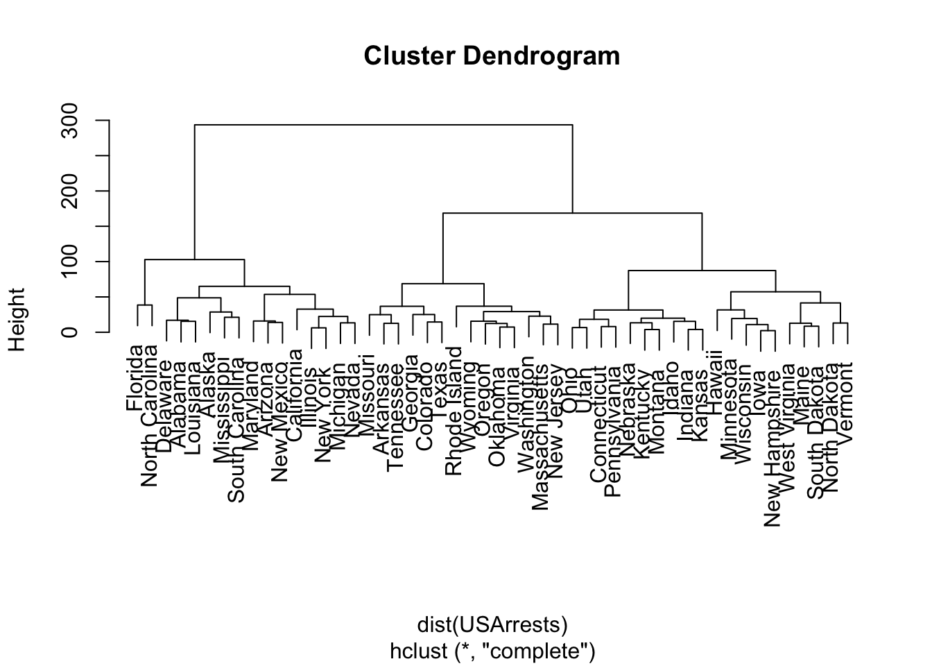
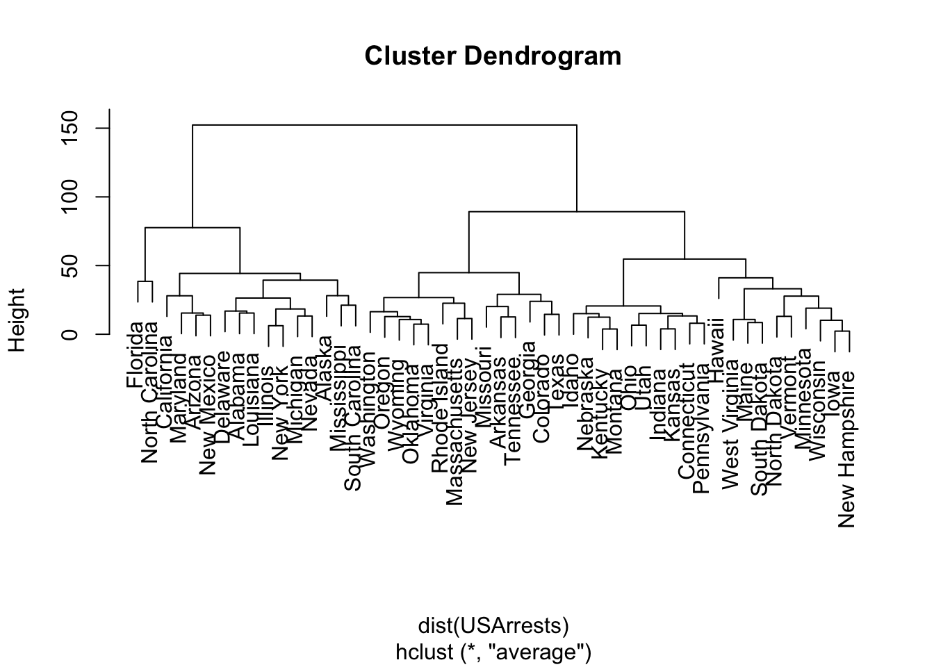
Now that you have a tree (known as a dendrogram- “tree figure drawn by math”), you can choose the number of clusters you think appropriate by make a horizontal slice across the tree.
- The number of branches you cut with the horizontal line determines the number of clusters.
10.4.1 Example of Hierarchical Clustering in R with USArrests Data
Let’s use a small data set, datasets::USArrests.
- This data set contains statistics, in arrests per 100,000 residents for assault, murder, and rape in each of the 50 US states in 1973. Also given is the percent of the population living in urban areas.
- The states are row labels and not predictors so all the data is of class numeric.
We use stats::hclust() for hierarchical clustering.
-
dist()first produces a distance matrix across all the points.- The default is the \(L_2\) or euclidean norm.
- Here that means for two observations (Alabama and Alaska), \(\text{dist}(\text{AL, AK}) = \sum_{i=1}^4(USArrests[1, i] - USArrests[2, i])^2\)
- This produces a lower triangular matrix of the distance between each state.
- If you have mixed classes of data, consider the {cluster} package to compute distance
-
method = "complete"is the default agglomeration method forhclust.
Call:
hclust(d = dist(USArrests))

Cluster method   : complete
Distance         : euclidean
Number of objects: 50
We can plot the dendrogram (with plot.hclust()).
Let’s cut the tree to five clusters with stats::cutree() which produces a named vector of the clustered points.
       Alabama         Alaska        Arizona       Arkansas     California
             1              1              1              2              1
      Colorado    Connecticut       Delaware        Florida        Georgia
             2              3              1              4              2
        Hawaii          Idaho       Illinois        Indiana           Iowa
             5              3              1              3              5
        Kansas       Kentucky      Louisiana          Maine       Maryland
             3              3              1              5              1
 Massachusetts       Michigan      Minnesota    Mississippi       Missouri
             2              1              5              1              2
       Montana       Nebraska         Nevada  New Hampshire     New Jersey
             3              3              1              5              2
    New Mexico       New York North Carolina   North Dakota           Ohio
             1              1              4              5              3
      Oklahoma         Oregon   Pennsylvania   Rhode Island South Carolina
             2              2              3              2              1
  South Dakota      Tennessee          Texas           Utah        Vermont
             5              2              2              3              5
      Virginia     Washington  West Virginia      Wisconsin        Wyoming
             2              2              5              5              2
We can see that each state has a cluster number.
With table() we can see how many are in each cluster.
HC5
 1  2  3  4  5
14 14 10 2 10 Murder Assault UrbanPop Rape
Florida 15.4 335 80 31.9
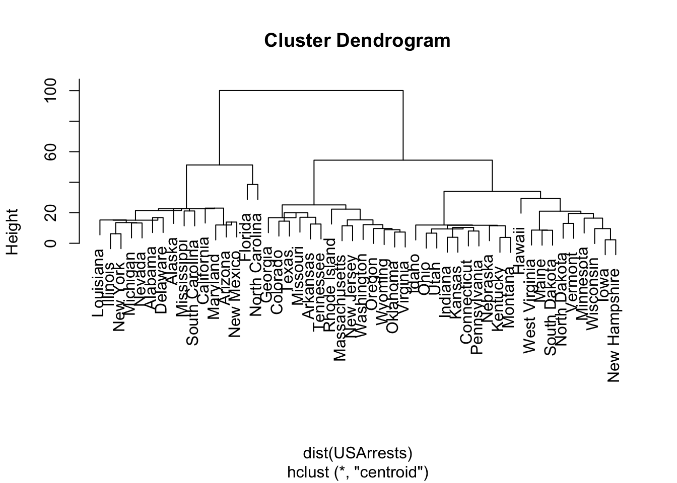
North Carolina 13.0 337 45 16.1What if we used a different method, say centroid?
HCC5
 1  2  3  4  5
14 14 20 1 1 Florida North Carolina
4 5 We get a different hierarchy. If we used “average” we get the same tree as “Complete”.
HCA5
 1  2  3  4  5
14 14 10 2 10 HC5 HCA5 HCC5
Hawaii 5 5 3
Idaho 3 3 3
Illinois 1 1 1
Indiana 3 3 3
Iowa 5 5 3
Kansas 3 3 3
Kentucky 3 3 3
Louisiana 1 1 1
Maine 5 5 3
Maryland 1 1 1- We can see some states stay in the same cluster and others change depending upon the method.
10.5 \(K\)-Means Clustering
Not all populations have a predictable or inherent hierarchical structure.
Example:
- If you split the USA into 51 clusters you might wind up with states and DC. Then States can split into counties (about 3000). That seems hierarchical.
- If you have data with hobbies, gender, and education, that does not create a natural hierarchy.
An alternative is \(K\)-means clustering.
\(K\)-means, like most of the methods we have looked at, is non-parametric and makes no assumptions about the underlying joint distribution of the \(X\).
Algorithm:
- Pick a \(K\) for the number of clusters where \(1<K<n\).
- Initialize: Assign the sample observations to clusters \(1\) to \(K\) at random (set the seed).
- Calculate the centroid \(\hat{\mu}_k\), (the multivariate mean of all points in the cluster) of each of the \(K\) clusters.
- Calculate the “distance” from each point to the centroid of each of the \(K\) clusters.
- Reassign observation \(X_i\) to the cluster \(k\) with the closest centroid so as to minimize the following:
\[\text{min}_{K} ||X_i - \hat{\mu}^{k}|| = \sqrt{\sum_k (X_{i} - \hat{\mu}_{k})^2} \tag{10.1}\]
Equation 10.1 suggests we should standardize (scale) the data before attempting to cluster when the data is of different magnitudes. Why?
What is the border between two clusters in \(p\) space?
- It is a point that is equidistant from the two centroids.
- In 2D, it would be a line, and in higher dimensions, it is a hyperplane.
- All the clusters will be separated by hyperplanes.
- Now go back to step 2 and repeat until the sum of the differences between the centroids at step \(n-1\) and \(n\) is less than some \(\epsilon\). At that point we consider the algorithm as having converged on a solution as no points will shift from one cluster to another.
This is essentially a two step process: Assign points to the closest cluster and then update the cluster centroids and check if every point is in its closest cluster. If not, reassign and repeat.
When the algorithm finishes it should have
- minimized the Within-cluster Sum of Squares (\(\sum_k \sum_{i\in k} (X_{i} - \hat{\mu}_{k})^2\)) and
- maximized the Between Cluster Sum of Squares \(\sum_{k,j} (\hat{\mu}_{k}-\hat{\mu}_j)^2\).
10.5.1 Example of \(K\)-means Clustering in R with College Data
Let’s load the college data from {ISLR2}.
We can use stats::kmeans() to calculate the clusters.
 [1] "Private"     "Apps"        "Accept"      "Enroll"      "Top10perc"
 [6] "Top25perc"   "F.Undergrad" "P.Undergrad" "Outstate"    "Room.Board"
[11] "Books"       "Personal"    "PhD"         "Terminal"    "S.F.Ratio"
[16] "perc.alumni" "Expend"      "Grad.Rate"
With almost 800 colleges, we want to figure out it there are groups of colleges that are similar to help us avoid comparing every single college to every other college.
The summary() does not tell us much about potential clusters but it does suggest we scale the data.
 Private        Apps           Accept          Enroll       Top10perc
 No :212   Min.   :   81   Min.   :   72   Min.   :  35   Min.   : 1.00
 Yes:565   1st Qu.:  776   1st Qu.:  604   1st Qu.: 242   1st Qu.:15.00
           Median : 1558   Median : 1110   Median : 434   Median :23.00
           Mean   : 3002   Mean   : 2019   Mean   : 780   Mean   :27.56
           3rd Qu.: 3624   3rd Qu.: 2424   3rd Qu.: 902   3rd Qu.:35.00
           Max.   :48094   Max.   :26330   Max.   :6392   Max.   :96.00
   Top25perc      F.Undergrad     P.Undergrad         Outstate
 Min.   :  9.0   Min.   :  139   Min.   :    1.0   Min.   : 2340
 1st Qu.: 41.0   1st Qu.:  992   1st Qu.:   95.0   1st Qu.: 7320
 Median : 54.0   Median : 1707   Median :  353.0   Median : 9990
 Mean   : 55.8   Mean   : 3700   Mean   :  855.3   Mean   :10441
 3rd Qu.: 69.0   3rd Qu.: 4005   3rd Qu.:  967.0   3rd Qu.:12925
 Max.   :100.0   Max.   :31643   Max.   :21836.0   Max.   :21700
   Room.Board       Books           Personal         PhD
 Min.   :1780   Min.   :  96.0   Min.   : 250   Min.   :  8.00
 1st Qu.:3597   1st Qu.: 470.0   1st Qu.: 850   1st Qu.: 62.00
 Median :4200   Median : 500.0   Median :1200   Median : 75.00
 Mean   :4358   Mean   : 549.4   Mean   :1341   Mean   : 72.66
 3rd Qu.:5050   3rd Qu.: 600.0   3rd Qu.:1700   3rd Qu.: 85.00
 Max.   :8124   Max.   :2340.0   Max.   :6800   Max.   :103.00
    Terminal       S.F.Ratio      perc.alumni        Expend
 Min.   : 24.0   Min.   : 2.50   Min.   : 0.00   Min.   : 3186
 1st Qu.: 71.0   1st Qu.:11.50   1st Qu.:13.00   1st Qu.: 6751
 Median : 82.0   Median :13.60   Median :21.00   Median : 8377
 Mean   : 79.7   Mean   :14.09   Mean   :22.74   Mean   : 9660
 3rd Qu.: 92.0   3rd Qu.:16.50   3rd Qu.:31.00   3rd Qu.:10830
 Max.   :100.0   Max.   :39.80   Max.   :64.00   Max.   :56233
   Grad.Rate
 Min.   : 10.00
 1st Qu.: 53.00
 Median : 65.00
 Mean   : 65.46
 3rd Qu.: 78.00
 Max.   :118.00
Let’s scale the numeric data using scale().
\(K\)-Means only works with numeric data as we need to calculate means.
Let’s create a model matrix for the College data of just the 17 predictor \(X\) observations.
Use stats::kmeans() to create \(K=4\) clusters.
set.seed(123)
KM4 <- kmeans(X, centers = 4)
# KM4   # shows the cluster means and the cluster for all observations
summary(KM4) # not very helpful
Length Class Mode
cluster 777 -none- numeric
centers 68 -none- numeric
totss 1 -none- numeric
withinss 4 -none- numeric
tot.withinss 1 -none- numeric
betweenss 1 -none- numeric
size 4 -none- numeric
iter 1 -none- numeric
ifault 1 -none- numericThe $iter tells us it ran the entire algorithm four times (the outer loop) before convergence.
[1] 4 Apps Accept Enroll Top10perc Top25perc F.Undergrad
1 0.5398184 0.1449172 0.02577456 1.9487413 1.5775137 -0.1109848
2 1.7914064 1.9869052 2.18089492 0.1633924 0.3669752 2.2516430
3 -0.3677656 -0.3569215 -0.32040156 -0.6402977 -0.6893761 -0.2883564
4 -0.3125754 -0.2810587 -0.35821885 0.1780618 0.2734593 -0.3829521
P.Undergrad Outstate Room.Board Books Personal PhD
1 -0.4167289 1.7892966 1.2033598 0.27197640 -0.4800938 1.1518326
2 1.5744281 -0.5829019 -0.2020433 0.33569776 0.8414841 0.6701259
3 -0.1142392 -0.6373495 -0.5508946 -0.10197151 0.1131701 -0.7154017
4 -0.2790396 0.4736585 0.4034070 -0.06631352 -0.2897056 0.3220929
Terminal S.F.Ratio perc.alumni Expend Grad.Rate
1 1.1069760 -1.2244617 1.3265167 2.10480472 1.1615206
2 0.6614536 0.6415119 -0.5867402 -0.10629184 -0.3800179
3 -0.7312400 0.3341976 -0.5014563 -0.51170872 -0.5502098
4 0.3570762 -0.2820479 0.4392361 0.06859301 0.4749987Abilene Christian University Adelphi University
3 3
Adrian College Agnes Scott College
3 1
Alaska Pacific University Albertson College
3 4
Albertus Magnus College Albion College
4 4
Albright College Alderson-Broaddus College
4 3 The ratio of between_SS (explained) and total_SS is the \(R^2\).
- The
within cluster SSis the variation within each cluster - what we want to minimize. - The
between_SSis the variation between the clusters - what we want to maximize. - The maximum it can be is the
total_SSso the closer the ratio is to 1, the better. - The Between SS is the explained variance and the Within SS is the unexplained (perhaps irreducible) variance.
10.5.2 Understanding the Clusters
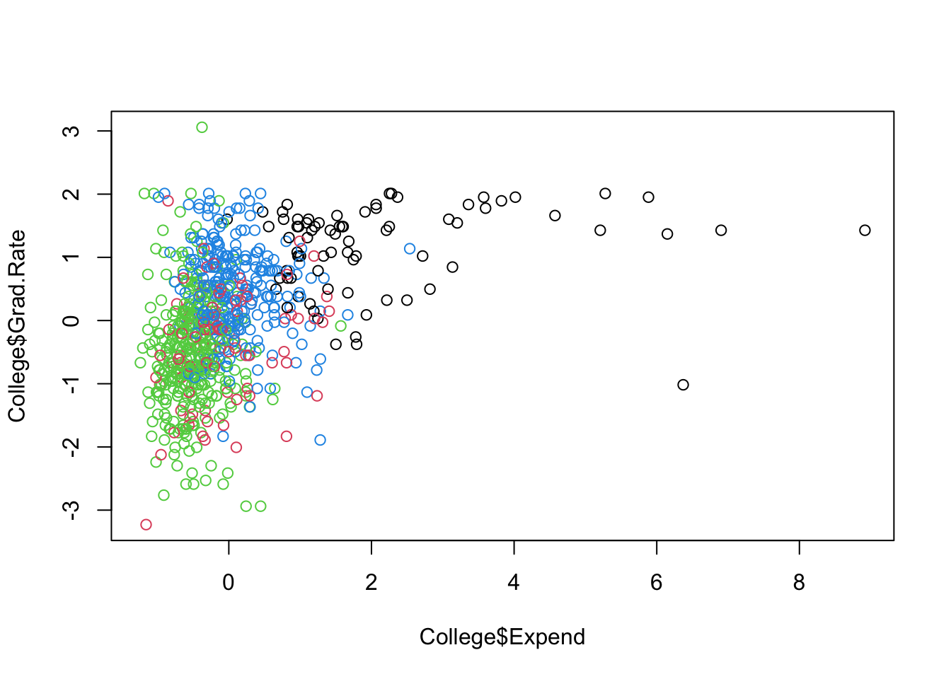
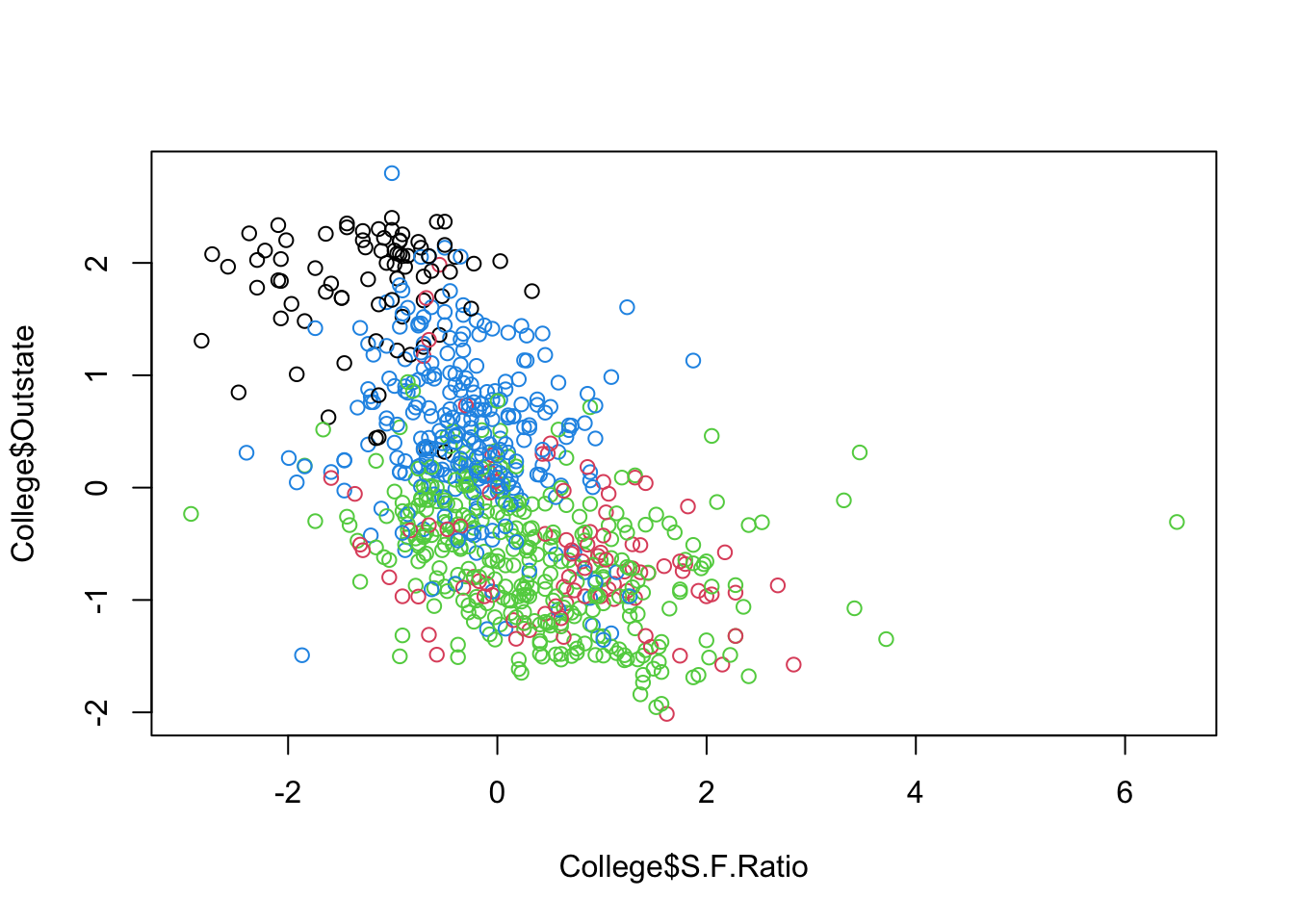
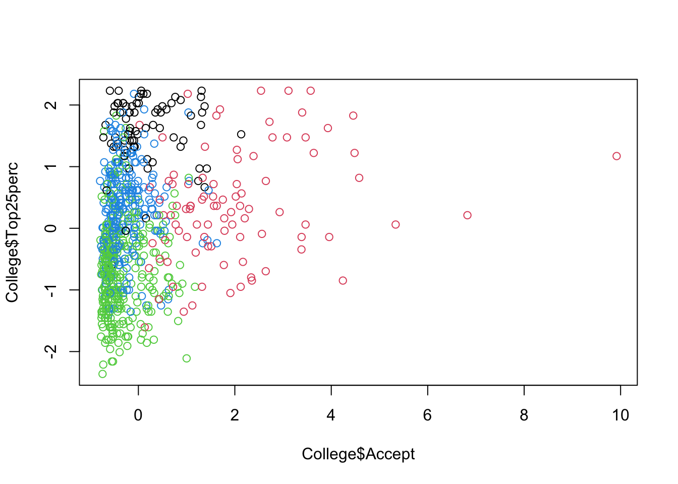
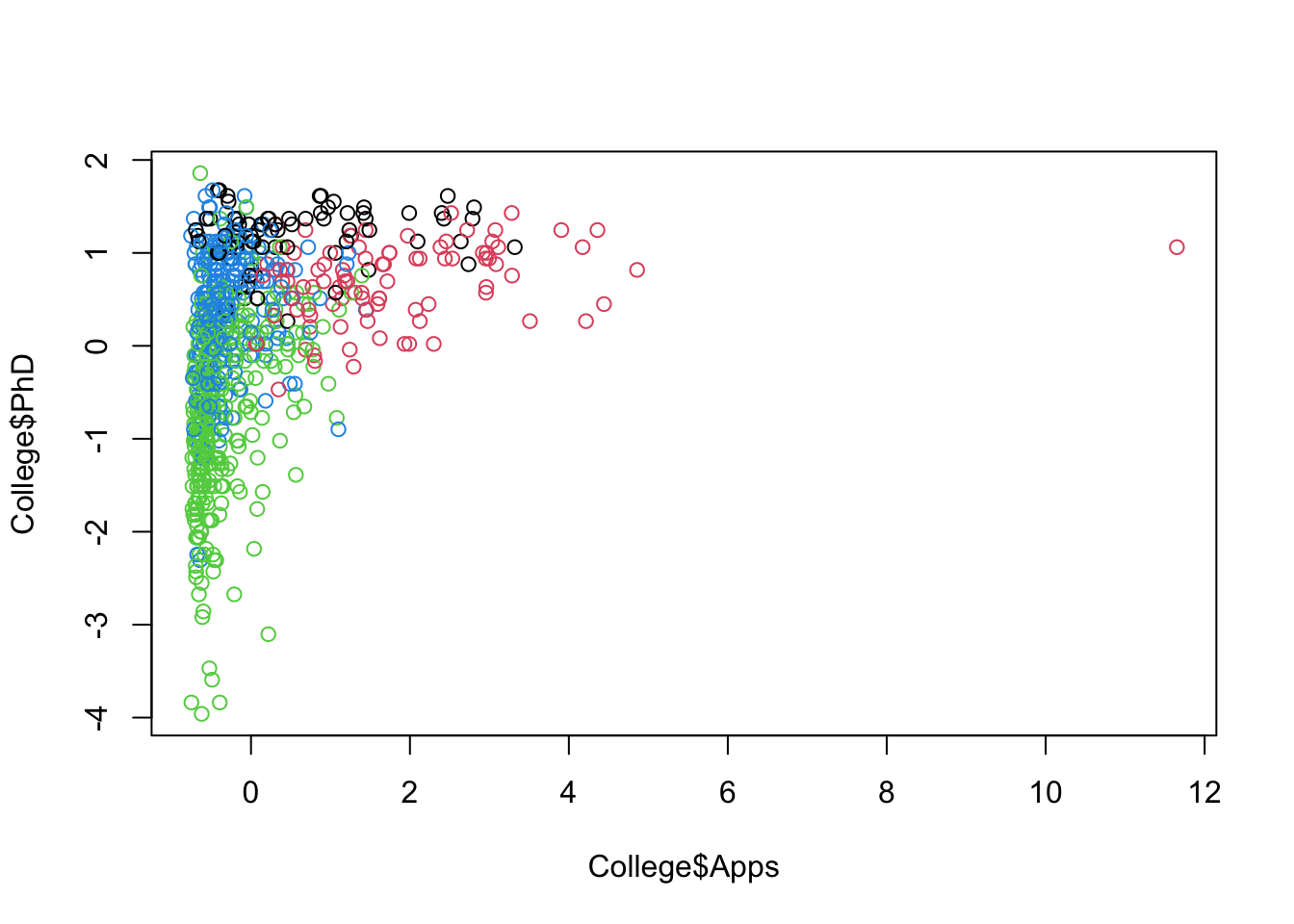
Let’s do some partial plots to try to understand the clusters.
Show code
Show code
ggplot(College, aes(Expend, Grad.Rate, color =  as.factor(KM4$cluster))) +
  geom_point(alpha = .8, size = .5) + labs(color = 'Cluster')
ggplot(College, aes(S.F.Ratio, Outstate, color = as.factor(KM4$cluster))) +
  geom_point(alpha = .8, size = .5) + labs(color = 'Cluster')
ggplot(College, aes(Accept, Top25perc, color = as.factor(KM4$cluster))) +
  geom_point(alpha = .8, size = .5) + labs(color = 'Cluster')
ggplot(College, aes(Apps, PhD, color = as.factor(KM4$cluster))) +
  geom_point(alpha = .8, size = .5) + labs(color = 'Cluster')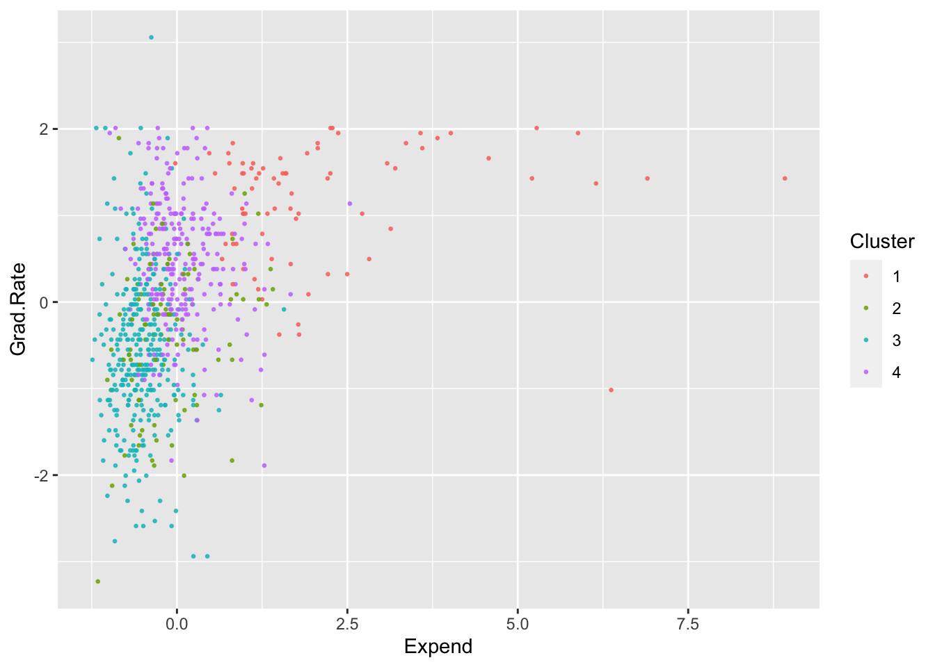
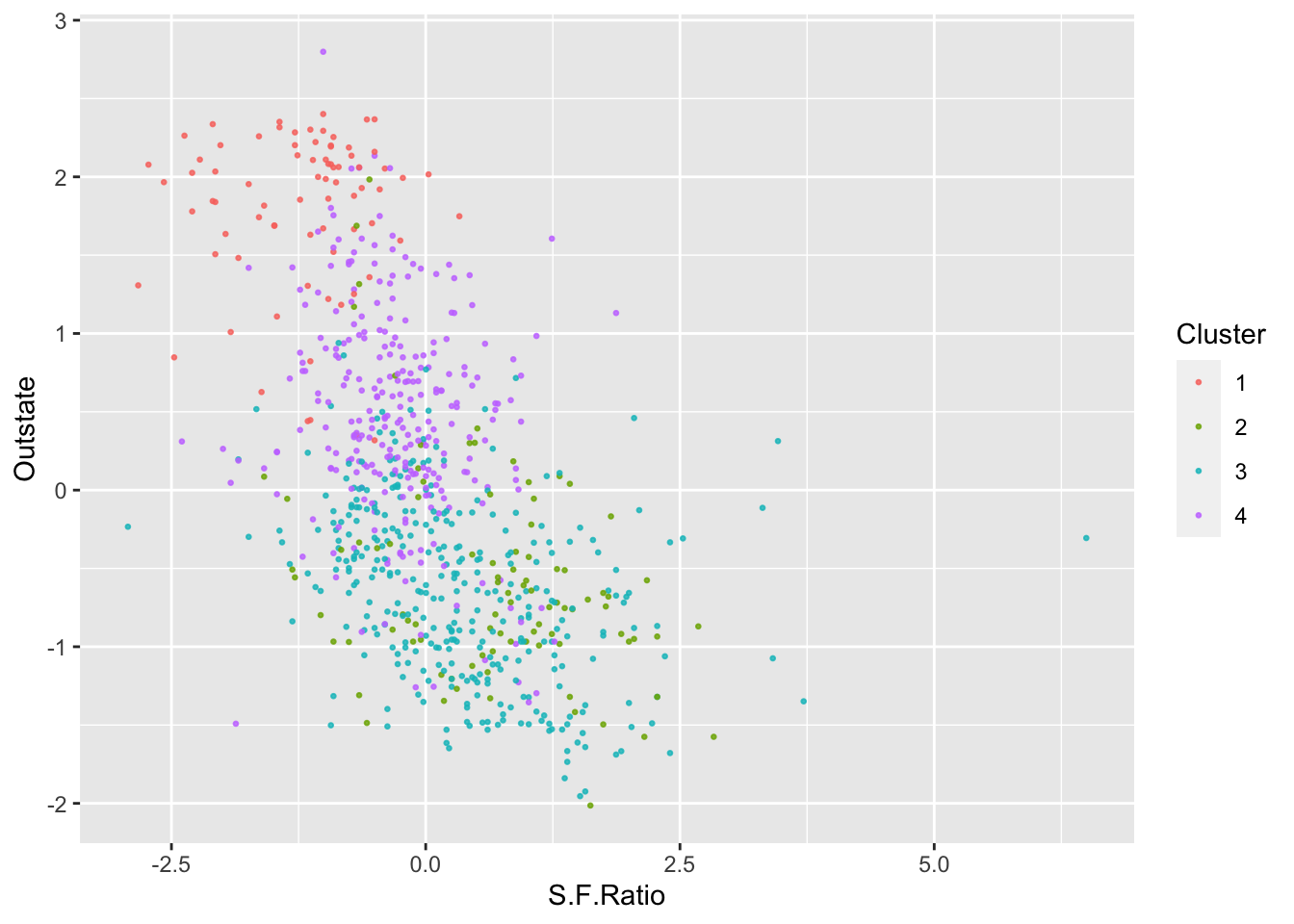
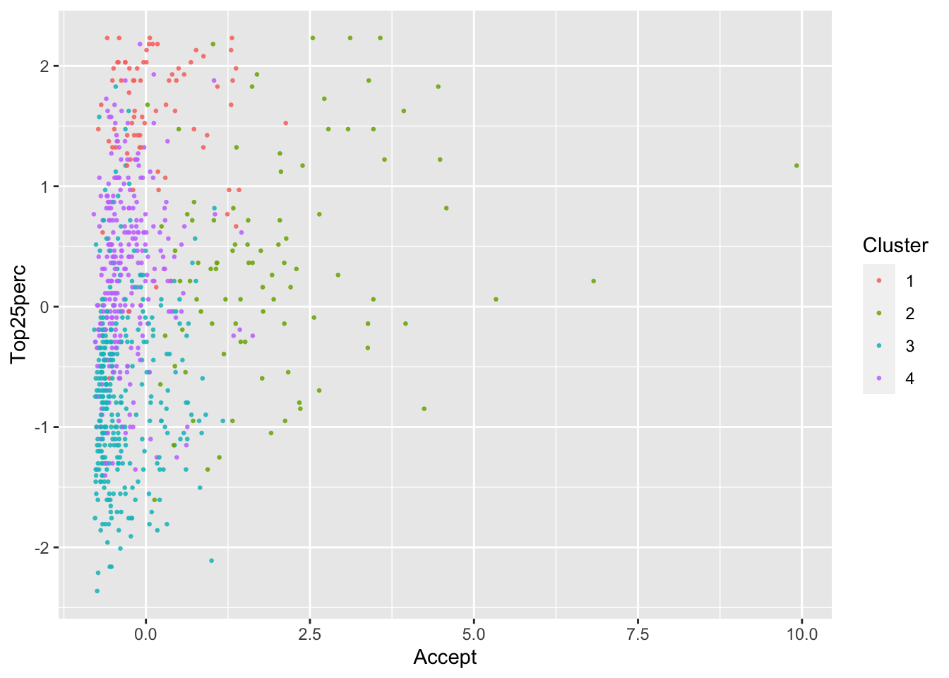
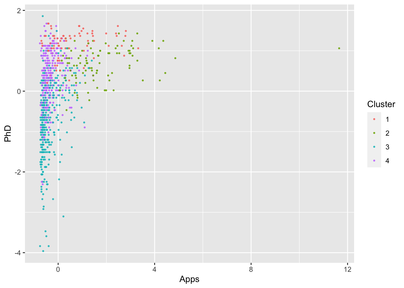
By looking at each cluster you can try to see how the clusters align with the various attributes of interest
10.5.3 Choosing K?
Some packages will create a plot of\(R^2\) vs \(K\) (see factoextra)
We will just create a short for-loop to iterate though various values of \(K\) and calculate the \(R^2\) and then plot.
k <- seq(2:700)
r2 <- vector("double", length = length(k))

for (i in seq_along(k)) {
  set.seed(123)
  tempk <- kmeans(X, k[i])
  r2[i] <- tempk$betweenss/tempk$totss
}
plot(k, r2)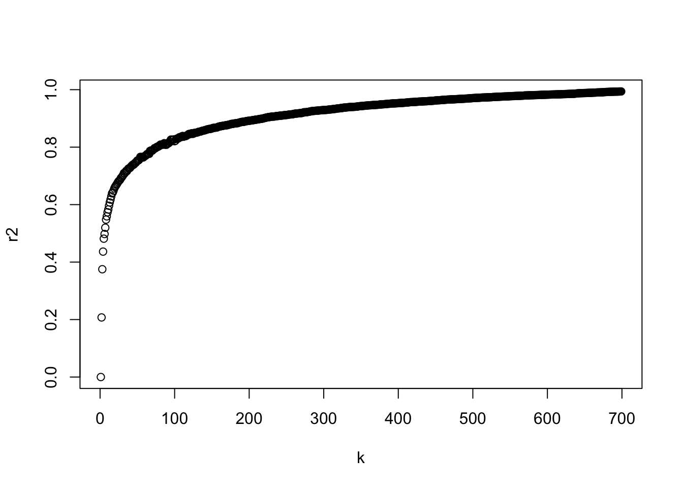
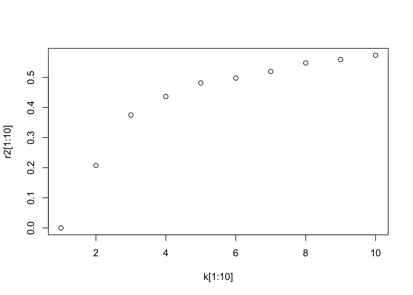
Since \(R^2\) is un-adjusted, we can see that increasing \(K\) will always increase \(R^2\).
Thus we look for a “knee” in the curve to find a reasonable solution.
Let’s look at just the first ten values and it seems \(k=4\) is not a bad choice.
10.5.4 Considerations for \(K\)-Means
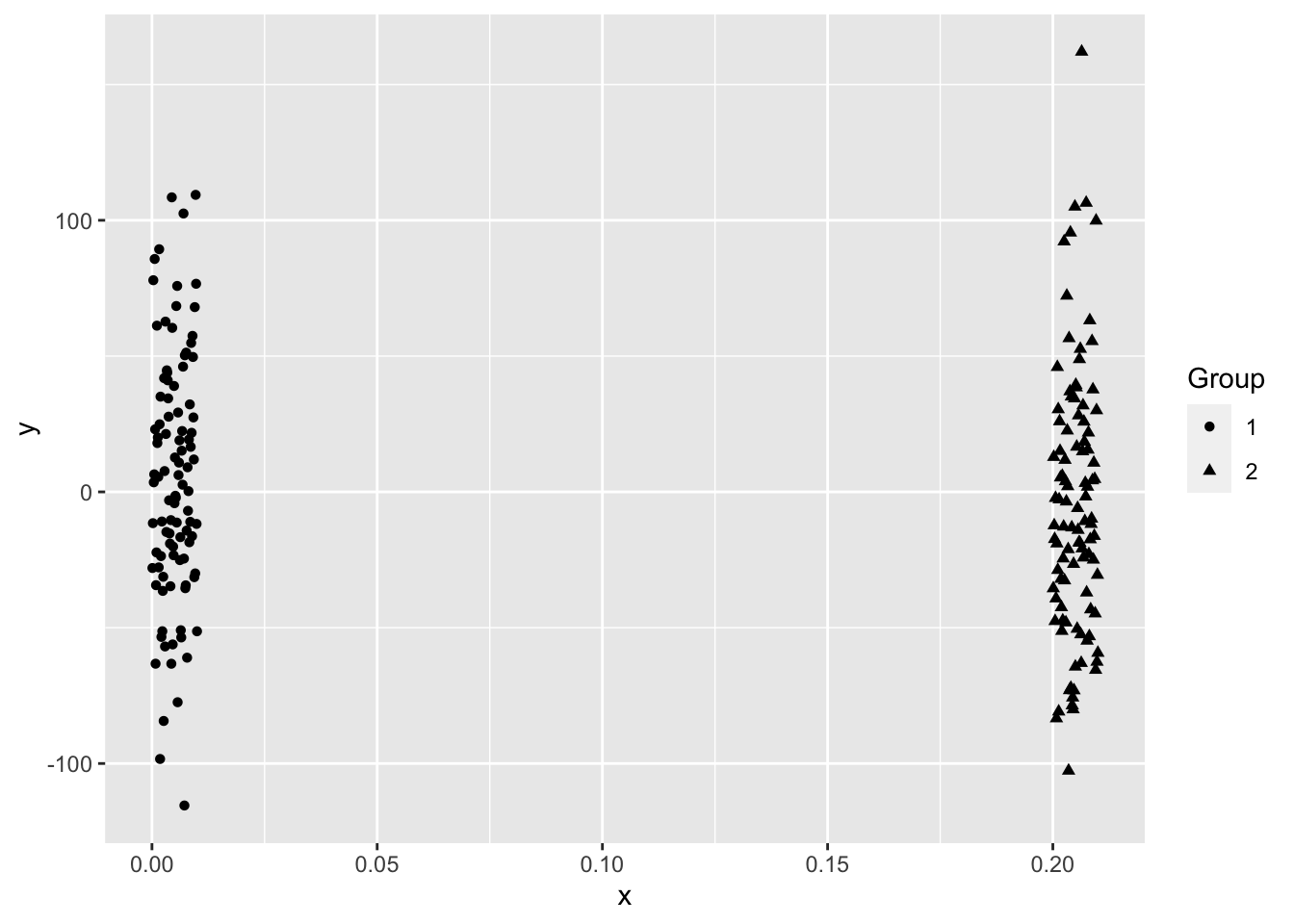
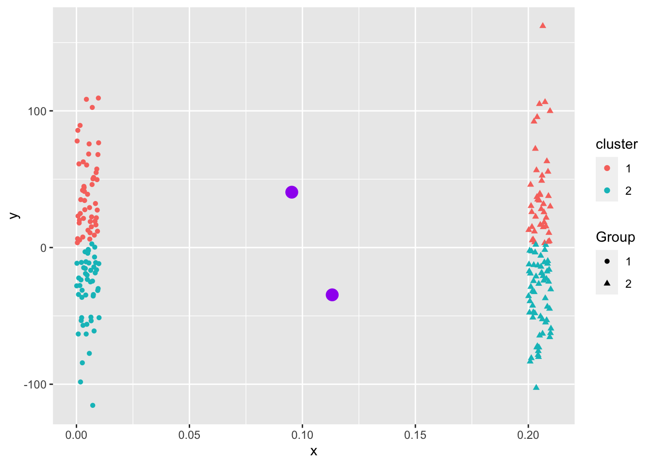
- Scaling matters. Not scaling can change the \(R^2\) by quite a bit as high magnitude variables will dominate the formation of the clusters.
- Scaling can help generate clusters with the same size.
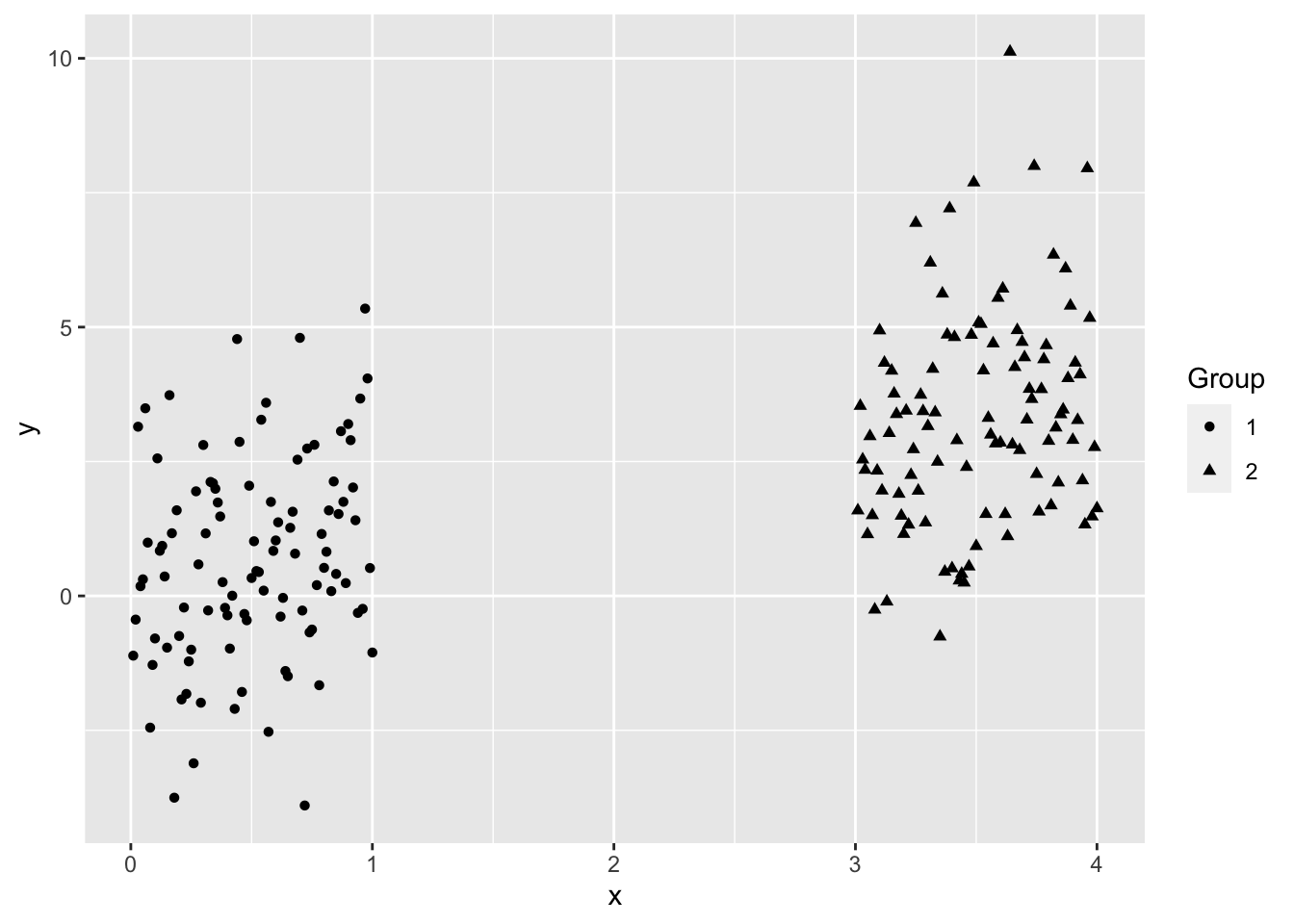
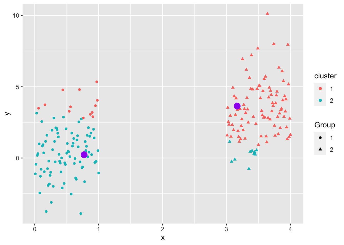
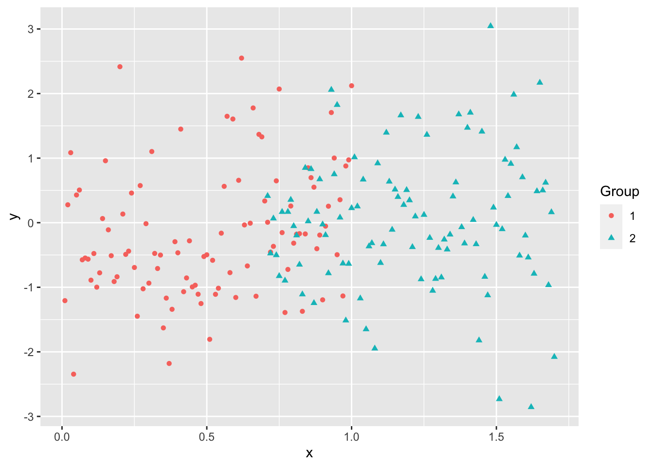
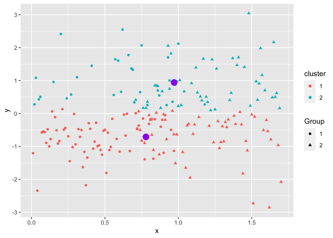
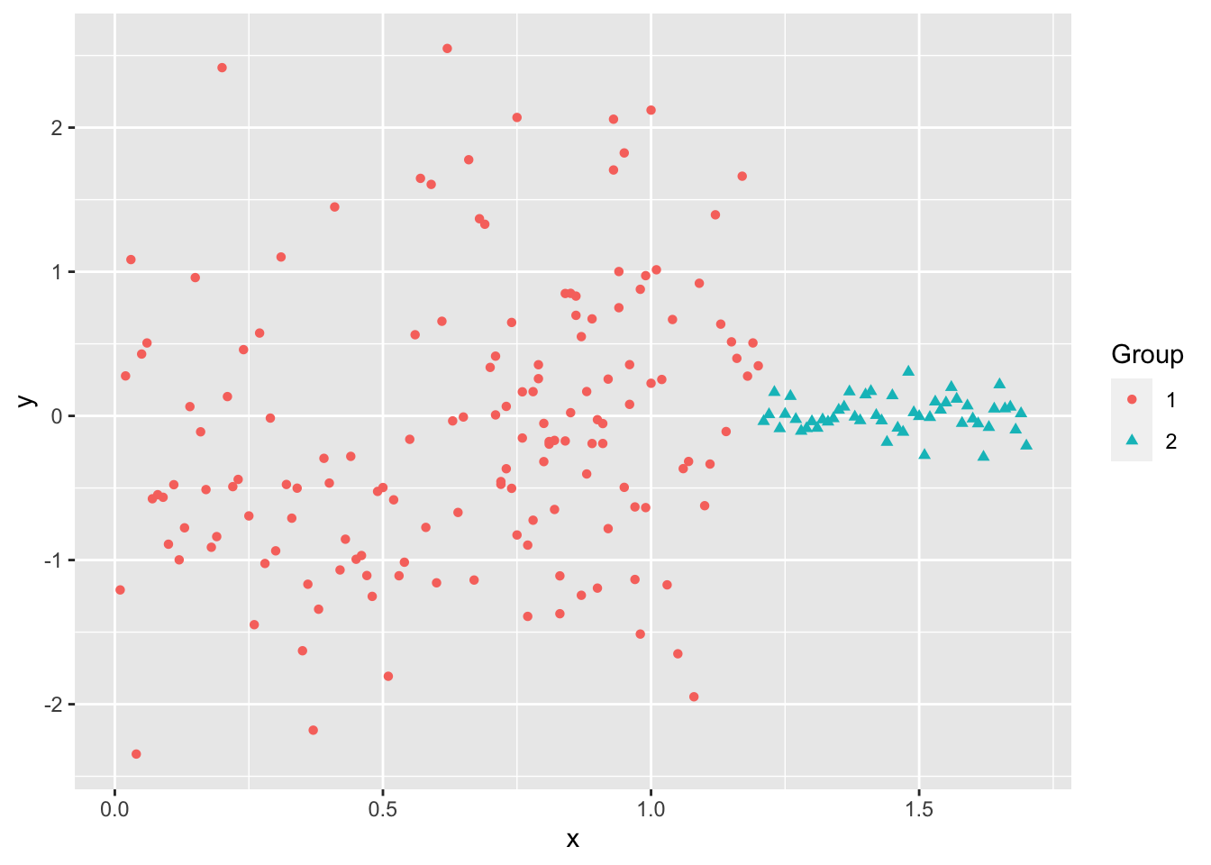
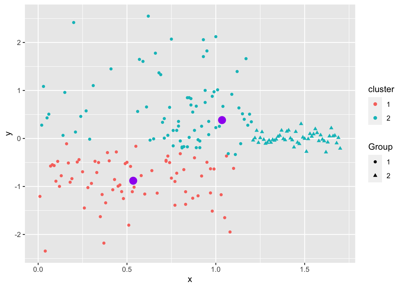
- Standard \(K\)-Means works best on data that can form clusters that are generally the same size, circular, and not overlapping.
Even when the data “looks nice”, the “local-optima” clusters can be off due to just enough noise.
Not circular, different magnitude.
Overlapping.
Not similar in size
\(K\)-means is a popular method for unsupervised learning to understand how observations might be clustered into meaningful groups.
Like all methods, use it with caution seasoned with some domain knowledge to assess interpretation and usefulness.
