2 Key Concepts in Statistical Machine Learning

ISLRv2 Chapters 1 and 2

Author

Affiliation

Richard Ressler

American University

Published

April 16, 2024

2.1 What is Statistical Machine Learning (SML)?

SML can be thought of as collection of statistical data analysis algorithms for analyzing and modeling data …

to better understand (“learn”) the relationships among the variables in the data, and,
to make estimates or predictions or classifications about new observations
in a repeatable manner.

SML algorithms can be:

Programmed on a computer (so can be repeated).
Evaluated quantitatively (using a computer) where prediction accuracy is our main measure of performance.
Tuned - optimized automatically. Every machine learning model can be adjusted and improved.

Important

Given a data set with $n$ observations of $X_{1}, \dots, X_{p}$ variables, SML algorithms estimate some fixed but unknown function $f (X)$ that

uses the information in the $X$ to make an inference about or predict the unknown value of $Y$ , and,
the predicted value $\hat{f} (X) = \hat{Y}$ is close to the true value of $Y$ ,
i.e., the error $\hat{Y} - Y = ϵ$ is small.

2.1.1 Two Main Goals or Uses of SML

Inference - learn about the data, fit models, test significance
Prediction - make statements about something that is not observed, is unknown, or uncertain.
Some combination of Inference or Prediction

Different goals are best met by different types of SML algorithms.

The ability to achieve a goal also depends upon the structure of the available data.

2.1.2 There are many Use Cases for SML across Domains

Two Examples:

Integrated Circuit Manufacturing - tiny devices with millions of transistors etc. Chips are produced in wafers with hundreds of chips on them that are cut into individual pieces for use.
- Companies test for good and bad chips and try to determine root cause of defects. Texas Instruments defined eight known root causes and a category for unknown.
- This is an example of predicting a root cause
Marketing
- A common SML method is clustering potential buyers of products.
- Different people look for different features of a product to spur their decision to buy.
- Marketeers group people into clusters so they can target them differently.
- They want people as similar as possible within clusters and as different as possible between clusters.
- Then you can analyze the characteristics of the clusters - average age, etc, …
- Once they learn the characteristics of a cluster they can target each cluster differently.

2.2 Perspectives on Statistical Machine Learning Methods/Models/Algorithms

SML methods/algorithms/modes can be described from multiple perspectives.

2.2.1 Supervised or Unsupervised Learning

These terms are about the structure of the available data: Is there a designated response variable?

Supervised Learning predicts or estimates an output based on one or more inputs.
- The data must have known values for at least one output variable, usually denoted by $Y$ , called the output variable (or the “response variable” or “dependent variable” where the values may be known as the “labels”).
- The data must also have values for one or more input variables, designated as $X_{1}, \dots, X_{p}$ , which may serve as “explanatory variables”, also known as “predictor variables”, “independent variables” or the “features.
- The data set may be “labeled data” where someone or something has identified the values of the designated response variable.
- The goal is to build a model that uses the values of the predictors to predict or estimate the unknown value of the associated response.
- We also want to understand which predictors are useful or not and by how much in our predictions.
- Methods include multiple forms of Regression.
Unsupervised Learning estimates the relationships among input variables when there is no designated output variable.
- We want to find the variables or “features” that help us differentiate or identify outcomes.
- The data has two or more input variables, $X_{1}, \dots, X_{p}$ but no output variables with values or labels.
- The data set is referred to as “unlabeled data” since no one has designated the values of the designated response variable, e.g., the text content of a tweet.
- Since there is no known output, it can be difficult to measure how well you are doing.
- Methods include classification, clustering, and principal components

Two other types of machine learning (not covered in this course) include:

Semi-supervised Learning combines a small amount of labeled data with a large amount of unlabeled data during training. The algorithms exploit one or more assumptions about the relationships betwen the labelled and unlabelled data to make choices.
Reinforcement Learning is a dynamic form of machine learning where the algorithm tries to determine an optimal set of decisions based on multiple choices over time.

2.2.2 Regression or Classification

Regression has a numerical/quantitative response or output.
Classification has a categorical output $Y$ that takes values from a discrete set of unordered categories.

2.2.3 Parametric or Non-Parametric

Parametric: We first assume some form of relationship for $f ()$ such that parameters of the relationship allow us to define a single fixed model from an assumed family of distributions.
- The form of $f$ may be linear or nonlinear.
- We use SML to estimate the parameters so as to make optimal predictions.
- This usually requires that the form of $\hat{f}$ is close to the true form of $f$ .
Non-Parametric: We don’t make any assumptions about the form of $f$ .
- This is more flexible and less restrictive

2.2.4 Flexible or Restrictive

A key concept in SML is choosing how flexible or non-flexible (restrictive) a model is by tuning the number of parameters (degrees of freedom) available for fitting the mode.

Flexible models have more parameters (or degrees of freedom) so they can more closely match the input data.
- Highly flexible models, with hundreds of parameters, can be complicated to interpret.
- They may be known as “blackbox” models - since we can’t explain what is happening inside the model to explain the prediction, e.g., why was someone turned down for a loan.
- Over-fitting the data occurs when a model is too flexible so it matches sample data so closely its predictions on new data have high variance.
Restrictive models have fewer parameters (or degrees of freedom).
- They can be easier to interpret but usually do not match the data as well.
- Under-fitting the data occurs when a model is too restrictive so it misses key features of the function $f$ and its predictions on new data have high bias.

2.2.5 Degrees of Freedom

The degrees of freedom (df or d.f.) is the number of dimensions of the space used to evaluate the variance.

2.2.5.1 Example of Sample Variance

When there are $X_{1}, \dots, X_{n}$ observations in a sample there are $n$ degrees of freedom to start.
To estimate the sample variance we use the following where the $X_{i} - \bar{X}$ are the residuals. $\begin{matrix} (2.1) & S^{2} = \frac{1}{(n - 1)} \sum_{i = 1}^{n} (X_{i} - \bar{X})^{2} \end{matrix}$
There is a constraint on the residuals. The sum of the set of residuals cannot have any possible value.
The one constraint is

$\sum (x_{i} - \bar{x}) = \sum X_{i} - n \bar{X} = \sum X_{i} - n \frac{\sum X_{i}}{n} = \sum X_{i} - \sum X_{i} = 0$

One constraint means the estimate of the variance has $n - 1$ degrees of freedom
This is why to get an unbiased estimate of $S^{2}$ is why we divide by $n - 1$ .

2.2.5.2 Example of a Regression Model

In a regression model with $p$ independent variables one can fit the model using “ordinary least squares”.
- That means one minimizes the sum of the squared errors $S S E = \sum ({\hat{y}}_{i} - y_{i})^{2}$
- The minimization is in terms of the parameters (for the intercept and the slopes) $β_{0}, β_{1}, \dots, β_{p}$ so there are $p + 1$ parameters
Regression requires solving $p + 1$ equations so there are $p + 1$ constraints.
- Thus the estimate of the variance, SSE, has $d f = n - number of constraints$ which means SSE has $d f = n - (p + 1)$

More degrees of freedom means a more flexible method or model.

Flexible methods or models follow the data more closely, e.g., adding a quadratic term allows a linear model to follow the data more closely than a single linear term.
A high-degree polynomial (e.g., a spline) can be quite curvy and be different on different parts of the data.
As an example, plot of Covid 19 cases in DC over time is highly non-linear so you probably should not use a linear model as splines might do better.

Show code

url <- c("https://raw.githubusercontent.com/CSSEGISandData/COVID-19/master/csse_covid_19_data/csse_covid_19_time_series/time_series_covid19_confirmed_US.csv")
readr::read_csv(url) |> 
  dplyr::filter(FIPS == 11001) |> 
  dplyr::select(tidyselect::contains("/")) |> 
  tidyr::pivot_longer(cols = tidyselect::contains("/"), names_to = "date", values_to = "cases", names_transform = lubridate::mdy) |> 
  dplyr::mutate(daily_cases = cases - dplyr::lag(cases)) |> 
  dplyr::filter(daily_cases != 0) ->
  covid_19_dc
rm(url)
covid_19_dc |> 
  ggplot2::ggplot(ggplot2::aes(date, daily_cases)) +
  ggplot2::geom_point() +
  ggplot2::geom_smooth(se = FALSE, method = lm, formula = y ~ x) +
  ggplot2::scale_y_log10() +
  ggplot2::labs(title = "Daily Covid Cases Reported in DC",
                subtitle = "log scale",
       caption = "COVID-19 Data Repository by the Center for Systems Science and Engineering (CSSE) at Johns Hopkins University") ->
  covid_19_dc_plot
covid_19_dc_plot

A point plot of the daily cases for Covid19 in DC showing the highly nonlinear nature of the data. A linear regression line does not fit the data well at all.

Is it good to be flexible?

Flexible methods have more parameters (d.f.) and can follow the sample data more closely
However, the higher the flexibility, the higher the variance so a too-flexible model may not predict very well.

Should you worry about the variance? Let’s look at our measure of performance.

2.3 Using Mean Squared Error (MSE) as a Measure of Performance for SML Algorithms

Prediction error is equivalent to prediction accuracy – How well can a model predict the unknown.

If we develop a method that has high variance it means there is a lot of noise in the predictions; change the data a little and the results or predictions can change quite a bit.

So, in Regression problems when we have a numerical response variable, performance will be measured by prediction mean squared error (MSE) defined as the expected value of the squared residuals:.

$\begin{matrix} (2.2) & M S E = E (\hat{y} - y)^{2} \end{matrix}$

$y$ is the actual value. This is typically from outside our data set as we don’t need to predict something we know from the data. We want to predict something we don’t know.
$\hat{y}$ is our prediction, which is computed from our observed data.

2.3.1 Let’s Look at the Elements of MSE

Let’s say we have a regression model where $y = f (x) + ϵ$ and

$f$ is some function of $x$ , it could be linear or non-linear.
$ϵ$ is our error term.

We estimate $f$ (denoted by $\hat{f}$ ) and if we plug in any vector $x$ we get the output $\hat{y}$ .

Let’s start with our definition of $M S E$ from Equation 2.2 and see if we can break it into pieces to better interpret what it means.

First add and subtract values into Equation 2.2 to get

$\begin{aligned} M S E & = E (\hat{y} - y)^{2} \\ = E {(\hat{f} (x) - E \hat{f} (x) + E \hat{f} (x) - E y + E y - y)}^{2} \end{aligned}$

Note: $\hat{f} (x) = \hat{y}$ , $E \hat{f} (x) = E \hat{y}$ and $E y = f (x)$ .

Now adding some parentheses we get

$\begin{matrix} (2.3) & M S E = E {((\hat{f} (x) - E \hat{f} (x)) + (E \hat{f} (x) - E (y)) + (E (y) - y))}^{2} \end{matrix}$

Each of the expectations is non-random – they are not random variables.
The right-side $y$ is something new - it’s not in our data set, and
The left-side predictor $\hat{y}$ is computed from the data.

Since the right side of Equation 2.3 is outside the data and the left side is in the data, it is reasonable to assume the left-side and right-side of Equation 2.3 are uncorrelated.

Note Equation 2.3 is in the form $(a + b + c)^{2}$ so it is straightforward to compute:

$\begin{matrix} (2.4) & M S E = E (\hat{f} (x) - E \hat{f} (x))^{2} + (E \hat{f} (x) - E y)^{2} + E (y - E y)^{2} + combination terms \end{matrix}$

Since the middle term of $(a + b + c)^{2}$ , ( $b$ ), is non-random, we don’t need to take another Expectation.
The combination terms include $a b$ or $b c$ where, since the $b$ terms are non-random the correlation is $0$ , and $a c$ which we already said are uncorrelated so the correlation is $0$ .

Removing the combination terms leaves three non-zero terms – the three elements or components of Mean Squared Error.

Let’s look at them starting on the right of Equation 2.4.

$\begin{matrix} (2.5) & M S E = E (\hat{f} (x) - E \hat{f} (x))^{2} + (E \hat{f} (x) - E y)^{2} + E (y - E y)^{2} \end{matrix}$

What is $E (y - E y)^{2}$ for any random variable? Consider if it were written $E (y - μ_{y})^{2}$ ?

It’s the variance of $Y$ our response variable.
What can we do about reducing this variance?
Nothing - it’s the randomness inherent in our response variable’s distribution.

Important

The randomness inherent in our response variable’s distribution* is called the Irreducible Error of MSE since we can’t reduce it.

The other two terms though are based on our data. Together they are called Reducible Error since we can effect them through increasing the size of our data set or using SML techniques and tuning.

If we look at the first term $E (\hat{f} (x) - E \hat{f} (x))^{2} = E (\hat{y} - E \hat{y})^{2}$ this is the variance of $\hat{y}$ our predicted value.

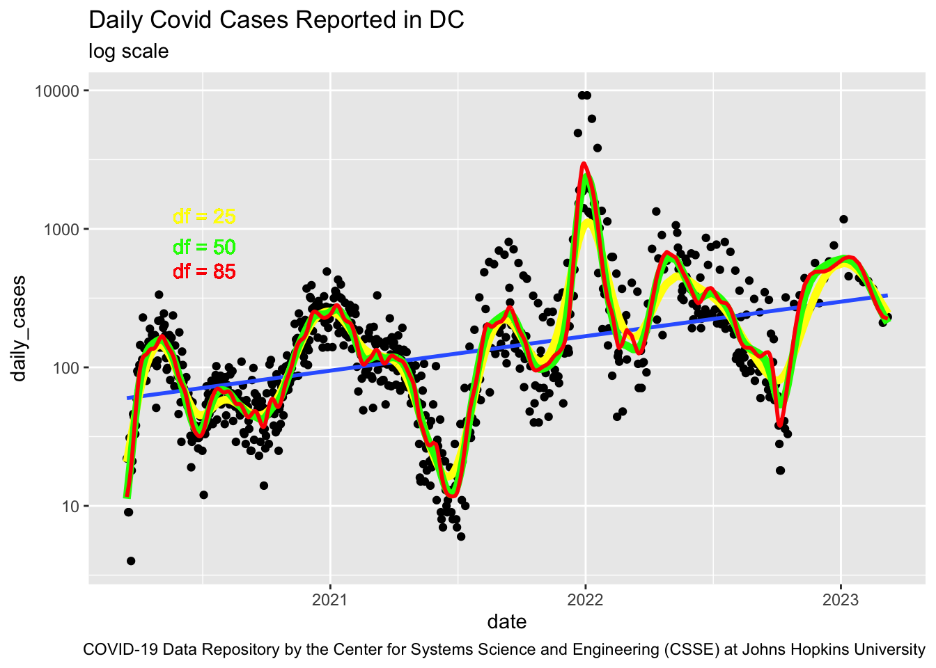
This is the variance that will increase with a flexible method with many degrees of freedom.
This is a term we want low.

Let’s look at the middle term $(E \hat{f} (x) - E y)^{2}$ which is also reducible.

Note the right side is $E y$ which is the unknown.
The difference between $E \hat{f} (x)$ and E $y$ is the bias of our prediction.
We want that to be small – to reduce the bias in our estimate.
If $(E \hat{f} (x) - E y) = 0$ then our estimated is called unbiased.
If the difference is not $0$ , then there is bias - our predictions are expected to be too high or too low.

This middle term in Equation 2.5 is the Squared Bias.

Alf Landon Example: Literary Digest sampled 10-million subscribers and predicted he would win the 1936 presidential election. Their subscribers tended to be wealthier, Republican, and leaning for Landon. Roosevelt won 46 of 48 states.

Important

MSE is our primary measure of performance for SML models
MSE has three components:
- Variance of $\hat{y}$ +
- Squared Bias +
- Irreducible Variance of $y$

Important

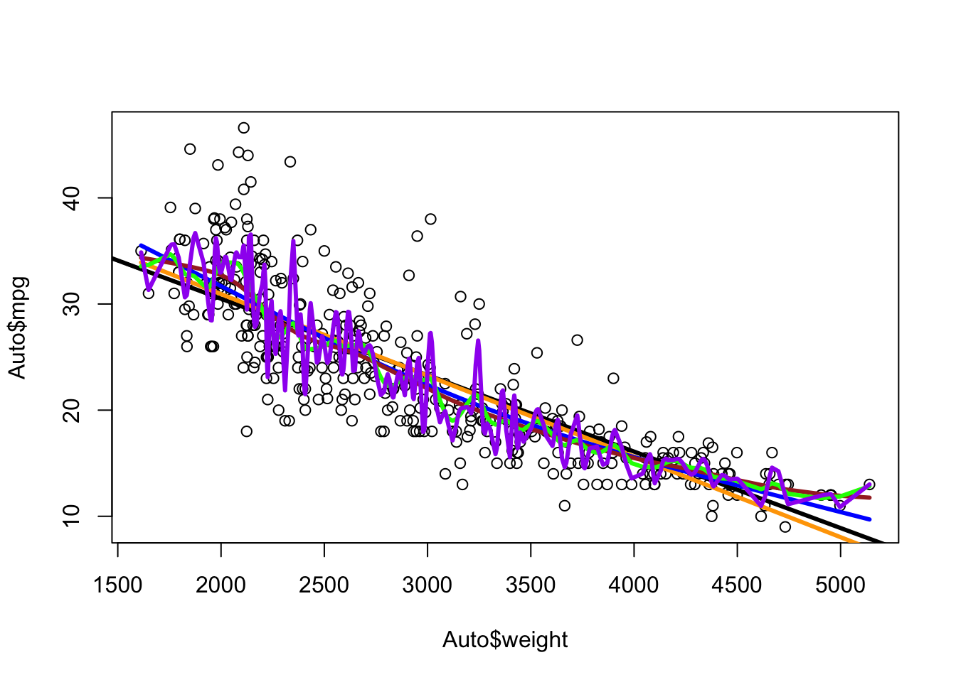
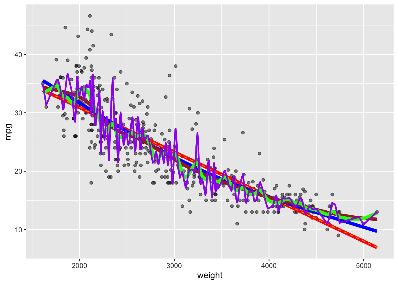
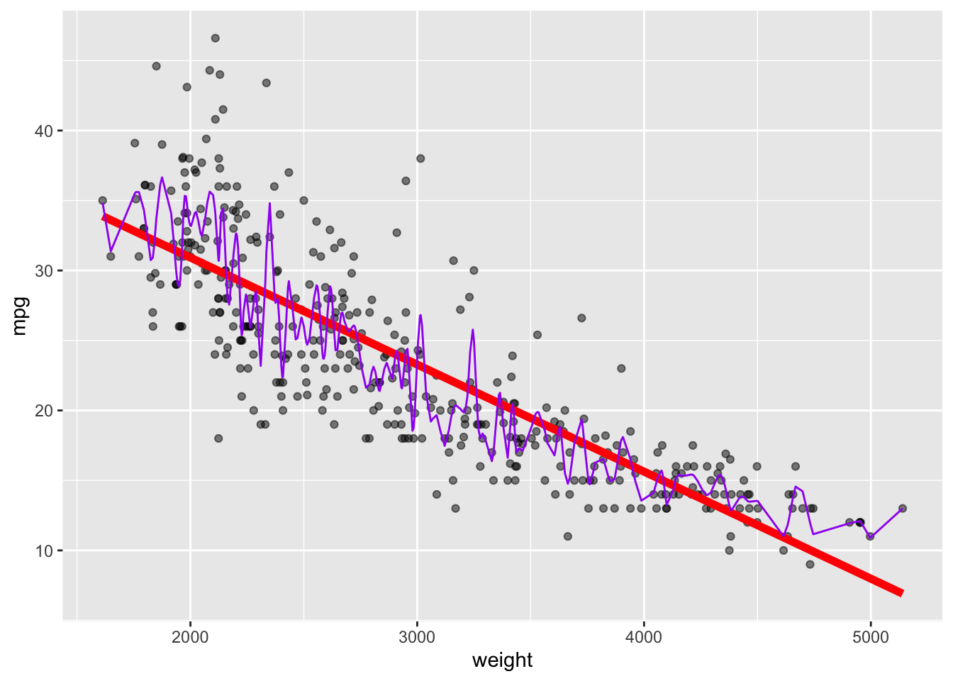
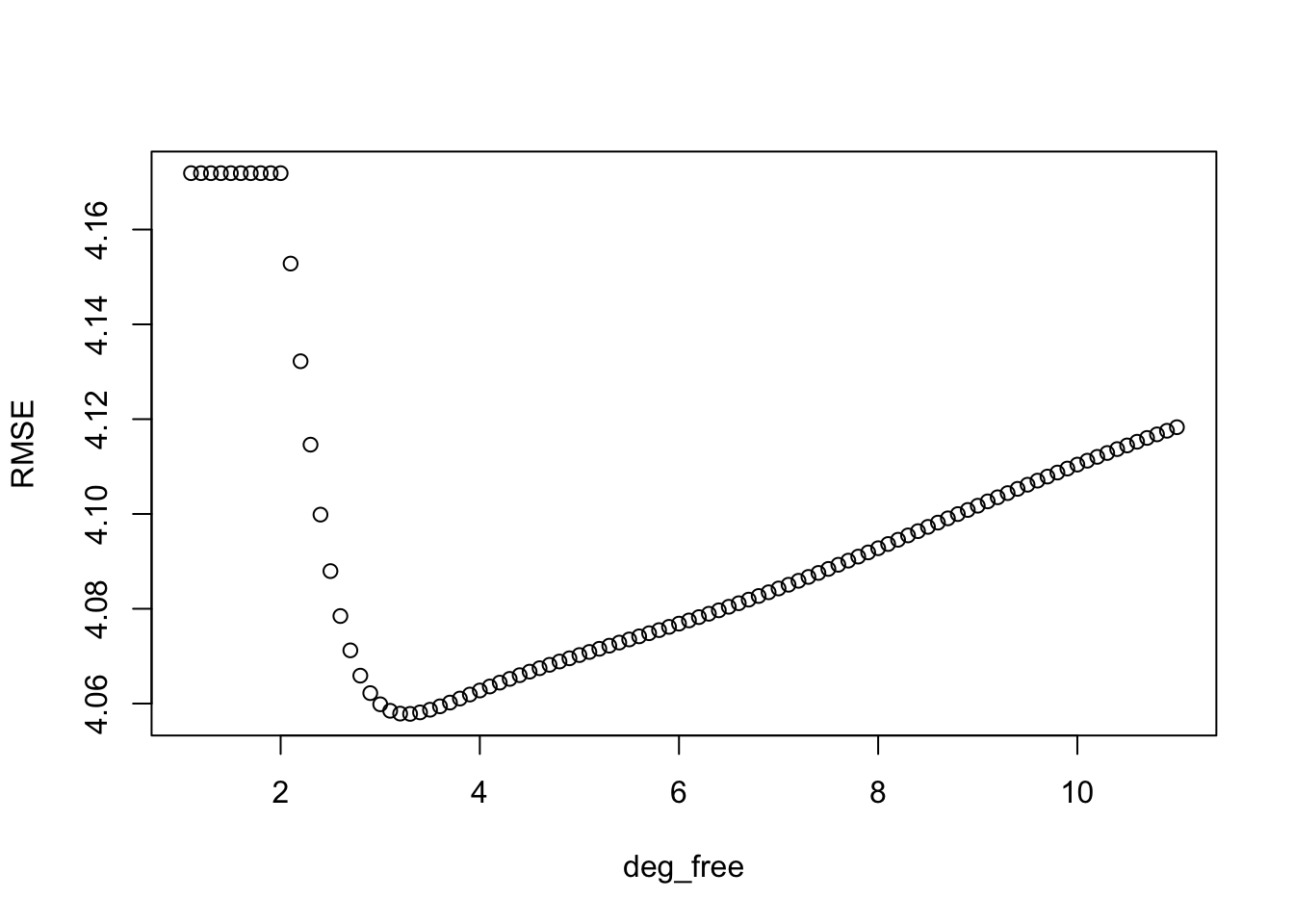
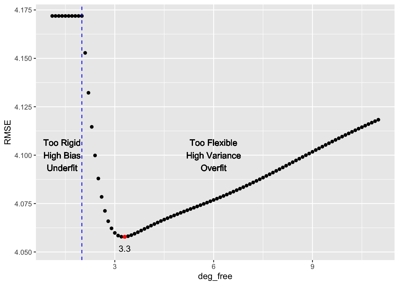
Flexible Methods have low bias as they can follow the data but can have high variance
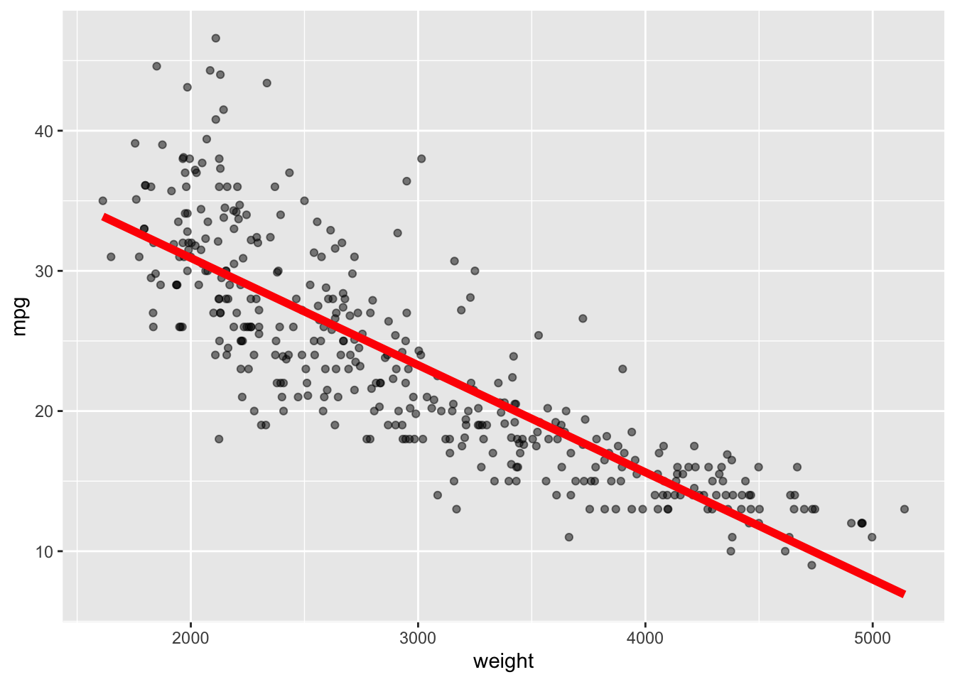
Restrictive Methods have low variance and high bias as they may not match all the data well.
This need to balance bias and variance in predictions is why SML is not just “plug and chug”– we have to think.

2.3.2 Estimating the MSE

We estimate the MSE for a regression problem by the sample MSE.

$\begin{matrix} (2.6) & M S E = E (\hat{y} - y)^{2} ⟹ \hat{M S E} = \frac{1}{n} \sum (y_{i} - {\hat{y}}_{i})^{2} \end{matrix}$

If we use the entire sample of size $n$ to estimate the MSE then

$\hat{M S E} = \frac{1}{n} \sum_{1}^{n} (y_{i} - {\hat{y}}_{i})^{2}$ is called the Training MSE also know as within the sample MSE since the MSE is estimated using the same data used to to fit the model.

What we really want is the error for our prediction - the Test MSE and it should be estimated from data outside the training sample.

Important

Prediction or Test MSE has to be estimated with data not used to train the model.

How do we do this? We split the data we have.

2.3.3 Splitting the Data

We split the sample data into sub-samples of Training Data and Test Data.

We use Training Data to fit the model – the learning part.
We use Test Data to evaluate the quality of the predictions with Prediction MSE.
The split should be a simple random sample, where every observation is equally likely to be chosen.

2.4 Example of Flexibility using R

2.4.1 Get the Data and Plot the Variables of Interest.

We will be using the Auto data set provided in the {ISLR2} package.

If you have not installed the package, please use your console to do so.

We are interested in the relationship between weight and mpg.

Base R
Tidyverse

Look at the names in the data set and plot.

Show code

library(ISLR2)
attach(Auto)
names(Auto)

[1] "mpg"          "cylinders"    "displacement" "horsepower"   "weight"      
[6] "acceleration" "year"         "origin"       "name"

Show code

plot(weight, mpg)

Show code

library(tidyverse)
library(ISLR2)
data("Auto")
ggplot(Auto, aes(x = weight, y = mpg)) +
  geom_point(alpha = .5) ->
base_plot
base_plot

It does not look quite linear.

Show code

reg = lm(mpg ~ weight, data = Auto) # calculate the parameters of the line
plot(Auto$weight, Auto$mpg)
abline(reg, col = "red", lwd = 3)

Show code

base_plot +
  geom_smooth(method = lm, se = FALSE, col = "red", linewidth  = 2) ->
base_plot
base_plot

Points seem to more below the line in the middle.

2.4.3 Calculate the Prediction MSE

To calculate the Prediction MSE, we will split the data in half into training and testing data sets.

To create a 50/50 split, we will get a random sample of size $n / 2$ where $n$ is the number of observations.
We can use that sample as a vector of indexes to subset the data set.
We will also set the seed for the pseudo-random number generator so our split of the observations is repeatable.

n <-  length(Auto$mpg)
n

[1] 392

set.seed(1234)
z <-  sample(n, n/2) # drawn from integers 1:n

Calculate the regression using the training subset of data selected by the indices in z.

reg <-  lm(mpg ~ weight, subset = z, data = Auto)

Use the testing data to generate the predictions for performance evaluation

Y <-  Auto$mpg[-z] # the True Y
Yhat <-  predict(reg, newdata = Auto[-z,]) # The predicted Y

Now you can calculate the prediction MSE using Equation 2.2.

Show code

MSE <- mean((Y - Yhat)^2)
MSE

[1] 17.25805

We don’t know yet if we can do better than 17.25805.

2.4.4 Check the Residuals

Linear Regression is quite a restrictive or inflexible method. It is probably not representing the data very well.

A quick plot of the residuals shows some curvature in them.

plot(reg)

2.4.5 Try a Spline Model

Let’s try a flexible spline model.

Spline models allow us to adjust the number of degrees of freedom or parameters in the model to provide more flexibility.
This makes df a hyper-parameter we can use later to tune our model.

Let’s start with df = 2. This is the same as simple linear regression with two parameters for intercept and slope.

Base R
Tidyverse

Calculate the spline with smooth.spline()

Show code

ss2 <-  smooth.spline(Auto$weight, Auto$mpg, df = 2)

Plot it.

Show code

plot(Auto$weight, Auto$mpg)
abline(reg, lwd = 3)
lines(ss2, col = "orange",lwd = 3)

Show code

library(ggformula) # the package for geom_spline
base_plot +
geom_spline(df = 2, color = "orange", lty = 2, linewidth = 2) ->
  base_plot2
base_plot2

Let’s increase the degrees of freedom which allows for more flexibility.

Use df = 3, then 10, then 40, and then 140.
This does not mean the spline is fitting only higher-order polynomials. It may decide to split into different polynomials for different parts of the data.

Base R
Tidyverse

Show code

plot(Auto$weight, Auto$mpg)
abline(reg, lwd = 3)
lines(ss2, col = "orange", lwd = 3)

ss3 <-  smooth.spline(Auto$weight, Auto$mpg, df = 3)
ss3 <-  smooth.spline(Auto$weight, Auto$mpg, df = 3)
lines(ss3, col = "blue", lwd = 3)

ss10 <-  smooth.spline(Auto$weight, Auto$mpg, df = 10)
lines(ss10, col = "brown", lwd = 3)

ss40 <-  smooth.spline(Auto$weight, Auto$mpg, df = 40)
lines(ss40, col = "green", lwd = 3)

ss140 <-  smooth.spline(Auto$weight, Auto$mpg, df = 140)
lines(ss140, col = "purple", lwd = 3)

Show code

base_plot +
  geom_spline(df = 2, color = "orange", lty = 2) +
  geom_spline(df = 3, color = "blue",  linewidth = 2) +
  geom_spline(df = 10, color = "brown", linewidth = 2) +
  geom_spline(df = 40, color = "green", linewidth = 2) +
  geom_spline(df = 140, color = "purple", linewidth = 1)

You can see as the degrees of freedom increase, the line is more flexible and matches the data better, but the model might be less accurate for prediction.

2.5 Using Test MSE to Explore Tuning a Model

We want to compare the prediction MSE across various versions of a regression model.

2.5.1 Splitting the Data

We start with splitting the data into Training and Test data sets.

Previously we split the data evenly in half - 50% Training and 50% Test.
What are the implications for this kind of split?
- How well will the model fit the data using only $n / 2$ points in the training data?
- Is there a “better split” than 50%?
- It appears we have another possible “hyper-parameter” for tuning our model.

Our formula for estimating the Test Data MSE for a regression problem is similar to Equation 2.6: ${\hat{M S E}}_{T e s t} = \frac{1}{n_{T e s t}} \sum_{i \in T e s t} (y_{i} - {\hat{y}}_{i})^{2}$

Note

If we want to calculate MSE for a Classification Problem, there are no $y_{i}$ so we have to use different methods.

We will be discussing later how to estimate the percentage of the time we predicted the correct classification, not the size of the residual.

We created multiple spline models where each had a different degrees of freedom.

The question is which was best? Can we optimize the model for the degrees of freedom that minimizes MSE.

As we saw in Equation 2.5, MSE has two elements that are reducible - the Bias and the Variance. We can’t do anything about the irreducible error.

Important

To minimize the MSE we have to find the balance between minimizing the variance of the estimates and the bias of the estimates.

This step in tuning the model is known as The Bias-Variance Trade-off.

2.5.2 Tuning an SML model

Tuning is optimization of a SML to minimize MSE – typically finding the optimal level of flexibility.

Let’s go back to the {ISLR} Auto data. Recall the plot with regression line of mpg vs weight.

Show code

base_plot

The plot suggests linear regression tends to underestimate mpg for the light and heavy cars and overestimate the mid-size cars.

When we add a highly flexible spline model (df = 100), it is much closer to the data but the accuracy of the predictions appear to be highly dependent upon the value of weight.

Show code

base_plot +
  geom_spline(df = 100, color = "purple")

Let’s try to tune our model.

Step one is create training and test data. Instead of splitting 50-50 let’s pick 200 cars for our training set - out of 392 observations.

Show code

set.seed(123)
z <-  sample(nrow(Auto),200)
training <-  Auto[z,]
test <-  Auto[-z,] # the complement of training

2.5.3 Fit a Regression Model

Let’s fit a regression model on the training data and check the summary.

Show code

reg <- lm(mpg ~ weight, data = training)
summary(reg)


Call:
lm(formula = mpg ~ weight, data = training)

Residuals:
    Min      1Q  Median      3Q     Max 
-9.0822 -2.7920 -0.4653  2.2020 16.4458 

Coefficients:
              Estimate Std. Error t value Pr(>|t|)    
(Intercept) 46.2373794  1.1255991   41.08   <2e-16 ***
weight      -0.0076223  0.0003641  -20.93   <2e-16 ***
---
Signif. codes:  0 '***' 0.001 '**' 0.01 '*' 0.05 '.' 0.1 ' ' 1

Residual standard error: 4.481 on 198 degrees of freedom
Multiple R-squared:  0.6888,    Adjusted R-squared:  0.6872 
F-statistic: 438.2 on 1 and 198 DF,  p-value: < 2.2e-16

Note the df is $198 = 200 - 2 parameters$ .

We will use this model to make our predictions. We can predict for the entire data set and then select the -Z indexed values to calculate $M S E_{t e s t}$

Yhat <-  predict(reg, newdata = Auto)
MSE_test <-  mean((Yhat[-z] - Auto$mpg[-z])^2)
MSE_test

[1] 17.44414

What’s the unit of measure for MSE_test? – It’s miles-squared per gallons-squared – a bit hard to interpret.

What can we do? – take the square root to give us the Root Mean Squared Error (RSME).

RMSE_reg <- sqrt(MSE_test)
RMSE_reg

[1] 4.176619

So the liner regression model is predicting within $\pm$ 4.1766186

We could add more more variables from the data set, besides weight, which would make the model more flexible. How do we know if it makes it too flexible?

2.5.4 Fit a more flexible spline model instead

Show code

ss <-  smooth.spline(Auto$weight[z], Auto$mpg[z], df = 100)

Make the predictions. Note predict() returns a list of x and y. All we want is the y element.

Yhat <- predict(ss, Auto$weight[-z])
str(Yhat)

List of 2
 $ x: int [1:192] 3504 3693 3436 4341 4312 3609 2372 2774 2587 2130 ...
 $ y: num [1:192] 18.3 22.2 16.1 15.4 13.9 ...

Yhat <- predict(ss, Auto$weight[-z])$y

Get the RSME and compare to RMSE_Reg

RMSE_ss <- sqrt(mean((Yhat - Auto$mpg[-z])^2))
RMSE_ss

[1] 6.205467

RMSE_reg

[1] 4.176619

Note that building splines actually allows for fractional degrees of freedom as long as $d f \geq 1$ . Hard to imagine in our minds, but mathematically fine.

Let’s use this to see if we can find an optimal value for our RMSE.

2.5.5 Fitting Many Models

Let’s fit 100 spline models with different degrees of freedom and plot how the RMSE changes with degrees of freedom.

Base R
Tidyverse

Show code

set.seed(123)
z <-  sample(nrow(Auto),200)
deg_free <- seq(1.1, 11, .1)
RMSE = rep(0, length(deg_free))
for (k in seq_along(RMSE)) {
  ss <-  smooth.spline(x = Auto$weight[z], y = Auto$mpg[z], df = deg_free[k])
  Yhat <-  predict(ss, x =  Auto$weight[-z])$y
  RMSE[k] <- sqrt(mean((Yhat - Auto$mpg[-z])^2))
}
plot(deg_free, RMSE)

Show code

set.seed(123)
z <-  sample(nrow(Auto),200)
deg_free <- seq(1.1, 11, .1)
calc_rmse_spline <- function(x, y, index, df){
  ss <-  smooth.spline(x = x[index], y = y[index], df = df)
  Yhat <-  predict(ss, x = x[-index])$y
  RMSE <- sqrt(mean((Yhat - y[-index])^2))
}

RMSE <- map_dbl(deg_free, ~ calc_rmse_spline(Auto$weight, Auto$mpg, z, .))

Show code

ggplot(bind_cols(deg_free = deg_free, RMSE = RMSE), aes(deg_free, RMSE)) +
  geom_point() +
  geom_point(aes(x = deg_free[(RMSE == min(RMSE))], y = min(RMSE)), color = "red") + 
  geom_text(aes(x = deg_free[(RMSE == min(RMSE))], y = min(RMSE)), label = (deg_free[(RMSE == min(RMSE))]), nudge_y = -.006,check_overlap = TRUE) + 
  geom_vline(xintercept = 2, color = "blue", lty = 2) +
  geom_text(aes(x = 1.4, y = 4.1), label = "Too Rigid\nHigh Bias\nUnderfit") +
  geom_text(aes(x = 6, y = 4.1), label = "Too Flexible\nHigh Variance\nOverfit")

What happens if we change the seed for selecting our sample? What happens if we change our sample size?

Try the shiny app for Exploring Splines with the ISLR2 Auto Data.

Important

Selecting the hyper-parameter(s) to create a model that optimizes the bias variance trade-off is a typical challenge in Data Science.

2.5.6 DC Covid Data Example Continued

Recall this plot?

Show code

covid_19_dc_plot

How many splines are optimal??

Show code

url <- c("https://raw.githubusercontent.com/CSSEGISandData/COVID-19/master/csse_covid_19_data/csse_covid_19_time_series/time_series_covid19_confirmed_US.csv")
readr::read_csv(url) |> 
  dplyr::filter(FIPS == 11001) |> 
  dplyr::select(tidyselect::contains("/")) |> 
  tidyr::pivot_longer(cols = tidyselect::contains("/"), names_to = "date", values_to = "cases", names_transform = lubridate::mdy) |> 
  dplyr::mutate(daily_cases = cases - dplyr::lag(cases)) |> 
  dplyr::filter(daily_cases != 0) ->
  covid_19_dc
rm(url)

set.seed(1234)
z <-  sample(nrow(covid_19_dc),floor(nrow(covid_19_dc)*.6))
deg_free <- seq(2, 100, 1)

RMSE <- map_dbl(deg_free, ~ calc_rmse_spline(as.integer(covid_19_dc$date), covid_19_dc$daily_cases, z, .))

Show code

ggplot(bind_cols(deg_free = deg_free, RMSE = RMSE), aes(deg_free, RMSE)) +
  geom_point() +
  geom_point(aes(x = deg_free[(RMSE == min(RMSE))], y = min(RMSE)),
             color = "red") +
  geom_text(aes(x = deg_free[(RMSE == min(RMSE))], y = min(RMSE)),
            label = (deg_free[(RMSE == min(RMSE))]), nudge_y = -6,
            check_overlap = TRUE) +
  geom_vline(xintercept = 2, color = "blue", lty = 2)

Show code

covid_19_dc_plot +
  geom_spline(df = 25, color = "yellow", linewidth = 2) +
  geom_spline(df = 50, color = "green", linewidth = 2) +
  geom_spline(df = 85, color = "red", linewidth = 1) +
  geom_text(aes(x = lubridate::mdy("07/05/2020"), y = 1250), label = "df = 25", color = "yellow") +
  geom_text(aes(x = lubridate::mdy("07/05/2020"), y = 750), label = "df = 50", color = "green") +
  geom_text(aes(x = lubridate::mdy("07/05/2020"), y = 500), label = "df = 85", color = "red")

What does this suggest to you?

2.6 Classification and MSE

Concepts such as bias-variance trade-off and optimizing flexibility to minimize MSE are applicable in classification models, but the formulas are different.

Suppose we have a data set of $n$ observations of $p$ variables $x_{1}, \dots, x_{p}$ but the output $y_{i}$ is categorical, not quantitative.

We still want to estimate $f ()$ based on the information in the set of $x_{i}$ .

2.6.1 Training Error Rate

To calculate the accuracy of our estimate $f ()$ , $\hat{f} ()$ , we can use the training error rate – the proportion of observations that are mis-classified by our $\hat{f} ()$ applied to the training data.

$\begin{matrix} (2.7) & Training Error Rate = \frac{1}{n} \sum_{i = 1}^{n} I ({\hat{y}}_{i} \neq y_{i}) \end{matrix}$

In Equation 2.7, ${\hat{y}}_{i}$ is the predicted value for $\hat{f} (x_{i})$ and $I ({\hat{y}}_{i} \neq y_{i})$ is an Indicator variable such that

$I = {\begin{cases} 0 & {\hat{y}}_{i} = y_{i}) & Correct Classification \\ 1 & {\hat{y}}_{i} \neq y_{i}) & Incorrect Classification \end{cases}$

So, Equation 2.7 is training error rate as it is calculating the fraction of incorrect classifications based on the training data.

2.6.2 Test Error Rate

If we apply our $\hat{f} (X)$ to test data, new observations not used in training the classifier, then we get the test terror rate.

$\begin{matrix} (2.8) & Test Error Rate = Average (I ({\hat{y}}_{i} \neq y_{i})) \end{matrix}$

where ${\hat{y}}_{i}$ is the predicted category label based on applying $\hat{f} (x)$ to test predictors $x_{i}$ .

We want to optimize our classifier by minimizing the test error rate in Equation 2.8.

We will discuss classification methods in much greater detail, but the same concepts apply.

Important

Optimizing SML models depends on solving the bias-variance trade off.