8 Tree Methods
8.1 Why Trees
Trees are popular because they are intuitive and easy to understand.
- Certainly easier than principal components with its uninterpretable linear combinations.
- However, this can come at a cost of lower performance.
Let’s try an example of making a decision - Do we want to buy a given house?
We start by asking a series of yes-no questions.
- Is it affordable - yes or no?
- For each response we make a decision: Buy if Yes, or if No, ask another question.
- We ask as many questions as we need to make a final decision.
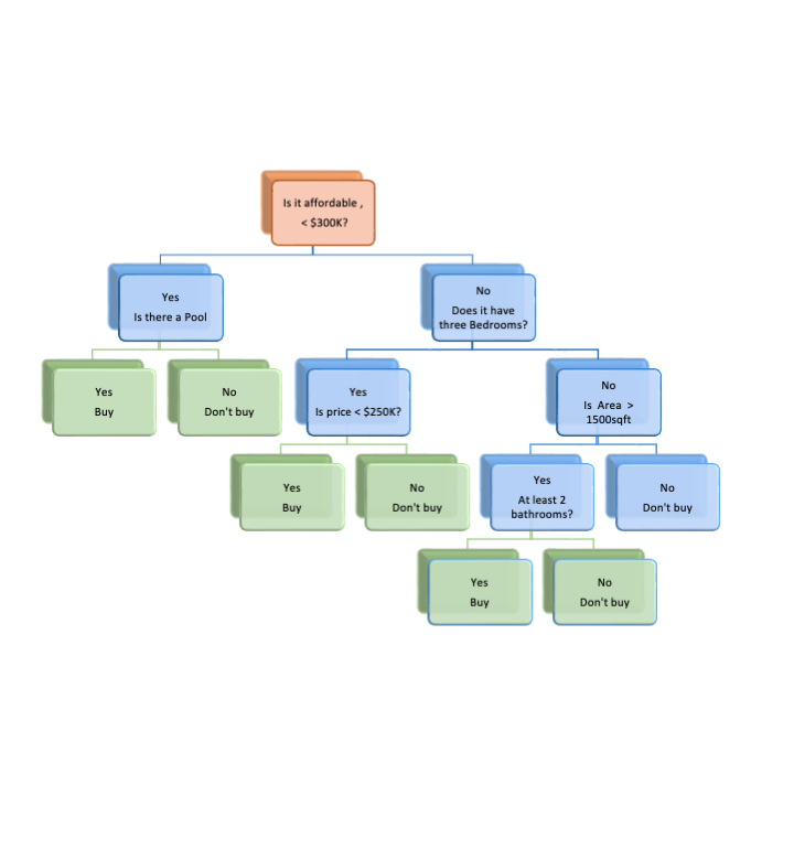
The (upside-down) tree in Figure 8.1 represents the way many people think they make decisions.
- They examine alternatives one by one and make a “rational” choice.
8.2 The Structure of Trees
- A tree has a root.
- It splits into branches.
- Each split is a node.
- A node with no splits (lowest on its branch), where we make a final decision, is called a terminal node or a leaf.
8.3 Types of Trees
There are Classification Trees and Regression Trees.
Classification Trees predict a categorical response.
- Buy the house or not?
- They are not limited to just binary responses.
Regression Trees predict a quantitative response.
- How much is a fair price for the house?
- At every internal node, it decides how to split for the best prediction.
People use analogies such as “growing” and “pruning” to describe creating the splits and then removing splits to trim the size of the tree (to avoid overfitting).
At each internal node you choose two things
- A variable
- A threshold for the variable to provide the best prediction (the decision).
Every terminal node \(m\) will make one prediction, a \(\hat{Y}_m\) for all the sampling units (\(X_j\)) remaining in the \(m\)th node.
For regression trees, \(\hat{y}_m\) is the sample mean of all the responses that fit in the \(m\)th node.
For classification trees, use “majority rules” (like KNN) so \(\hat{y}_m\) is the most frequent response of all the responses that fit in the \(m\)th node. It’s the mode of the responses remaining in the node.
8.4 Trees in R with {tree}
8.4.1 Fitting and Plotting Trees
The R {tree} package has functions for fitting and plotting trees.
Let’s start with fitting the HOMES_SALES data.
Download the HOME_SALES data from https://raw.githubusercontent.com/rressler/data_raw_courses/main/HOME_SALES.csv
Show code
Rows: 522
Columns: 13
$ ID <dbl> 1, 2, 3, 4, 5, 6, 7, 8, 9, 10, 11, 12, 13, 14, 15, 16,…
$ SALES_PRICE <dbl> 360000, 340000, 250000, 205500, 275500, 248000, 229900…
$ FINISHED_AREA <dbl> 3032, 2058, 1780, 1638, 2196, 1966, 2216, 1597, 1622, …
$ BEDROOMS <dbl> 4, 4, 4, 4, 4, 4, 3, 2, 3, 3, 7, 3, 5, 5, 3, 5, 2, 3, …
$ BATHROOMS <dbl> 4, 2, 3, 2, 3, 3, 2, 1, 2, 3, 5, 4, 4, 4, 3, 5, 2, 4, …
$ GARAGE_SIZE <dbl> 2, 2, 2, 2, 2, 5, 2, 1, 2, 1, 2, 3, 3, 2, 2, 2, 2, 2, …
$ YEAR_BUILT <dbl> 1972, 1976, 1980, 1963, 1968, 1972, 1972, 1955, 1975, …
$ STYLE <dbl> 1, 1, 1, 1, 7, 1, 7, 1, 1, 1, 7, 1, 7, 5, 1, 6, 1, 7, …
$ LOT_SIZE <dbl> 22221, 22912, 21345, 17342, 21786, 18902, 18639, 22112…
$ AIR_CONDITIONER <chr> "YES", "YES", "YES", "YES", "YES", "YES", "YES", "YES"…
$ POOL <chr> "NO", "NO", "NO", "NO", "NO", "YES", "NO", "NO", "NO",…
$ QUALITY <chr> "MEDIUM", "MEDIUM", "MEDIUM", "MEDIUM", "MEDIUM", "MED…
$ HIGHWAY <chr> "NO", "NO", "NO", "NO", "NO", "NO", "NO", "NO", "NO", …Recall that QUALITY has three levels.
Let’s predict house quality as a function of the other variables.
Let’s build/fit a classification tree and plot it.
- Note: convert
QUALITYto a factor. -
plot()callstree::plot.tree().
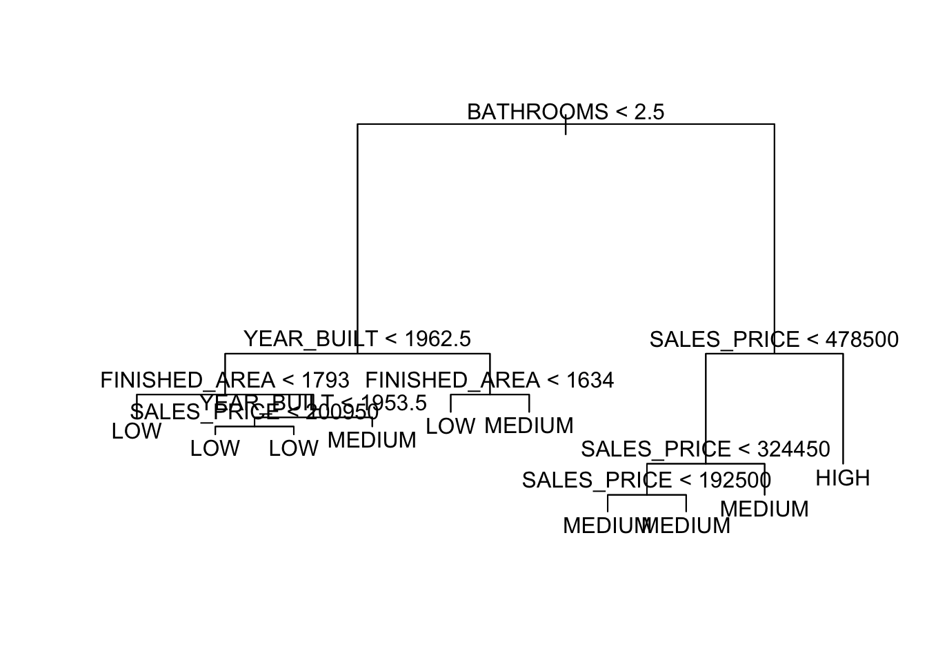
We get a plot, but it’s hard to interpret as is.
Let’s add some text
-
text()callstext.tree()
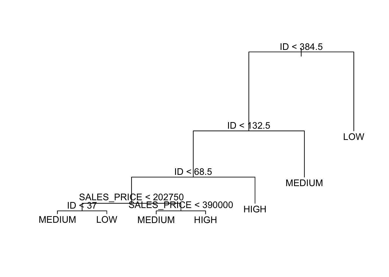
What do you think it means that ID seems so important?
- This data set happens to have high quality houses lower in the the order.
- That suggests the tree would do poorly predicting new data that happened to be in a different order or even have a different number of rows of each kind of quality.
Let’s refit without ID.
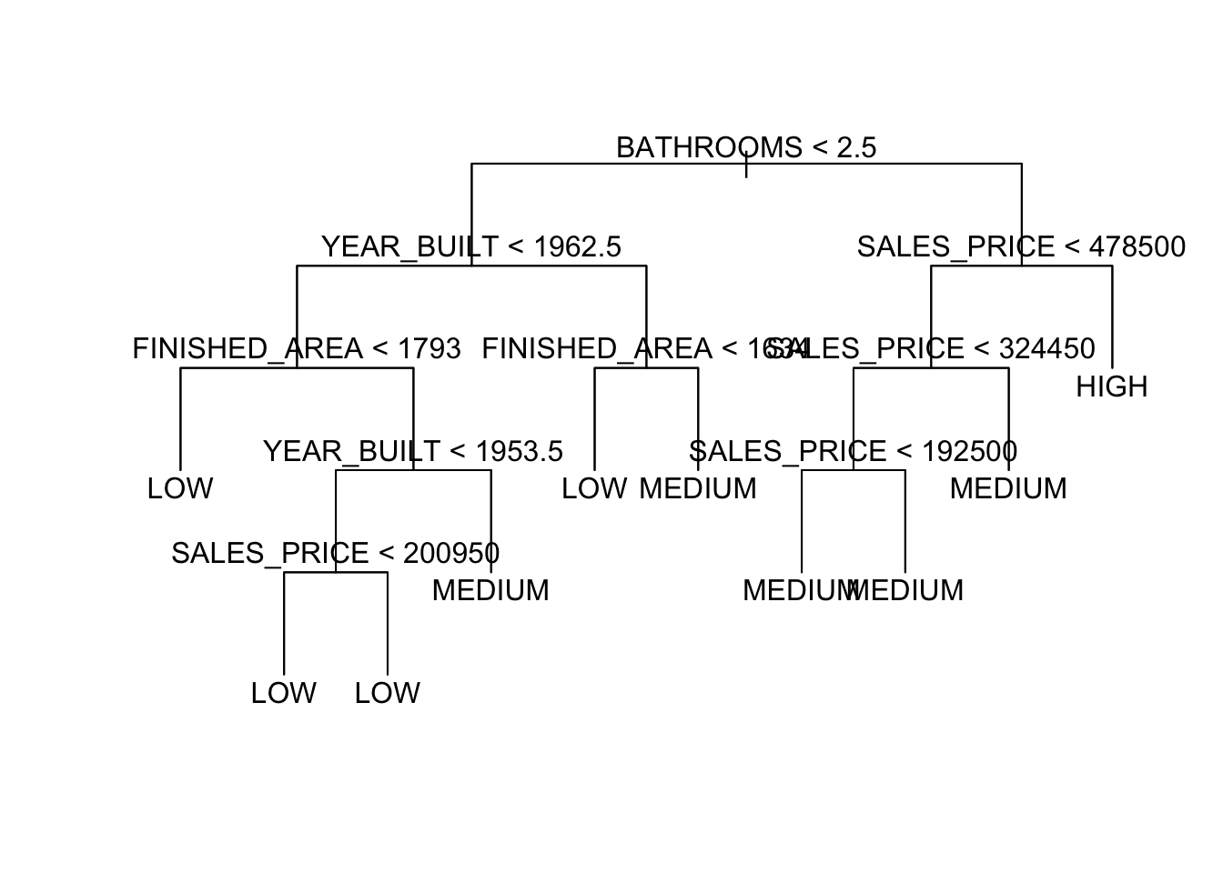
We get a much different tree.
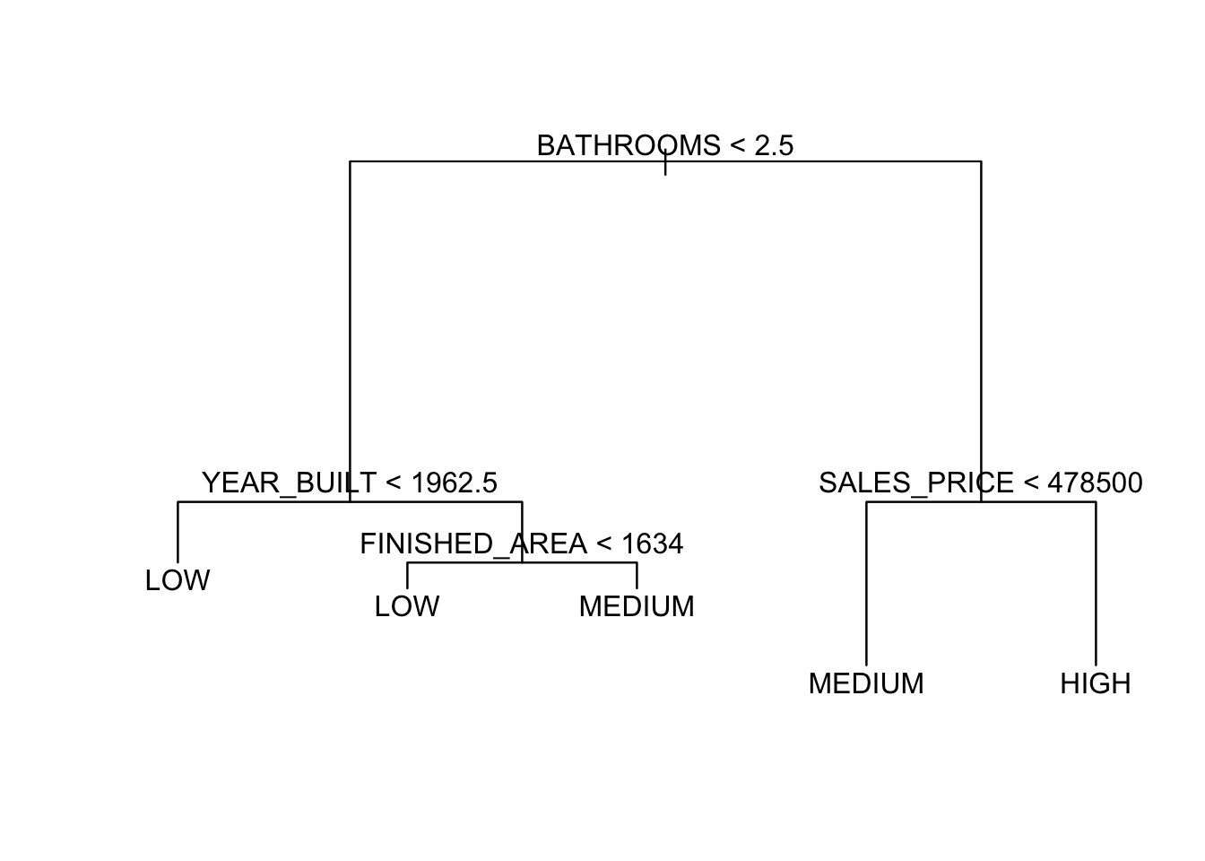
To interpret the tree, start at the top, at the root node.
- The variable at the root node is the one that offers the most contribution to making the prediction.
- The variable is identified as is the threshold for the logical comparison.
- If
TRUE, then go left. - If
FALSEthen go right.
- If
- The height of the vertical lines below each split node indicates the contribution of the split to reducing the “impurity” in the set of resultant leaf nodes.
- You expect the lines to get shorter as you go down the tree.
If you just want to see the results, without the line lengths meaning anything (better readability), you can plot with type = "uniform.
8.4.2 Choosing the Splits
For regression trees, the splits are chosen to maximize the reduction in the error sum of squares explained by the split so the line lengths represent that relative reduction.
- Longer lines means more of the error was explained.
For classification trees, the splits are chosen to maximize the reduction in the Gini Impurity Index across the resultant leaf nodes.
- This index is not quite the same as the Gini Coefficient used in social sciences, e.g., as a measure of income inequality within a population, but it is named after the same mathematician.
- The
tree::tree()function uses the Classification and Regression Trees (CART) algorithm for deciding how to make a split on a classification tree (there are other algorithms). - This algorithm computes the impurity index based on how often a randomly chosen element from the set would be incorrectly labeled if it was randomly labeled according to the distribution of labels in the subset.
- Compute the index \(I_G(p)\) by summing the probability of class \(i\) being chosen, \(p_i\), times the probability of a mistake in categorizing that item \(\sum_{k \neq i}p_{k}=1-p_i\)
- For \(M\) classes, where \(i \in \{1, \ldots, M\}\) and \(p_i\) is the proportion of items labeled with class \(i\) at the node, then calculate the index as:
\[ I_{G}(p) = \sum_{i=1}^{M}\left(p_i\sum_{k\neq i}p_k\right) = 1-\sum_{i=1}^M p_i^2 \]
- Repeat for each node created by the split to make new leaf nodes.
- To get the result for a split, create a weighted sum of the indices across the two resultant leaf nodes where the weights are the number of observations in each leaf node.
\[ I_{G}(Split) = \frac{n_{Left}I_{G}(Left) + n_{Right}I_{G}(Right) }{n_{Left} + n_{Right}} \]
- The algorithm can reuse variables on multiple nodes, but with different thresholds.
- If all the responses at a node are of the same class, then \(p_i = 1\) so \(I_G(p) = 0\) and that node cannot be split any more. That node remains a leaf node.
As more splits occur, the nodes become more pure.
- It is not required that every leaf-node be pure as we may want to tune (trim) to get close enough and avoid overfitting.
An example of Choosing a Split.
A split node has 10 categorical observations as follows.
- Class 1: X1 values: 2, 3, 5
- Class 2: X1 values 3, 5, 7, 8
- Class 3: X1 values 5, 6, 9
What is the probability of each class being chosen?
- Class 1: \(3/(3 + 4 + 3) = 3/10 = 0.3\)
- Class 2: \(4/10 = 0.4\)
- Class 3: \(3/10 = 0.3\)
\(\sum_{i=i}^3p(i) = 1\).
What is the probability of being misclassified?
- Class 1: \((4 + 3)/(10) = 1 - (3/10) = 0.7\)
- Class 2: \((3+3)/10 = 0.6\)
- Class 3: \((3+4)/10 = 0.7\)
So p(misclassified)\(_i\) = \(\sum_{k\neq i}^M p_k\)
What is the Gini Impurity Index for this node?
The Gini index for the node (before split) is the sum of the pairwise probabilities for each class.
\[ \begin{align} I_G(Node) &= \sum_{i=1}^3\left(p_i \sum_{k\neq i}^3(1-p_k)\right) = 1 - \sum_{i=1}^3 p_i^2\\ \\ I_G (Node) &= 1-(.09 +.16 +.09) = 1 - .34 = .66 \end{align} \]
Compare possible splits at X1 \(\leq5\) and X1 \(\leq 6\)
Consider a split at 5
Calculate the impurity (or cost) of each split as a weighted sum of the \(I_G\) for each side.
- Left side of the split (\(X1 \leq5\)) has a total of 3, 2, and 1 observations in each class and the right side (\(X1>5\)) has 0, 2, and 2 observations in each class.
- \(I_G(Left) = 1- ((3/6)^2 + (2/6)^2 + (1/6)^2) = 1 - (9 + 4 + 1)/36 = .61\)
- \(I_G(Right) = 1- ((0/4)^2 + (2/4)^2 + (2/4)^2) = 1 - (0+ 4 + 4)/16 = .5\)
- Combine them in a weighted average to get the Impurity of (split at 5) = \(I_G(5)=(6/10)*.61 + (4/10)*.5 = .566\)
Consider a split at 6
Calculate the impurity (or cost) of each split as a weighted sum of the \(I_G\) for each side.
- Left has 3, 2, 2 observations in each class, Right has 0, 1, 2 observations in each class.
- \(I_G(Left) = 1- ((3/7)^2 + (2/7)^2 + (2/7)^2) = 1 - (9 + 4 + 4)/49 = .65\)
- \(I_G(Right) = 1- ((0/3)^2 + (1/3)^2 + (2/3)^2) = 1 - (0+ 1 + 4)/9 = .56\)
- Combine them in a weighted average to get the Impurity of (split at 6) = \(I_G(6)=(7/10) *.65 + (3/10)*.55 = .62\)
Notice both \(I_G(5)< I_G(Node)\) and \(I_G(6)< I_G(Node)\).
\(I_G(5)=.565 < I_G(6)=.620\) so Split at 5 has less impurity so would choose that one. Would need to compare all the other possible splits (2, 3, 7, 8, 9) as well before making the final choice.
8.4.3 Measuring Performance of Trees in R
The detailed structure of the tree is in the frame element of the tree() output, here tr$frame.
- The default display of the model object shows you the contents of
frame. - It shows the structure using indentation.
- It’s a data frame, but you have to
View()it to see it as a table.
- It’s a data frame, but you have to
- Each row indicates a node on the tree
-
varis variable used at the split. -
nis the number of cases reaching that node (may be weighted). -
devis the deviance remaining at that node. -
yvalis the \(\hat{y}\) that would be predicted if it were a leaf node. - Columns for the number of levels with the associated proportions \(p_i\) at that node.
- Multiplying
nby the proportions gives the number of observations of each level in the node.
- Multiplying
- An asterisk indicates a terminal or leaf node.
node), split, n, deviance, yval, (yprob) * denotes terminal node 1) root 522 997.90 MEDIUM ( 0.130268 0.314176 0.555556 ) 2) BATHROOMS < 2.5 243 326.70 LOW ( 0.004115 0.646091 0.349794 ) 4) YEAR_BUILT < 1962.5 174 180.10 LOW ( 0.000000 0.787356 0.212644 ) 8) FINISHED_AREA < 1793 110 62.30 LOW ( 0.000000 0.918182 0.081818 ) * 9) FINISHED_AREA > 1793 64 87.72 LOW ( 0.000000 0.562500 0.437500 ) 18) YEAR_BUILT < 1953.5 29 29.57 LOW ( 0.000000 0.793103 0.206897 ) 36) SALES_PRICE < 200950 15 0.00 LOW ( 0.000000 1.000000 0.000000 ) * 37) SALES_PRICE > 200950 14 19.12 LOW ( 0.000000 0.571429 0.428571 ) * 19) YEAR_BUILT > 1953.5 35 46.18 MEDIUM ( 0.000000 0.371429 0.628571 ) * 5) YEAR_BUILT > 1962.5 69 92.84 MEDIUM ( 0.014493 0.289855 0.695652 ) 10) FINISHED_AREA < 1634 15 15.01 LOW ( 0.000000 0.800000 0.200000 ) * 11) FINISHED_AREA > 1634 54 54.94 MEDIUM ( 0.018519 0.148148 0.833333 ) * 3) BATHROOMS > 2.5 279 369.10 MEDIUM ( 0.240143 0.025090 0.734767 ) 6) SALES_PRICE < 478500 224 186.40 MEDIUM ( 0.080357 0.031250 0.888393 ) 12) SALES_PRICE < 324450 144 49.88 MEDIUM ( 0.000000 0.041667 0.958333 ) 24) SALES_PRICE < 192500 12 16.30 MEDIUM ( 0.000000 0.416667 0.583333 ) * 25) SALES_PRICE > 192500 132 11.76 MEDIUM ( 0.000000 0.007576 0.992424 ) * 13) SALES_PRICE > 324450 80 95.54 MEDIUM ( 0.225000 0.012500 0.762500 ) * 7) SALES_PRICE > 478500 55 37.91 HIGH ( 0.890909 0.000000 0.109091 ) *- This tree has one pure node. Which one?
-
You can see the summary of the tree model with summary()
- It shows the variables actually used, the residual mean deviance and the Misclassification error rate.
Classification tree:
tree(formula = as.factor(QUALITY) ~ . - ID, data = homes)
Variables actually used in tree construction:
[1] "BATHROOMS" "YEAR_BUILT" "FINISHED_AREA" "SALES_PRICE"
Number of terminal nodes: 10
Residual mean deviance: 0.7013 = 359.1 / 512
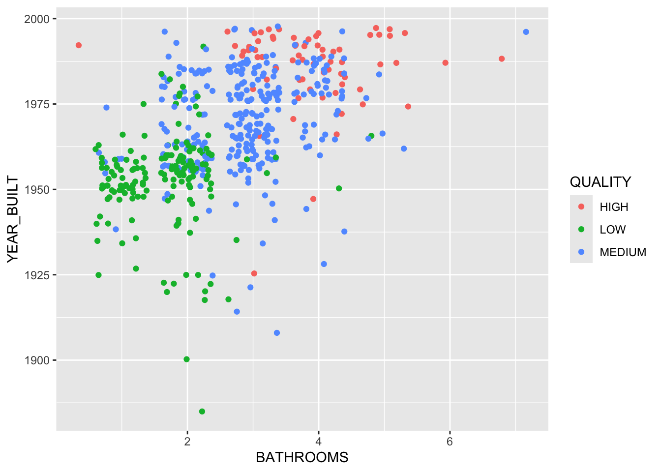
Misclassification error rate: 0.136 = 71 / 522 We can plot the tree results for the two variables.
For two other variables.
Let’s fit a tree with just these two variables.
Show code
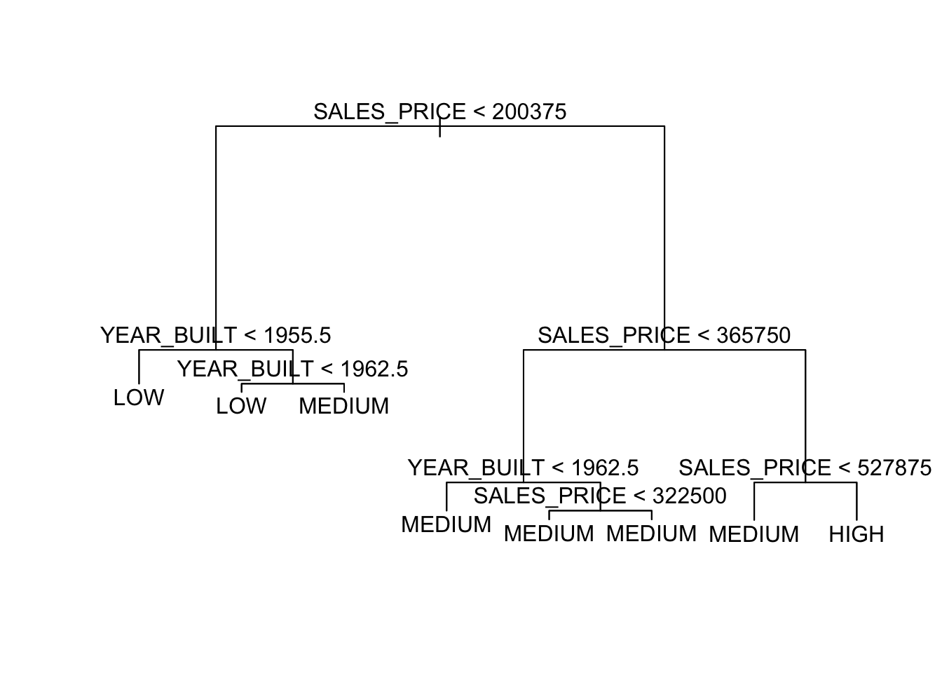
node), split, n, deviance, yval, (yprob)
* denotes terminal node
1) root 522 997.900 MEDIUM ( 0.13027 0.31418 0.55556 )
2) SALES_PRICE < 200375 193 224.900 LOW ( 0.00000 0.73057 0.26943 )
4) YEAR_BUILT < 1955.5 78 25.430 LOW ( 0.00000 0.96154 0.03846 ) *
5) YEAR_BUILT > 1955.5 115 156.900 LOW ( 0.00000 0.57391 0.42609 )
10) YEAR_BUILT < 1962.5 69 84.800 LOW ( 0.00000 0.69565 0.30435 ) *
11) YEAR_BUILT > 1962.5 46 61.580 MEDIUM ( 0.00000 0.39130 0.60870 ) *
3) SALES_PRICE > 200375 329 490.900 MEDIUM ( 0.20669 0.06991 0.72340 )
6) SALES_PRICE < 365750 221 178.700 MEDIUM ( 0.01357 0.10407 0.88235 )
12) YEAR_BUILT < 1962.5 71 84.430 MEDIUM ( 0.00000 0.28169 0.71831 ) *
13) YEAR_BUILT > 1962.5 150 58.700 MEDIUM ( 0.02000 0.02000 0.96000 )
26) SALES_PRICE < 322500 120 28.060 MEDIUM ( 0.00000 0.02500 0.97500 ) *
27) SALES_PRICE > 322500 30 19.500 MEDIUM ( 0.10000 0.00000 0.90000 ) *
7) SALES_PRICE > 365750 108 145.200 HIGH ( 0.60185 0.00000 0.39815 )
14) SALES_PRICE < 527875 67 88.520 MEDIUM ( 0.37313 0.00000 0.62687 ) *
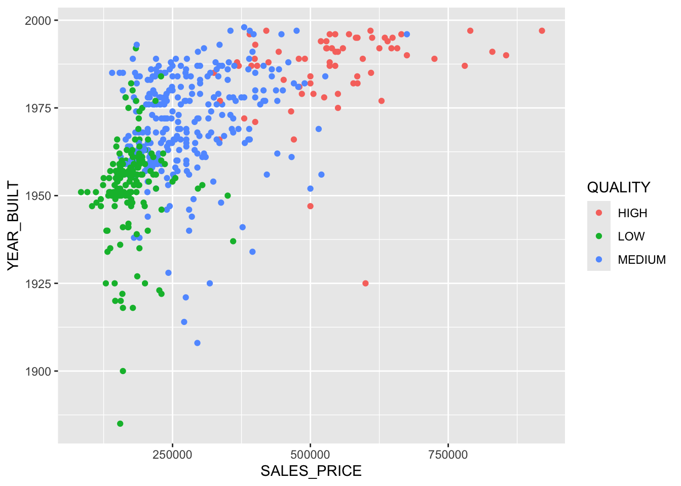
15) SALES_PRICE > 527875 41 9.403 HIGH ( 0.97561 0.00000 0.02439 ) *Now we can see how the splits are separating the space.
Show code
ggplot(homes, aes(SALES_PRICE, YEAR_BUILT, color = QUALITY)) +
geom_point() +
geom_vline(xintercept = 200375, lty = 1, color = "red",
linewidth = 2, alpha = .4) +
geom_vline(xintercept = 365750, lty = 2, color = "brown", linewidth = 1) +
geom_line(data = data.frame(x = c(0, 200375), y = c(1955.5, 1955.5)),
aes(x, y), color = "brown", lty = 2, linewidth = 1)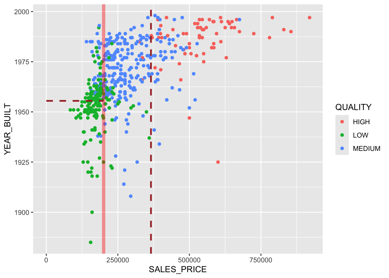
You can see the whole layout with Base R plots and tree::partition.tree().
Show code
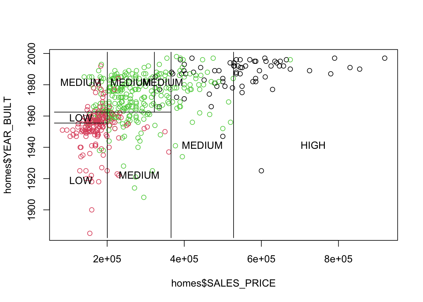
Each rectangle corresponds to a terminal node.
Both representations of the two-variable tree in Figure 8.2 have equal information.
- You can translate from one to the other or create one from the other.
- You can create trees with more than two predictor variables but you cannot plot them as easily.
Show code
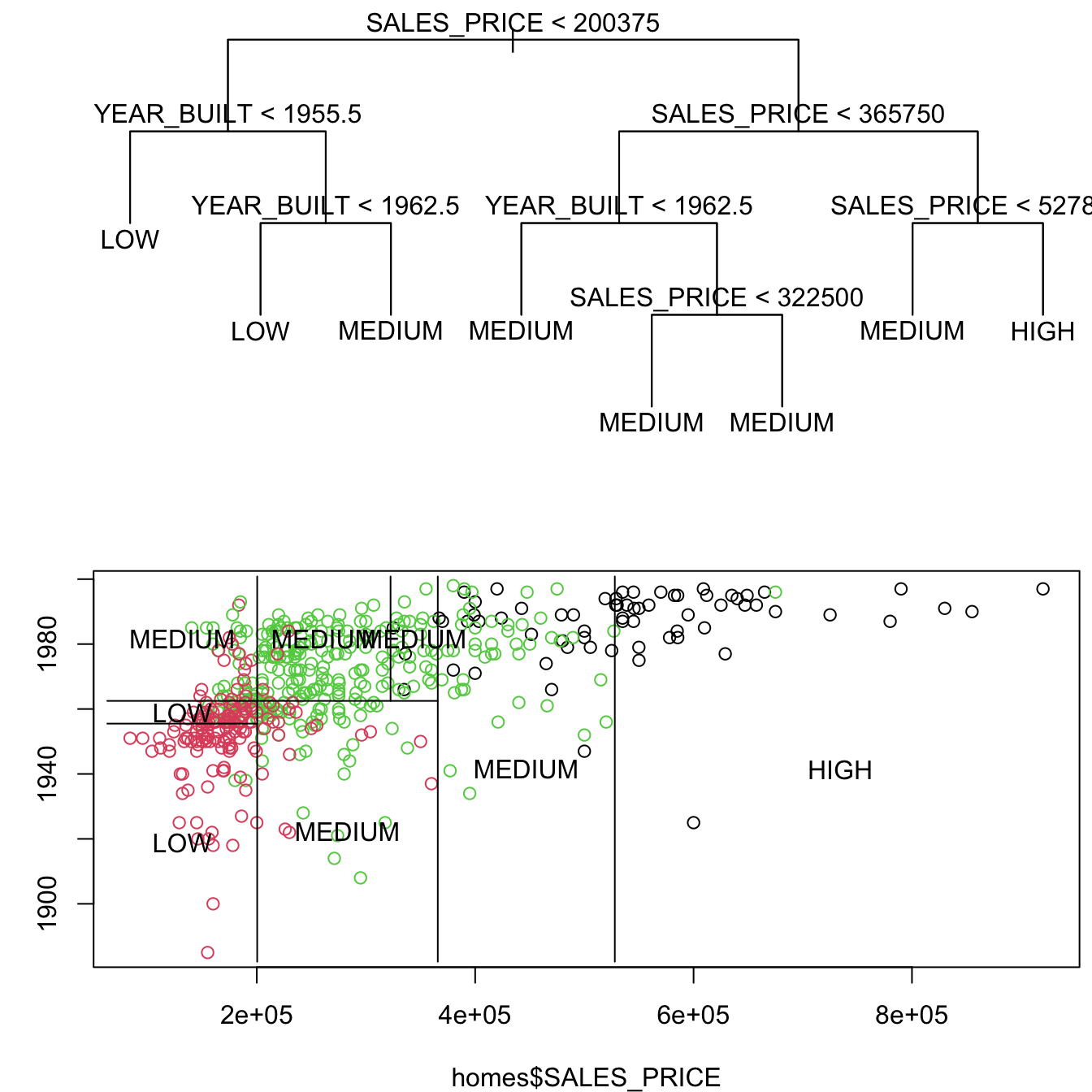
It is straightforward to go from the tree diagram to the plot.
- Start at the top and draw a line matching the variable and threshold of the split.
- Move to the next level and repeat for each branch.
- When you get to a leaf node, label the cell based on the prediction.
It can be more challenging to go from the plot back to the tree as the root may not be obvious at first.
You can see the variables and thresholds.
It is a process of clearly identifying the thresholds along with the lesser-included conditions.
Look for the most common variable and threshold combinations and work down each branch.
-
Label each cell and identify the variables and conditions and decisions. (numbers reduced in digits in what follows)
1. sp \< 2 and yb \> 55 and yb \> 62 = M 2. sp \< 2 and yb \< 55 and yb \< 62 = L 3. sp \< 2 and yb \< 55 = L 4. sp \> 2 and sp \< 3.6 and sp \< 3.2 and yb \> 62 = M 5. sp \> 2 and sp \< 3.6 and sp \< 3.2 and yb \> 62 = M 6. sp \> 2 and sp \< 3.6 and yb \< 62 = M 7. sp \> 2 and sp \> 3.6 and sp \< 5.5 = M 8. sp \> 2 and sp \> 3.6 and sp \> 5.5 = H 8 cells means 7 splits.
-
Reorder them if necessary and look for the most common variable/threshold (with lesser included cases).
- Here we can see
SALES_PRICE< 2 is the root node as it occurs in every case.
- Here we can see
-
For those that are TRUE, go fown that branch and look for the next most common (with lesser included cases).
- Consider
YEAR_BUILT< 55 as the node since 55 < 65.
- Consider
-
Keep working down the branch for cases (1, 2, 3).
- Left side (3): True means Leaf node for
Low - Right side (1, 2): Consider yb < 62, then, not a leaf node, so consider
- Left side (2): True means Leaf node for
Low - Right Side (1): True means Leaf node for
Medium.
- Left side (2): True means Leaf node for
- Left side (3): True means Leaf node for
That completes cases 1, 2, and 3.
Go back to the root node and start working the next layer considering only those decisions not yet mapped out (4, 5, 6, 7, 8).
Look for most common variable/threshold (with lesser included cases).
-
Consider
SALES_PRCE< 3.6. It has three true and two false.- Left side:YB < 62 most common as next split
- Left: Leaf -> Medium
- Right: SP < 3.2
- Left: Leaf -> Medium
- Right: Leaf -> Medium
- That completes 4, 5, 6.
- Right side: sp < 5.5
- Left Leaf -> Medium
- Right Leaf - High
- That completes 7, 8.
- Left side:YB < 62 most common as next split
All splits are now completed.
8.4.4 Tuning the Tree
The algorithm decides what splits to make to maximize the reduction in MSE or the gini impurity index.
We can tune the tree based on how many terminal nodes we want it to have.
We can use cross-validation with a validation set to assess performance.
-
cv.tree()runs \(K\)-fold cross validation with \(K=10\). - When fitting the trees, it also calls
prune.tree()which will trim leaves by recursively “snipping” off the least important splits.
Show code
$size
[1] 10 9 8 7 6 5 4 3 2 1
$dev
[1] 515.6691 513.5611 496.0108 521.9305 521.1874 547.1770 589.7400
[8] 604.4614 721.1613 1003.3119
$k
[1] -Inf 10.44788 11.97109 21.82445 22.89045 30.04703 40.95862
[8] 53.80531 144.81740 302.03830
$method
[1] "deviance"
attr(,"class")
[1] "prune" "tree.sequence"-
sizeis the number of terminal nodes in the tree (in decreasing order left to right). -
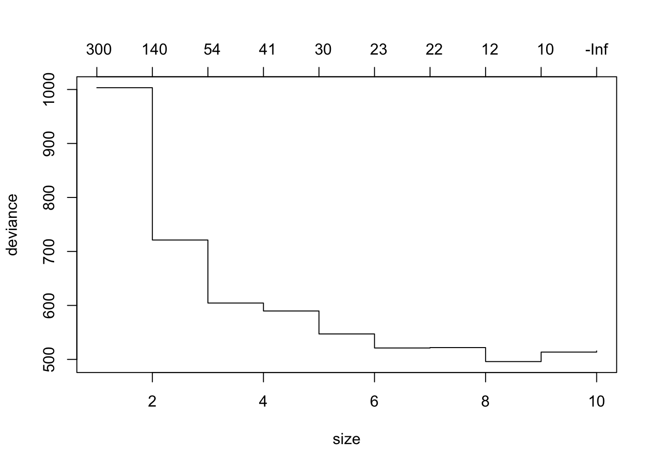
devis the measure of log-likelihood and the lowest number is the best fit. Here that is 8 terminal nodes at 496. -
kis the value of the cost-complexity parameter used byprune.tree()to prune the tree.- This is a tuning parameter of a penalty function used to drive down the number of terminal nodes based on the overall performance of the tree (misclassification rate) and reduce overfitting.
- Similar in concept to \(\lambda\) used in shrinkage methods or adjusted R2 in regression.
- Without it the tree would grow larger and larger while overfitting.
Our initial tree had 10 nodes so the cross validation will only address the nodes in the original tree and fewer.
You can get the tree size with the minimum deviance and also plot the cross validation results.
- The numbers across the top are the values of \(k\), the cost complexity parameter, and
-Infis the default for getting the largest tree possible - with the greatest chance of overfitting.
To see the new, optimal, tree, use prune.tree() with the best number of nodes.
Classification tree:
snip.tree(tree = tr, nodes = 9L)
Variables actually used in tree construction:
[1] "BATHROOMS" "YEAR_BUILT" "FINISHED_AREA" "SALES_PRICE"
Number of terminal nodes: 8
Residual mean deviance: 0.7422 = 381.5 / 514
Misclassification error rate: 0.1533 = 80 / 522 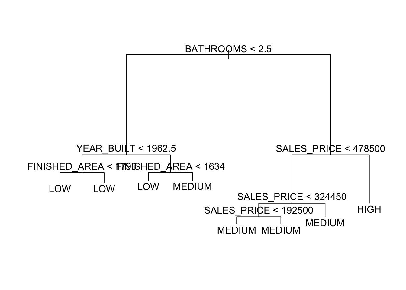
This optimum is based on deviance for regression and classification trees.
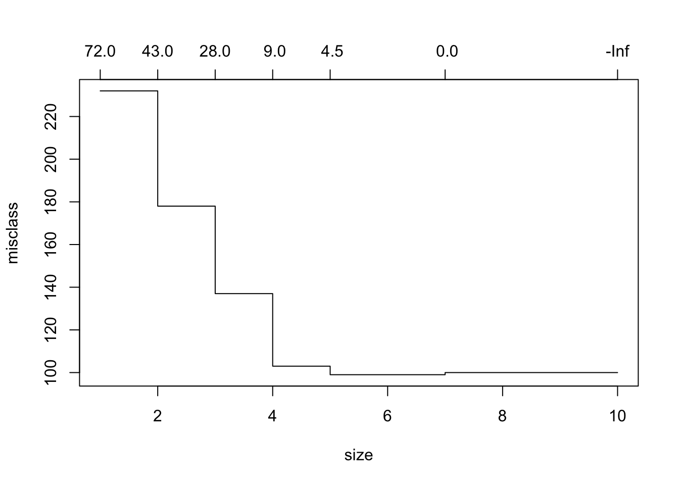
For classification trees only, we can choose to prune based on the misclassification rate.
$size
[1] 10 7 5 4 3 2 1
$dev
[1] 100 100 99 103 137 178 232
$k
[1] -Inf 0.0 4.5 9.0 28.0 43.0 72.0
$method
[1] "misclass"
attr(,"class")
[1] "prune" "tree.sequence"- Here
devis not deviance but the number of misclassified responses.
Here it says to use 5 branches.
8.4.5 Regression Trees in R
Let’s predict SALES_PRICE.
node), split, n, deviance, yval
* denotes terminal node
1) root 522 9.911e+12 277900
2) as.factor(QUALITY): LOW,MEDIUM 454 3.360e+12 238100
4) FINISHED_AREA < 2223.5 307 7.316e+11 196900
8) BATHROOMS < 2.5 223 2.850e+11 180500 *
9) BATHROOMS > 2.5 84 2.279e+11 240300 *
5) FINISHED_AREA > 2223.5 147 1.016e+12 324200
10) FINISHED_AREA < 2818.5 96 3.261e+11 286600 *
11) FINISHED_AREA > 2818.5 51 2.982e+11 395000 *
3) as.factor(QUALITY): HIGH 68 1.031e+12 543600
6) FINISHED_AREA < 3846.5 52 4.568e+11 513600 *
7) FINISHED_AREA > 3846.5 16 3.742e+11 641300
14) YEAR_BUILT < 1989.5 7 9.193e+10 524800 *
15) YEAR_BUILT > 1989.5 9 1.135e+11 731900 *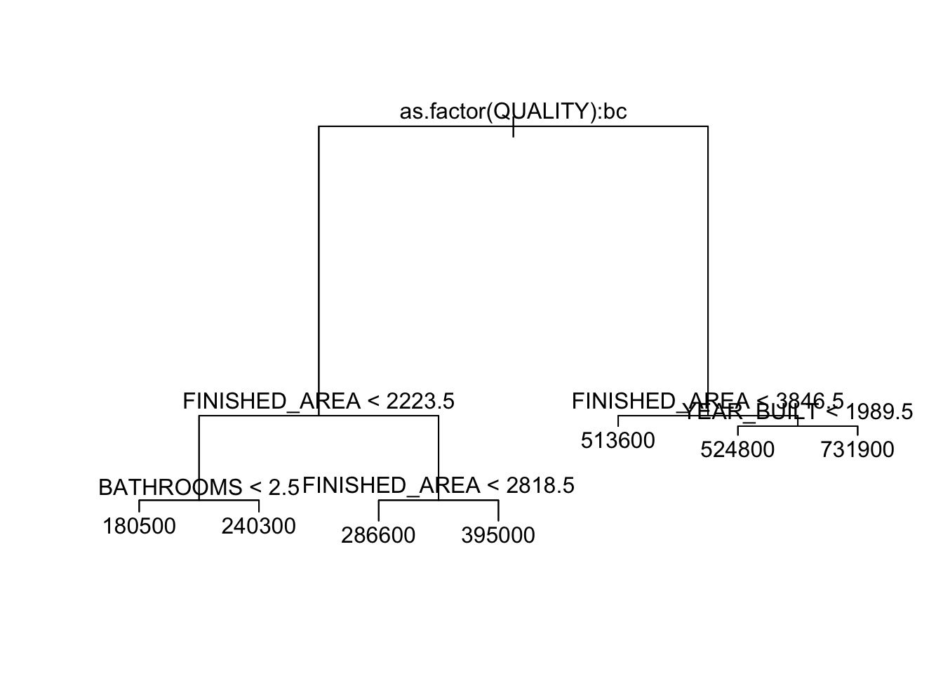
[1] "HIGH" "LOW" "MEDIUM"The terminal nodes each have a \(\hat{y}_m=\bar{y}_m\) as the mean of the price of the houses that were left in the \(m\)th node.
- The root node splits on a categorical variable
QUALITY.- The
bcmeans that to the left (YES) are the second and third levels of theQUALITYvariable (MEDIUMandLOW). andHIGHis to the right (NO).
- The
- Note that it always adds .5 to avoid ties.
- As before, the values in the output for \(k\) and on the top of the plot are the values of the cost complexity parameter, not the cross-fold validation \(K\).
$size
[1] 7 6 5 4 3 2 1
$dev
[1] 2.501469e+12 2.455349e+12 2.665192e+12 2.710722e+12 2.907232e+12
[6] 4.480617e+12 9.947553e+12
$k
[1] -Inf 1.687930e+11 1.996989e+11 2.186610e+11 3.914207e+11
[6] 1.612596e+12 5.520274e+12
$method
[1] "deviance"
attr(,"class")
[1] "prune" "tree.sequence"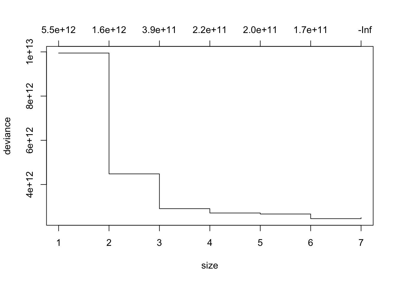
To assess accuracy we will grow many trees and use bootstrap to assess.
- We will look at Bagging (bootstrap aggregation) and then use random selection to minimize correlation (random forests).
8.5 Trees vs. Regression
Regression: \(Y = \beta_0 + \beta_1 X_1 + \cdots\)
Trees: \(Y = \beta_1 I_{A_1} + \beta_2 I_{A_2}\cdots\) splits the \(X\) into regions \(A_j\).
Regression and Trees all fall into the set of base functions we could use for the splines.
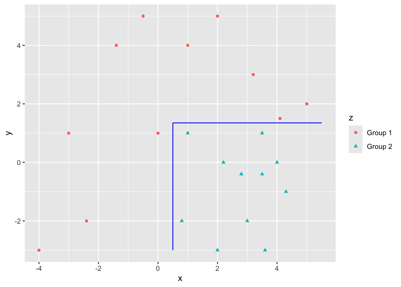
If your data looks like the following, regression works well to separate.
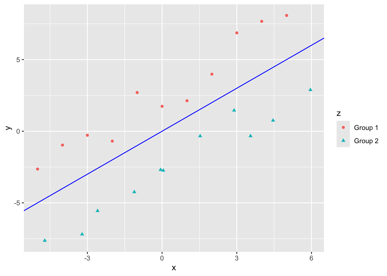
If your data looks like this, regression does not do as well.
- But trees can split the data nicely for a good fit
8.6 Example: Titanic Data
Let’s load the {DALEX} titanic data set.
[1] "gender" "age" "class" "embarked" "country" "fare" "sibsp"
[8] "parch" "survived"- See
?DALEX::titanicfor variable definitions.
We predicted survival using other methods. Let’s try a tree.
Error in tree(survived ~ ., data = titanic): factor predictors must have at most 32 levelsLet’s check out the source of the error.
Rows: 2,207
Columns: 9
$ gender <fct> male, male, male, female, female, male, male, female, male, m…
$ age <dbl> 42.0000000, 13.0000000, 16.0000000, 39.0000000, 16.0000000, 2…
$ class <fct> 3rd, 3rd, 3rd, 3rd, 3rd, 3rd, 2nd, 2nd, 3rd, 3rd, 3rd, 3rd, 3…
$ embarked <fct> Southampton, Southampton, Southampton, Southampton, Southampt…
$ country <fct> United States, United States, United States, England, Norway,…
$ fare <dbl> 7.1100, 20.0500, 20.0500, 20.0500, 7.1300, 7.1300, 24.0000, 2…
$ sibsp <dbl> 0, 0, 1, 1, 0, 0, 1, 1, 0, 0, 0, 0, 1, 0, 0, 0, 0, 0, 0, 0, 0…
$ parch <dbl> 0, 2, 1, 1, 0, 0, 0, 0, 0, 0, 0, 0, 0, 1, 1, 0, 0, 0, 0, 0, 0…
$ survived <fct> no, no, no, yes, yes, yes, no, yes, yes, yes, no, no, no, yes… [1] "Argentina" "Australia" "Austria"
[4] "Belgium" "Bosnia" "Bulgaria"
[7] "Canada" "Channel Islands" "China/Hong Kong"
[10] "Croatia" "Croatia (Modern)" "Cuba"
[13] "Denmark" "Egypt" "England"
[16] "Finland" "France" "Germany"
[19] "Greece" "Hungary" "India"
[22] "Ireland" "Italy" "Japan"
[25] "Latvia" "Lebanon" "Mexico"
[28] "Netherlands" "Northern Ireland" "Norway"
[31] "Peru" "Poland" "Russia"
[34] "Scotland" "Siam" "Slovakia (Modern day)"
[37] "Slovenia" "South Africa" "Spain"
[40] "Sweden" "Switzerland" "Syria"
[43] "Turkey" "United States" "Uruguay"
[46] "Wales" "Yugoslavia" "Guyana" We can eliminate country from the model and try again.
Let’s use three different approaches to removing country from the model
- Remove from the model formula.
- Don’t add into the model.
- Remove from the data frame.
Show code
node), split, n, deviance, yval, (yprob)
* denotes terminal node
1) root 2099 2645.000 no ( 0.67556 0.32444 )
2) gender: female 464 536.700 yes ( 0.26509 0.73491 )
4) class: 3rd 207 287.000 no ( 0.50242 0.49758 ) *
5) class: 1st,2nd,restaurant staff,victualling crew 257 135.500 yes ( 0.07393 0.92607 ) *
3) gender: male 1635 1672.000 no ( 0.79205 0.20795 )
6) class: 2nd,3rd,engineering crew,restaurant staff,victualling crew 1400 1273.000 no ( 0.83071 0.16929 )
12) age < 9.5 44 60.910 yes ( 0.47727 0.52273 )
24) sibsp < 2.5 27 25.870 yes ( 0.18519 0.81481 ) *
25) sibsp > 2.5 17 7.606 no ( 0.94118 0.05882 ) *
13) age > 9.5 1356 1183.000 no ( 0.84218 0.15782 ) *
7) class: 1st,deck crew 235 322.200 no ( 0.56170 0.43830 )
14) age < 54.5 201 278.600 yes ( 0.49751 0.50249 ) *
15) age > 54.5 34 15.210 no ( 0.94118 0.05882 ) *node), split, n, deviance, yval, (yprob)
* denotes terminal node
1) root 2179 2749.000 no ( 0.67462 0.32538 )
2) gender: female 489 566.300 yes ( 0.26585 0.73415 )
4) class: 3rd 216 299.400 no ( 0.50926 0.49074 )
8) fare < 23.07 183 250.800 yes ( 0.43716 0.56284 ) *
9) fare > 23.07 33 20.110 no ( 0.90909 0.09091 ) *
5) class: 1st,2nd,restaurant staff,victualling crew 273 143.000 yes ( 0.07326 0.92674 ) *
3) gender: male 1690 1724.000 no ( 0.79290 0.20710 )
6) class: 2nd,3rd,engineering crew,restaurant staff,victualling crew 1451 1321.000 no ( 0.83046 0.16954 )
12) age < 9.5 47 64.960 yes ( 0.46809 0.53191 )
24) sibsp < 2.5 29 26.660 yes ( 0.17241 0.82759 ) *
25) sibsp > 2.5 18 7.724 no ( 0.94444 0.05556 ) *
13) age > 9.5 1404 1222.000 no ( 0.84259 0.15741 ) *
7) class: 1st,deck crew 239 327.300 no ( 0.56485 0.43515 )
14) age < 54.5 205 284.200 no ( 0.50244 0.49756 ) *
15) age > 54.5 34 15.210 no ( 0.94118 0.05882 ) *What do you notice?
Let’s plot the trees - What do you notice?
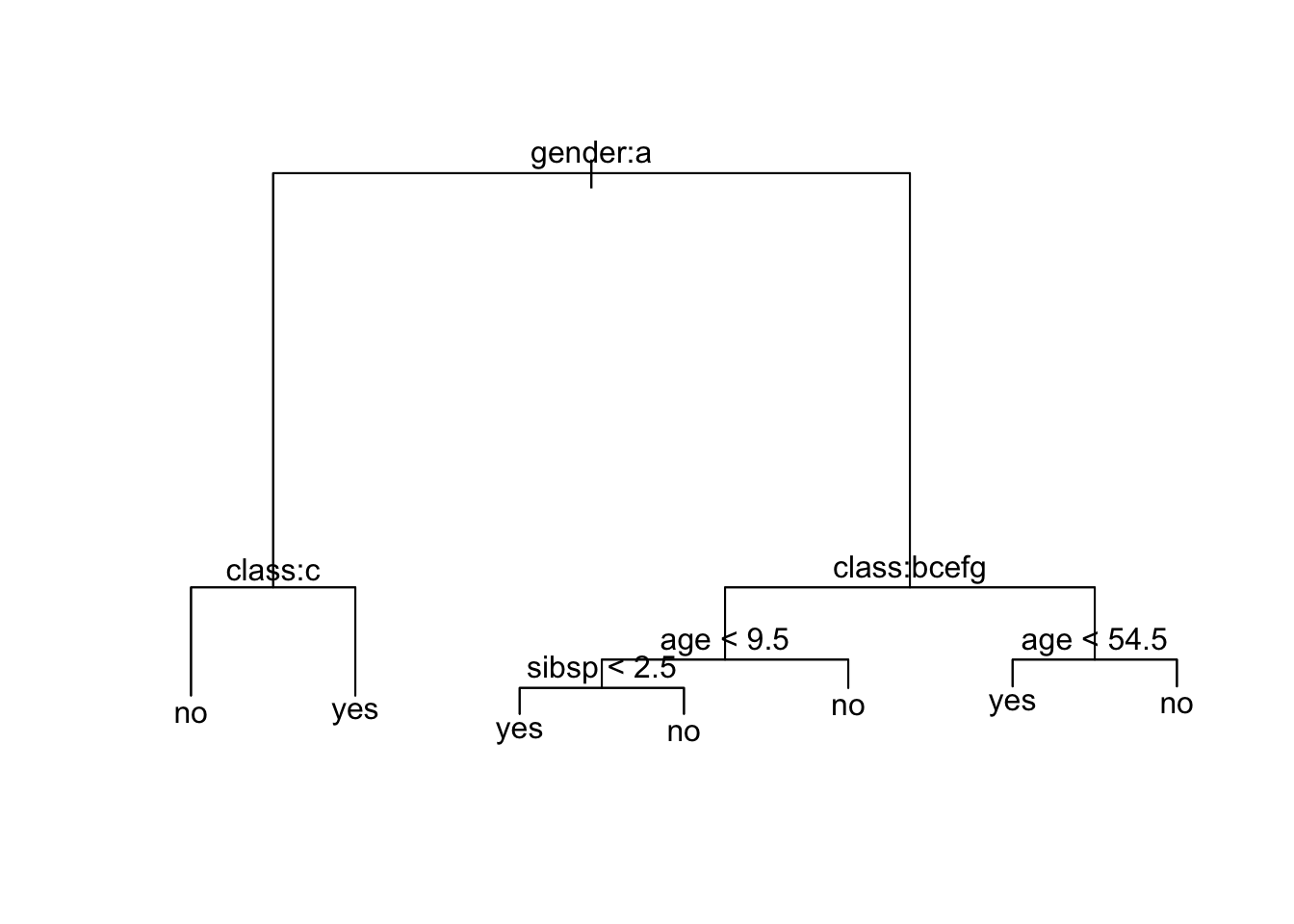
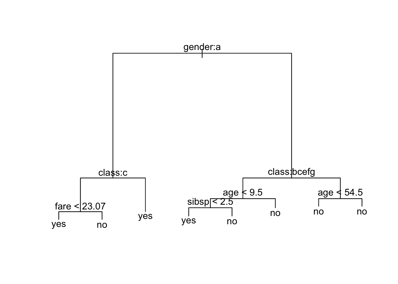
What is going on?
gender age class embarked
female: 489 Min. : 0.1667 1st :324 Belfast : 197
male :1718 1st Qu.:22.0000 2nd :284 Cherbourg : 271
Median :29.0000 3rd :709 Queenstown : 123
Mean :30.4367 deck crew : 66 Southampton:1616
3rd Qu.:38.0000 engineering crew:324
Max. :74.0000 restaurant staff: 69
NA's :2 victualling crew:431
country fare sibsp parch
England :1125 Min. : 0.000 Min. :0.0000 Min. :0.0000
United States: 264 1st Qu.: 0.000 1st Qu.:0.0000 1st Qu.:0.0000
Ireland : 137 Median : 7.151 Median :0.0000 Median :0.0000
Sweden : 105 Mean : 19.773 Mean :0.2972 Mean :0.2294
Lebanon : 71 3rd Qu.: 20.111 3rd Qu.:0.0000 3rd Qu.:0.0000
(Other) : 424 Max. :512.061 Max. :8.0000 Max. :9.0000
NA's : 81 NA's :26 NA's :10 NA's :10
survived
no :1496
yes: 711
Note the number of NAs in country.
Show code
[1] 2179Let’s use the tree model with the most data (the 80 extra rows of data).
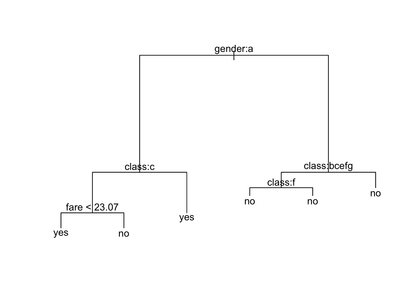
Recall the height of the line for each split is proportional to the amount of SSE (regression) or deviance (classification) explained by the split.
It shows gender is most important predictor for survival.
- The
ameans the first level of the factor variable which here is female.
Since the left side of the split is always the “Yes” answer to the criterion, if you are female then you go down the left branch of the tree.
- Both female and male have the next split as
class, but they have different criteria.
[1] "1st" "2nd" "3rd" "deck crew"
[5] "engineering crew" "restaurant staff" "victualling crew"If female and 3rd class, then not expected to survive.
# A tibble: 9 × 3
# Groups: class [5]
class survived n
<fct> <fct> <int>
1 1st no 5
2 1st yes 139
3 2nd no 12
4 2nd yes 94
5 3rd no 110
6 3rd yes 106
7 restaurant staff yes 2
8 victualling crew no 3
9 victualling crew yes 18If male and any class other than 1st or deck crew, survival depends upon your age and then the number of siblings and parents on board. Otherwise just your age.
gender age class embarked
female: 489 Min. : 0.1667 1st :324 Belfast : 197
male :1718 1st Qu.:22.0000 2nd :284 Cherbourg : 271
Median :29.0000 3rd :709 Queenstown : 123
Mean :30.4367 deck crew : 66 Southampton:1616
3rd Qu.:38.0000 engineering crew:324
Max. :74.0000 restaurant staff: 69
NA's :2 victualling crew:431
country fare sibsp parch
England :1125 Min. : 0.000 Min. :0.0000 Min. :0.0000
United States: 264 1st Qu.: 0.000 1st Qu.:0.0000 1st Qu.:0.0000
Ireland : 137 Median : 7.151 Median :0.0000 Median :0.0000
Sweden : 105 Mean : 19.773 Mean :0.2972 Mean :0.2294
Lebanon : 71 3rd Qu.: 20.111 3rd Qu.:0.0000 3rd Qu.:0.0000
(Other) : 424 Max. :512.061 Max. :8.0000 Max. :9.0000
NA's : 81 NA's :26 NA's :10 NA's :10
survived
no :1496
yes: 711
This is a model built on all the data. Let’s create a validation set to see how well we can predict.
- To ensure we have the same lengths of data we will eliminate records with
NAs since thetree()will eliminate them from the training data.
[1] 2179Show code
node), split, n, deviance, yval, (yprob)
* denotes terminal node
1) root 1089 1393.00 no ( 0.66208 0.33792 )
2) gender: female 256 302.30 yes ( 0.27734 0.72266 )
4) class: 3rd 109 150.00 no ( 0.55046 0.44954 )
8) fare < 23.07 89 122.50 yes ( 0.44944 0.55056 ) *
9) fare > 23.07 20 0.00 no ( 1.00000 0.00000 ) *
5) class: 1st,2nd,restaurant staff,victualling crew 147 78.19 yes ( 0.07483 0.92517 ) *
3) gender: male 833 877.20 no ( 0.78031 0.21969 )
6) class: 2nd,3rd,engineering crew,restaurant staff,victualling crew 720 694.90 no ( 0.81250 0.18750 )
12) class: restaurant staff 34 0.00 no ( 1.00000 0.00000 ) *
13) class: 2nd,3rd,engineering crew,victualling crew 686 680.40 no ( 0.80321 0.19679 ) *
7) class: 1st,deck crew 113 154.10 no ( 0.57522 0.42478 ) *The tree looks a little different.
Let’s predict
no yes
Min. :0.07483 Min. :0.0000
1st Qu.:0.57522 1st Qu.:0.1968
Median :0.80321 Median :0.1968
Mean :0.67045 Mean :0.3295
3rd Qu.:0.80321 3rd Qu.:0.4248
Max. :1.00000 Max. :0.9252 Note these are numeric. This is the summary of the sample proportions at each node, the probabilities.
To get the classifications we have to change the type of prediction for predict.tree()
So now we want to compare predicted responses against the actual testing responses.
To get the prediction error rate we take the proportion of incorrect responses.
8.7 Example: Titanic Data with Package {rpart}
The tree::tree() function is easy to use but does have some limitations.
- It does not handle missing values.
- Character variables must be converted to factors.
- It is limited to only 32 levels for factors.
- It does not handle non-syntactic variable names, e.g.
my var.- You can replace with
names(my_df) <- stringr::str_replace_all(names(my_df), " ", "_")
- You can replace with
- It does not handle data.frames with the name
df(see stackoverflow)
The {rpart} package provides an alternative to the {tree} package.
See the Vingette for examples.
- The {rpart} package is based on the same fundamental algorithms as {tree} but does not have the limitations in
tree::tree(). - It also has some alternative plots provided by the {rpart.plot} package.
Tree algorithms can run for a long time if you have multiple variables with many levels (more than 10) as every possible level must be checked at each split.
Show code
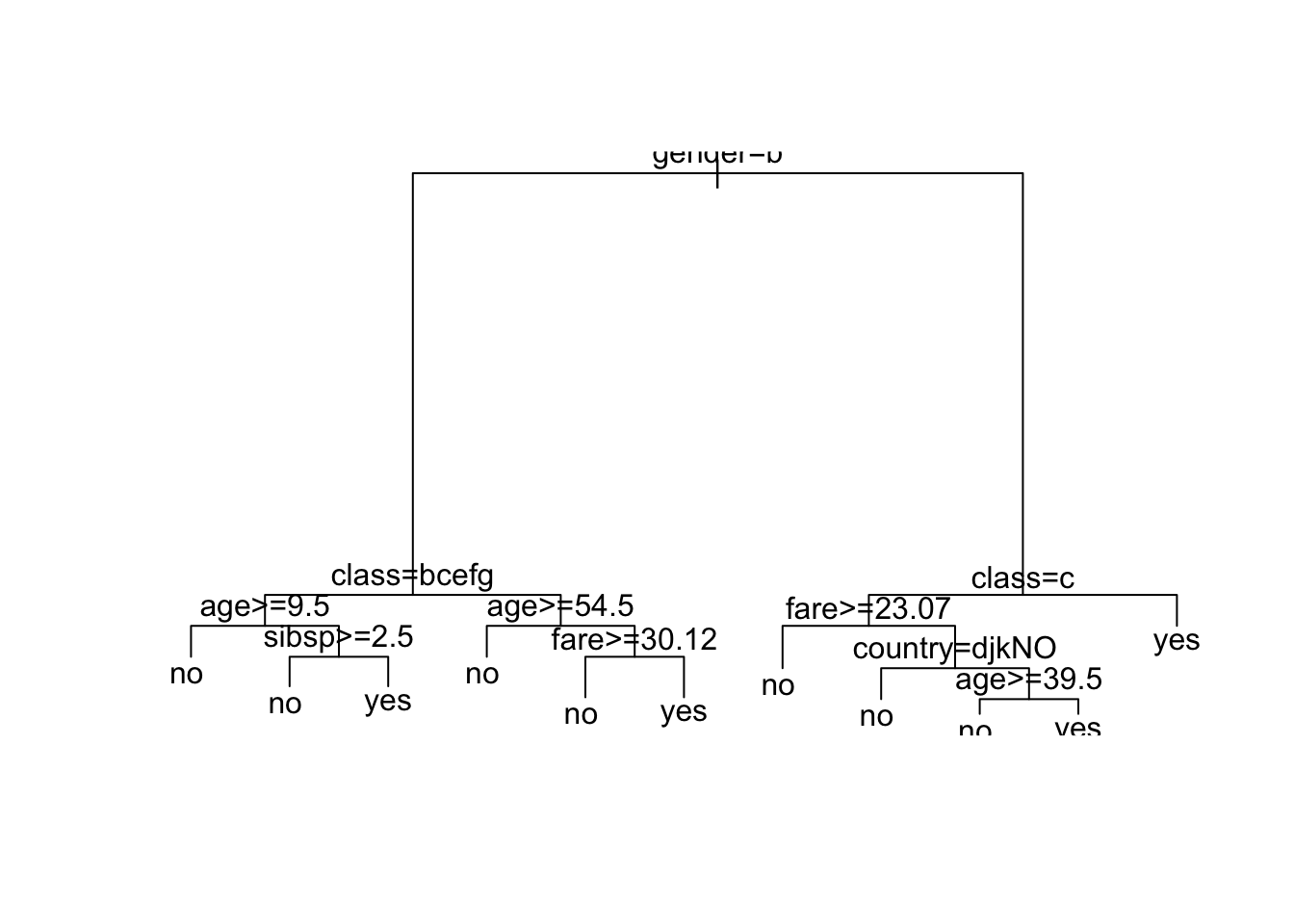
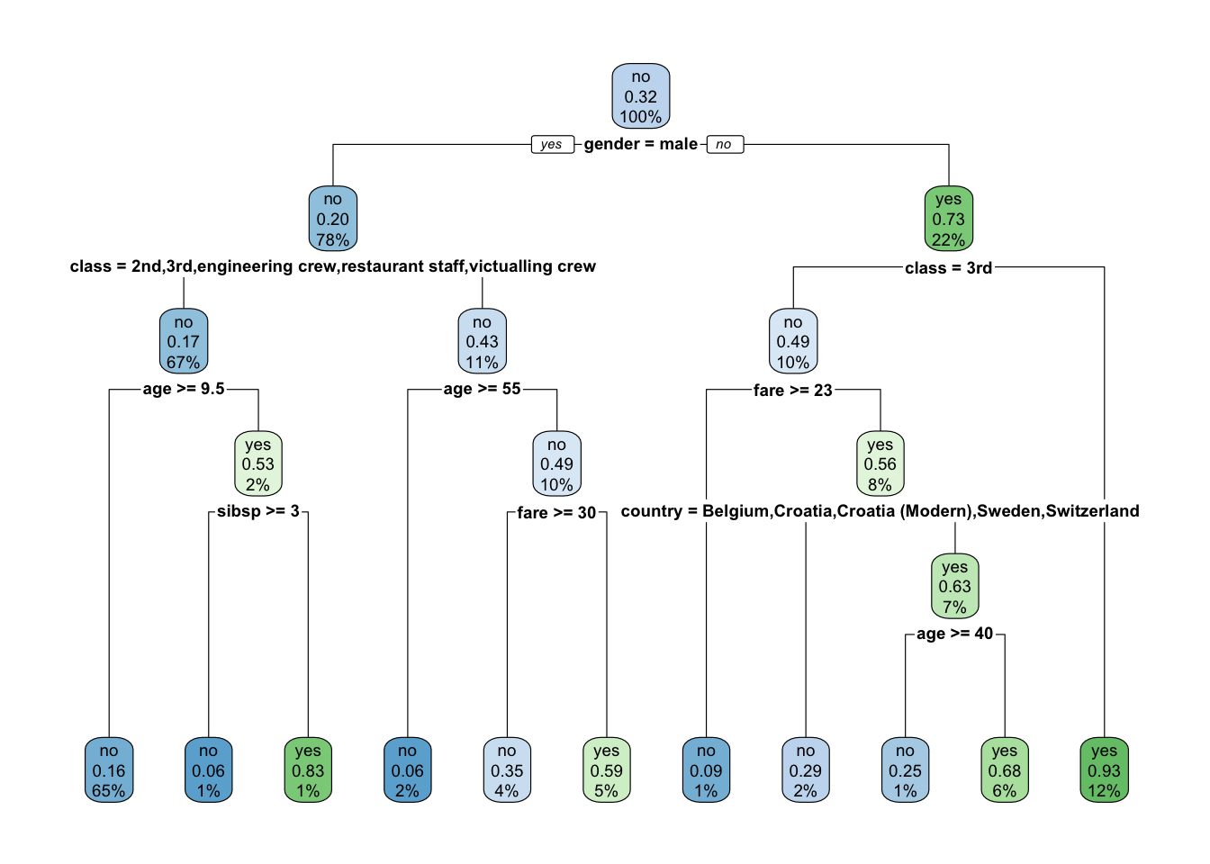
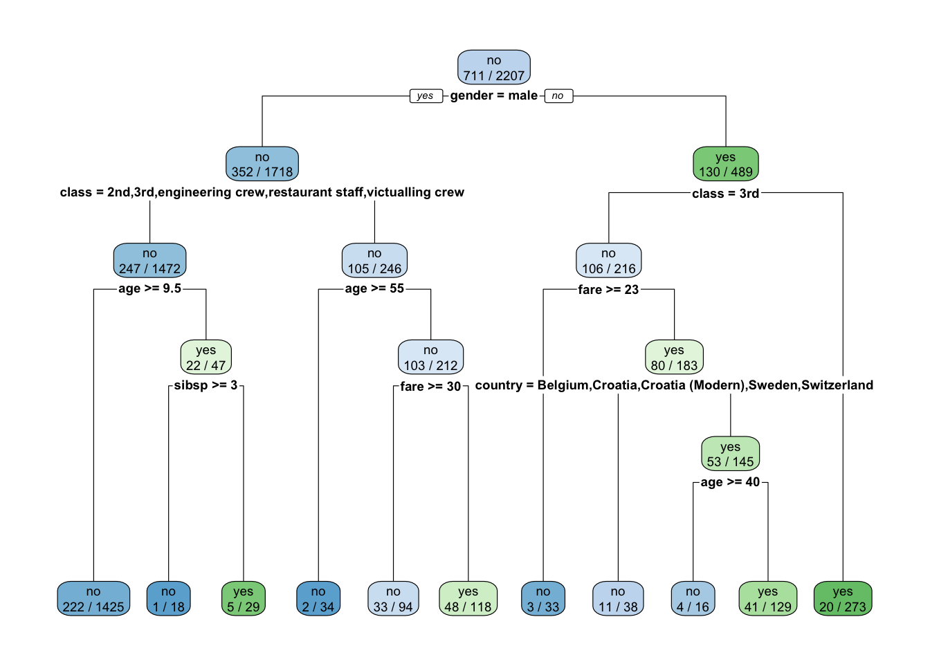
Now the top split is on male and country is in the tree.
It might be easier to see with the different plot.
- The Second class for the node.
- The probability of the second class.
- Percent of observations at that level in the node.
- You can adjust with the
extraargument.
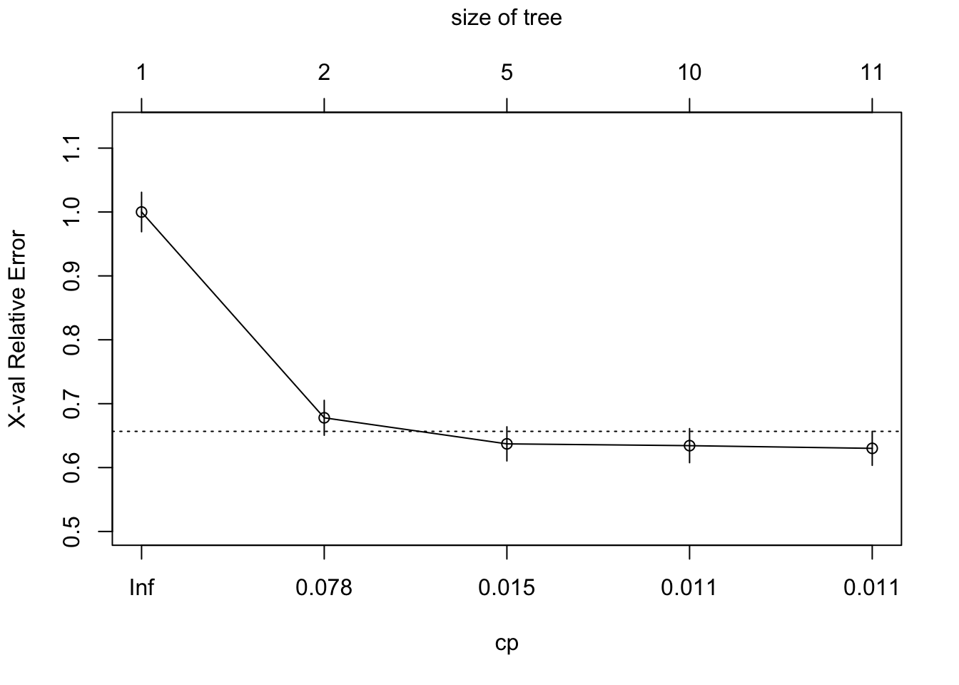
The fitting uses 10-fold cross validation by default to support later pruning.
- You can plot the cross validation with pruning results with
plotcp().
- The results can be found in
$cptable.-
xerroris the scaled (relative) error of the various trees. It is scaled so the largest is 1.0. -
cpis the scaled complexity parameter.
-
CP nsplit rel error xerror xstd
1 0.32208158 0 1.0000000 1.0000000 0.03087663
2 0.01898734 1 0.6779184 0.6779184 0.02729904
3 0.01153305 4 0.6174402 0.6371308 0.02668659
4 0.01125176 9 0.5597750 0.6343179 0.02664279
5 0.01000000 10 0.5485232 0.6300985 0.02657671[1] 0.01Now you can create the pruned tree, which in this case is what we had in the beginning as the default for cp is .01.
Let’s create the validation set and check performance.
[1] 2207set.seed(123)
Z <- sample(nrow(titanic), nrow(titanic)/2)
trpv <- rpart(survived ~ ., data = titanic, subset = Z)
rpart.plot(trpv, faclen = 2, clip.facs = TRUE)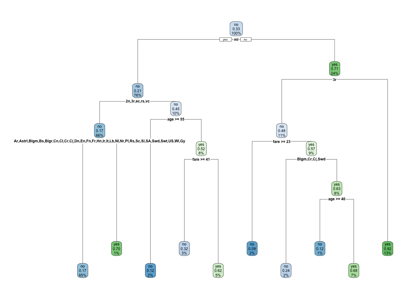
no yes
836 268
Yhat no yes
no 690 146
yes 68 200[1] 0.1938406(table(Yhat, titanic$survived[-Z])[1, 2] +
table(Yhat, titanic$survived[-Z])[2, 1]) /
sum(table(Yhat, titanic$survived[-Z]))[1] 0.1938406So using {rpart} to be able to include country resulted in a slightly better model.
Binary Decision Trees are a popular method as they are easy to interpret and explain to others.
However, they are not always the most accurate.
- They are restrictive as they split the \(X\) space into a fixed set of splits where you have the same prediction for every observation in the region created by a split.
- They can also have high variance as a single value can be influential on which variables are split and the split criteria values.
- A common method for reducing variance is to average results from a number of examples, here multiple trees. This leads us to Bagging.
8.8 Bagging
Bagging (Bootstrap Aggregation) is a method for using Bootstrap to create many trees and average their predictions for each \(X_i\).
Even though we have one set of data, we can use Bootstrap methods to draw many thousands of samples and fit a tree to each sample.
That gives thousands of trees (a forest), each of which has a set of predicted values \(\hat{y}_{it}\) where
- \(i = 1, \ldots, n\) where \(n\) is the sample size and
- \(t = 1, \ldots, B\) where \(B\) is the number of Bootstrap trees that were generated.
With \(B\) samples, we have \(B\) trees, many which may be similar and some that will be different, so we have \(B\) predictions for each observation \(i\) in the data set.
We can then predict \(\hat{y}_i\) in regression trees by
\[ \hat{y}_i = \frac{1}{B}\sum_{t = 1}^B\hat{y}_{it} \]
In classification trees we choose the category with the highest proportion (the mode) as our prediction.
8.8.1 Example of Bagging in R
There are over 20 random forest packages in R.
We will use the package {randomForest}.
Use randomForest() to build a forest (we will use the data without rows with missing data).
data("titanic", package = "DALEX")
titanic2 <- titanic[, !(names(titanic) %in% "country")]
titanicZ <- na.omit(titanic2)
BAG <- randomForest(survived ~ gender + age + class + embarked +
fare + sibsp + parch,
data = titanicZ )
BAG
Call:
randomForest(formula = survived ~ gender + age + class + embarked + fare + sibsp + parch, data = titanicZ)
Type of random forest: classification
Number of trees: 500
No. of variables tried at each split: 2
OOB estimate of error rate: 18.86%
Confusion matrix:
no yes class.error
no 1367 103 0.07006803
yes 308 401 0.43441467- The output shows the number of trees that were built, here 500.
- The
No of variables tried at each split:is only 2 here.- That is because by default this function implements a random forest method which we will talk about next.
- It also provides an
OOB estimate of the error ratewhich we will also discuss. - The confusion matrix includes the
class.errorfor each class based on OOB data: the False Negatives and the False positive Rates.
Let’s rerun but make all seven variables available for each split node by specifying mtry=7.
BAG <- randomForest(survived ~ gender + age + class + embarked +
fare + sibsp + parch,
mtry = 7,
data = titanicZ)
BAG
Call:
randomForest(formula = survived ~ gender + age + class + embarked + fare + sibsp + parch, data = titanicZ, mtry = 7)
Type of random forest: classification
Number of trees: 500
No. of variables tried at each split: 7
OOB estimate of error rate: 21.11%
Confusion matrix:
no yes class.error
no 1315 155 0.1054422
yes 305 404 0.4301834Notice our error rate went up to 21.11% from the default approach 18.68%.
Predicting on all the data shows the training error rate looks pretty good.
Yhat no yes
no 1457 162
yes 13 547[1] 0.08031207Let’s use the same validation subsets as before to get a predictive error rate while forcing it to consider all the variables for each split.
set.seed(123)
Z <- sample(nrow(titanicZ), nrow(titanicZ)/2)
BAG <- randomForest(survived ~ gender + age + class + embarked +
fare + sibsp + parch,
mtry = 7, data = titanicZ[Z,] )
BAG
Call:
randomForest(formula = survived ~ gender + age + class + embarked + fare + sibsp + parch, data = titanicZ[Z, ], mtry = 7)
Type of random forest: classification
Number of trees: 500
No. of variables tried at each split: 7
OOB estimate of error rate: 24.24%
Confusion matrix:
no yes class.error
no 630 91 0.1262136
yes 173 195 0.4701087Let’s predict.
Yhat no yes
no 672 130
yes 77 211[1] 0.1899083Our prediction error rate was higher at 0.189 compared to the training rate of 0.145.
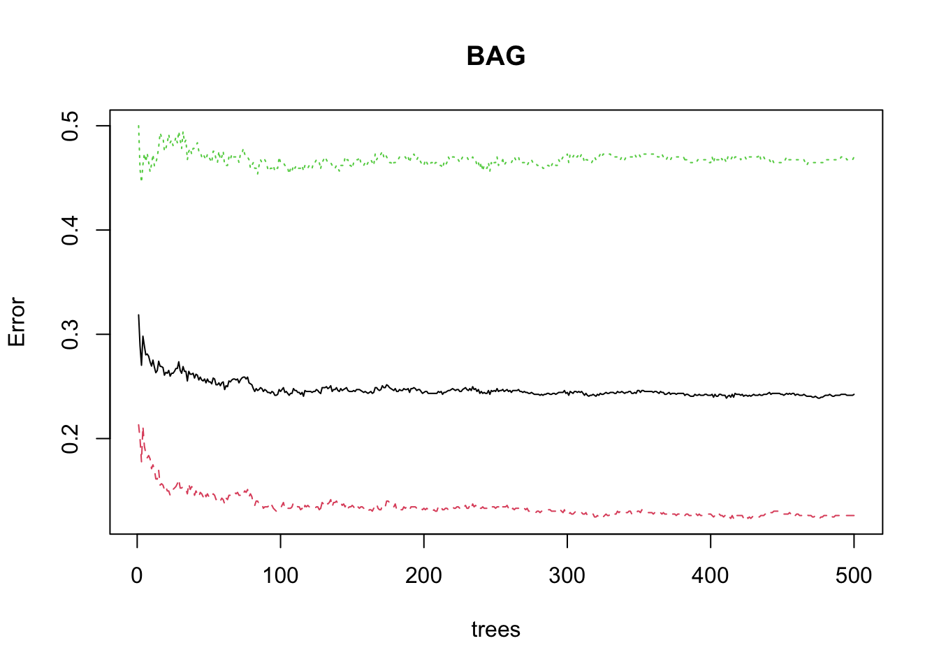
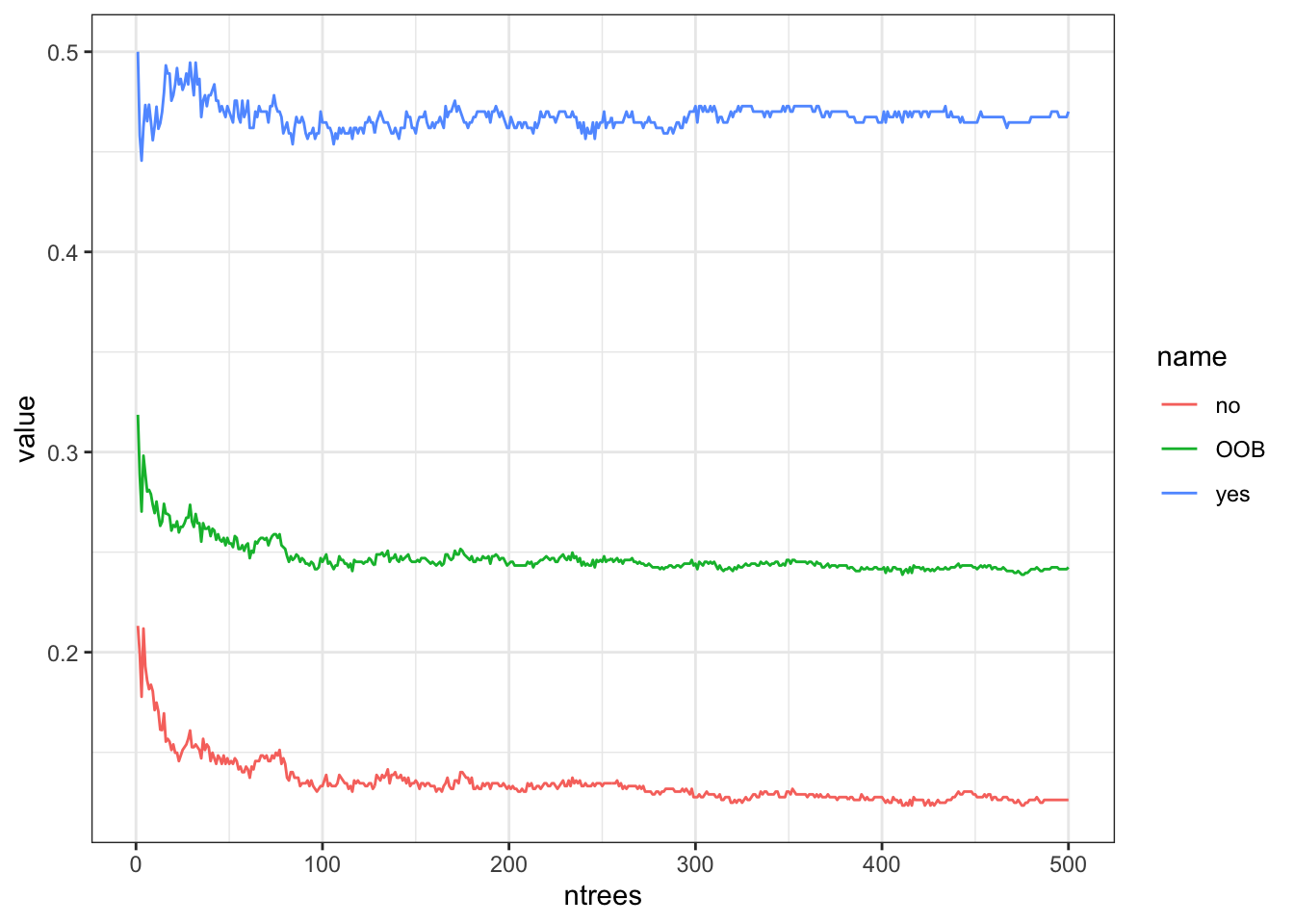
The number of trees is a tuning parameter.
We can plot the Error rate against the number of trees to see where it settles down.
- For classification trees, the
BAGobject includes theerr.rateas a matrix of the OOB andNoandYeserror rates. - The
OOBis the average of theYesandNoerror rates for each tree.
This shows the minimum OOB error was at 411 trees.
8.8.2 OOB - Out of Bag Error Rate
Recall that bootstrap is sampling with replacement so anytime observations are repeated in the sample, that means other observations are left out.
These are the Out of Bag observations.
The randomForest() output tells us how many times an observation was left out of the bag across the total number of trees.
[1] 188 179 179 189 197 190 168 193 199 199 189 183 182 180 195 171 178 187 165
[20] 179 183 185 189 184 167 191 194 186 170 184These OOB observations were used to compute the error rate for that sample since they were Not included in building the tree - they were out of the BAG of training data.
How many sampling units are typically OOB (not included) in a given bootstrap sample? Is it enough to create a meaningful test data set?
- For a bootstrap sample we draw \(n\) units with replacement.
- If observation \(i\) is excluded (OOB), then we can calculate the probability that occurred.
- Each time a given observation is included with probability \(1/n\) so the complement is it is excluded with probability \(1 - 1/n\).
- The probability \(i\) is excluded from an entire bootstrap sample with \(n\) independent random draws is thus
\[(1-1/n)^n. \tag{8.1}\]
What happens to Equation 8.1 as \(n \rightarrow \infty\)?
- Euler’s famous identity \(e^{i\pi} + 1=0\) can be written as \((1 + x/n)^n \rightarrow e^x\text { as } n\rightarrow \infty\).
- So, let’s use this to rewrite our formula with \(x = -1\) as :
\[(1-1/n)^n = \left(1 + \frac{-1}{\,\,n}\right)^n\rightarrow e^{-1} = \frac{1}{e} \approx 0.368 \quad\text{ as } n\rightarrow \infty\]
For \(n\) observations, this means the OOB set consists of \(\approx \frac{n}{e}\) observations for each bootstrap sample.
[1] 400.6207 [1] 0.376 0.358 0.358 0.378 0.394 0.380 0.336 0.386 0.398 0.398 0.378 0.366
[13] 0.364 0.360 0.390 0.342 0.356 0.374 0.330 0.358 0.366 0.370 0.378 0.368
[25] 0.334 0.382 0.388 0.372 0.340 0.368[1] 0.3678439Thus, we have a reasonably large OOB sample that is independent of the data used to build the tree that we can use as test data.
- Every bootstrap tree has an OOB set and the final rate is the error rate of the OOB predictions across the trees.
- The OOB error is not calculated by comparing the prediction obtained from one tree onto its OOB samples.
- It is calculated by using the average (or for classification, the mode) of the predictions across trees from which the sample is not used.
- If an observation \(i\) is OOB for \(m\) trees, the OOB estimate for \(\hat{y}_i\) for a regression tree is
\[\hat{y}_{i_{OOB}} = \frac{1}{m}\sum_{i \in \text{OOB}}\hat{y}_i \quad \text{ for the set OOB of size }m \tag{8.2}\]
8.9 Random Forests
When we use the same variables to build every tree, the trees may be strongly correlated as a few variables may dominate at each split.
- That can lead to variance inflation as we have seen before with multicollinearity where averaging across the BAG estimates does not remove as much variance as would be expected were the trees independent.
Random Forests is an approach to reduce the correlation among the trees (de-correlate them).
The approach is straightforward.
Instead of considering every variable as a candidate for each potential split, only consider a subset of \(m\) variables where \(m < p\) and select those \(m\) variables at random for each split.
- The number of variables to be considered at a split is set by the tuning parameter \(m\).
- The candidate variables for a split are chosen by random selection at each split.
- This tends to exclude some variables that may be important in some trees for some splits from being in the same splits in other trees which decreases the correlations among the trees.
\(m\) is another tuning parameter you can choose.
- A Rule of Thumb is \(m = \sqrt{p}\) for classification and \(m = p/3\) for regression.
Without setting mtry=, the default for titanic was to choose \(2 \approx \sqrt{7}\).
Let’s rerun the random forest with the default.
set.seed(123)
BAG <- randomForest(survived ~ gender + age + class + embarked +
fare + sibsp + parch, data = titanicZ[Z,])
BAG
Call:
randomForest(formula = survived ~ gender + age + class + embarked + fare + sibsp + parch, data = titanicZ[Z, ])
Type of random forest: classification
Number of trees: 500
No. of variables tried at each split: 2
OOB estimate of error rate: 21.49%
Confusion matrix:
no yes class.error
no 667 54 0.07489598
yes 180 188 0.48913043
Yhat no yes
no 694 145
yes 55 196[1] 0.1834862This produced a lower training OOB error rate and a lower predicted error rate of 0.1834 than the 0.1899 we saw with bagging.
8.9.1 Importance Value for the Predictors
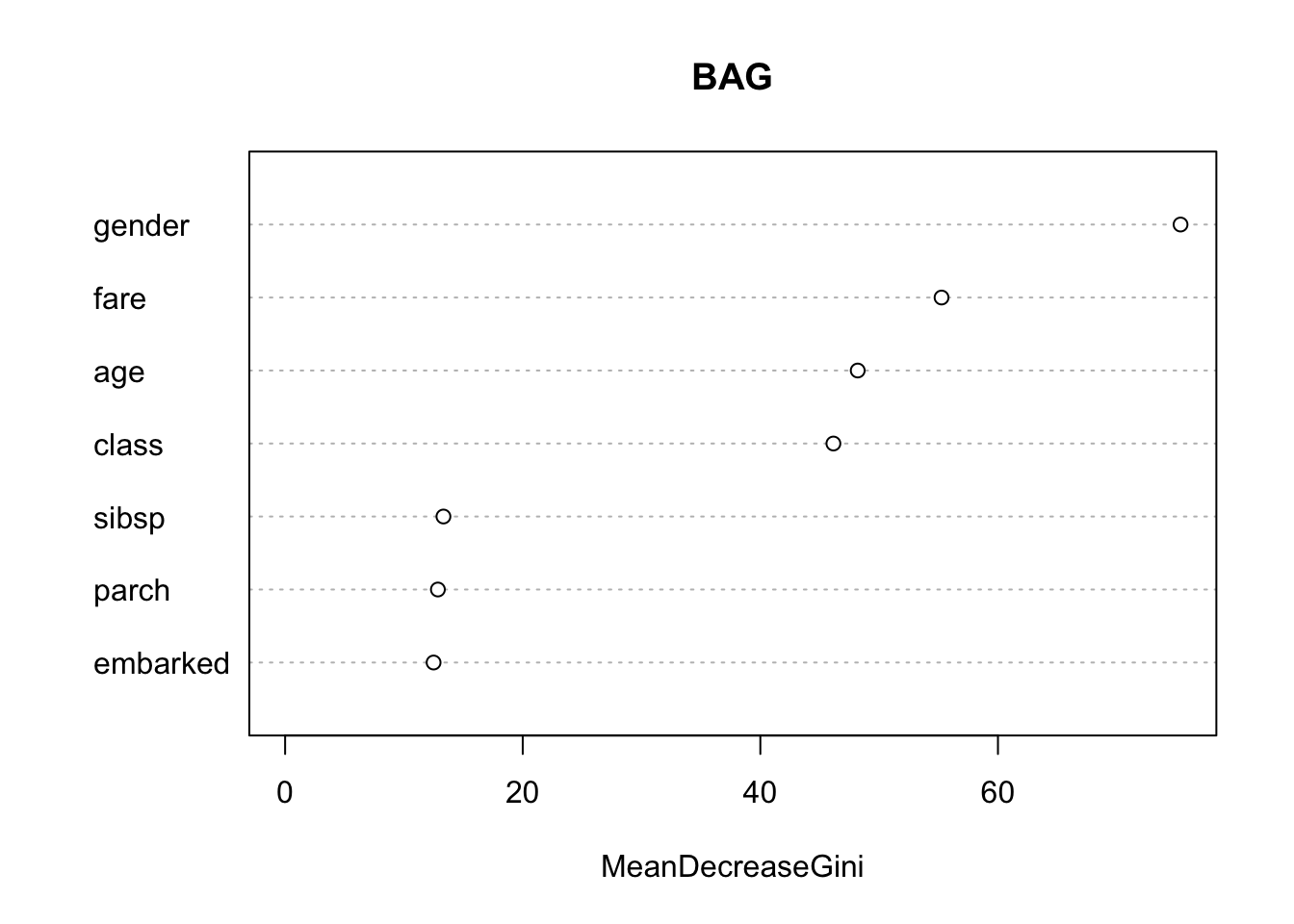
Since we now have 500 trees, many of which are different, how do we interpret the how important individual predictors are to the tree?
We can use the Importance value.
- This is an average of the decrease in Gini Index (classification) or MSE (regression) for each variable across the set of \(B\) trees.
- The larger the number, the more important the variable.
You can access the importance value directly with importance() or plot with varImpPlot().
8.9.2 Evaluating Prediction Accuracy
Random Forest uses all the OOB data to evaluate prediction accuracy.
Each of the \(n\) observations should have an OOB estimate \(\hat{y}_{i_{OOB}}\) constructed as in Equation 8.2. These can used as the predictions to calculate an overall MSEP as follows:
\[MSEP = \frac{1}{n}\sum_i^n(\hat{y}_{i_{OOB}} - y_i)^2 \quad\text{Regression trees}\]
\[\text{Pred Error Rate } = \frac{\sum I(\hat{y}_{i_{OOB}} \neq y_i)}{n}\]
8.9.3 Tuning the Random Forest
We can tune to find the optimal number of trees and the number of variables (\(m\)) used at each split.
- Bagging is an extreme case of Random Forest when \(m = p\).
In a random forest, the algorithm chooses the \(m\) variables at random for each split.
In R, we use arguments ntree and mtry to tune this selection.
Let’s do a quick comparison.
set.seed(123)
BAG <- randomForest(survived ~ gender + age + class + embarked +
fare + sibsp + parch, data = titanicZ[Z,],
mtry = 2)
BAG
Call:
randomForest(formula = survived ~ gender + age + class + embarked + fare + sibsp + parch, data = titanicZ[Z, ], mtry = 2)
Type of random forest: classification
Number of trees: 500
No. of variables tried at each split: 2
OOB estimate of error rate: 21.49%
Confusion matrix:
no yes class.error
no 667 54 0.07489598
yes 180 188 0.48913043set.seed(123)
BAG <- randomForest(survived ~ gender + age + class + embarked +
fare + sibsp + parch, data = titanicZ[Z,],
mtry = 3)
BAG
Call:
randomForest(formula = survived ~ gender + age + class + embarked + fare + sibsp + parch, data = titanicZ[Z, ], mtry = 3)
Type of random forest: classification
Number of trees: 500
No. of variables tried at each split: 3
OOB estimate of error rate: 22.13%
Confusion matrix:
no yes class.error
no 655 66 0.09153953
yes 175 193 0.47554348set.seed(123)
BAG <- randomForest(survived ~ gender + age + class + embarked +
fare + sibsp + parch, data = titanicZ[Z,],
mtry = 4)
BAG
Call:
randomForest(formula = survived ~ gender + age + class + embarked + fare + sibsp + parch, data = titanicZ[Z, ], mtry = 4)
Type of random forest: classification
Number of trees: 500
No. of variables tried at each split: 4
OOB estimate of error rate: 22.31%
Confusion matrix:
no yes class.error
no 654 67 0.09292649
yes 176 192 0.47826087- Here it looks like 2 is better than 3 or 4 on the training data.
For quick tuning to find the optimal \(m\), use tuneRF() to find the optimal value based on OOB error rate.
- Select a training set. Provide the
Xand theYresponse and a starting number of parameters. - It will stop when it reaches the minimum or the max \(m\).
mtry = 2 OOB error = 21.67%
Searching left ...
mtry = 1 OOB error = 22.31%
-0.02966102 0.05
Searching right ...
mtry = 4 OOB error = 22.87%
-0.05508475 0.05 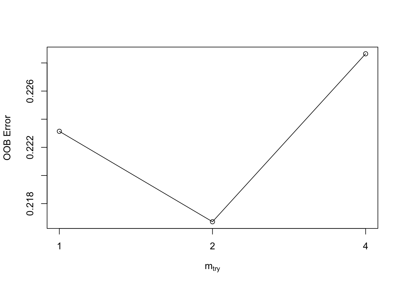
mtry OOBError
1.OOB 1 0.2231405
2.OOB 2 0.2167126
4.OOB 4 0.2286501We can tune both \(m\) and the number of trees as we will see in the next section.
8.9.4 Example of Random Forest with a Regression Tree
Let’s create a regression tree using the Housing data.
homes <- read_csv("https://raw.githubusercontent.com/rressler/data_raw_courses/main/HOME_SALES.csv")
glimpse(homes)
Rows: 522
Columns: 13
$ ID <dbl> 1, 2, 3, 4, 5, 6, 7, 8, 9, 10, 11, 12, 13, 14, 15, 16,…
$ SALES_PRICE <dbl> 360000, 340000, 250000, 205500, 275500, 248000, 229900…
$ FINISHED_AREA <dbl> 3032, 2058, 1780, 1638, 2196, 1966, 2216, 1597, 1622, …
$ BEDROOMS <dbl> 4, 4, 4, 4, 4, 4, 3, 2, 3, 3, 7, 3, 5, 5, 3, 5, 2, 3, …
$ BATHROOMS <dbl> 4, 2, 3, 2, 3, 3, 2, 1, 2, 3, 5, 4, 4, 4, 3, 5, 2, 4, …
$ GARAGE_SIZE <dbl> 2, 2, 2, 2, 2, 5, 2, 1, 2, 1, 2, 3, 3, 2, 2, 2, 2, 2, …
$ YEAR_BUILT <dbl> 1972, 1976, 1980, 1963, 1968, 1972, 1972, 1955, 1975, …
$ STYLE <dbl> 1, 1, 1, 1, 7, 1, 7, 1, 1, 1, 7, 1, 7, 5, 1, 6, 1, 7, …
$ LOT_SIZE <dbl> 22221, 22912, 21345, 17342, 21786, 18902, 18639, 22112…
$ AIR_CONDITIONER <chr> "YES", "YES", "YES", "YES", "YES", "YES", "YES", "YES"…
$ POOL <chr> "NO", "NO", "NO", "NO", "NO", "YES", "NO", "NO", "NO",…
$ QUALITY <chr> "MEDIUM", "MEDIUM", "MEDIUM", "MEDIUM", "MEDIUM", "MED…
$ HIGHWAY <chr> "NO", "NO", "NO", "NO", "NO", "NO", "NO", "NO", "NO", …Let’s create a validation set.
We will ignore ID and predict sales price using the other variables.
Let’s create a random forest using all of the variables and plot it.
Call:
randomForest(formula = SALES_PRICE ~ . - ID, data = homes[Z, ], mtry = 11)
Type of random forest: regression
Number of trees: 500
No. of variables tried at each split: 11
Mean of squared residuals: 3368183142
% Var explained: 81.71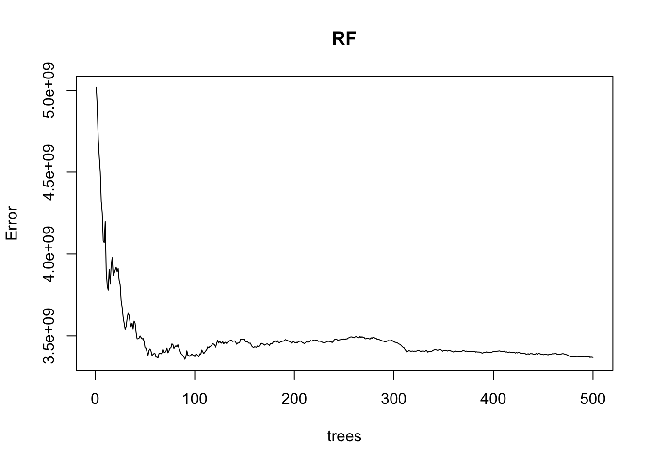
We can find the number of trees that provided the minimum MSE - this is helpful to avoid excessive computations.
[1] 90
Call:
randomForest(formula = SALES_PRICE ~ . - ID, data = homes[Z, ], mtry = 11, ntree = which.min(RF$mse))
Type of random forest: regression
Number of trees: 90
No. of variables tried at each split: 11
Mean of squared residuals: 3452117773
% Var explained: 81.25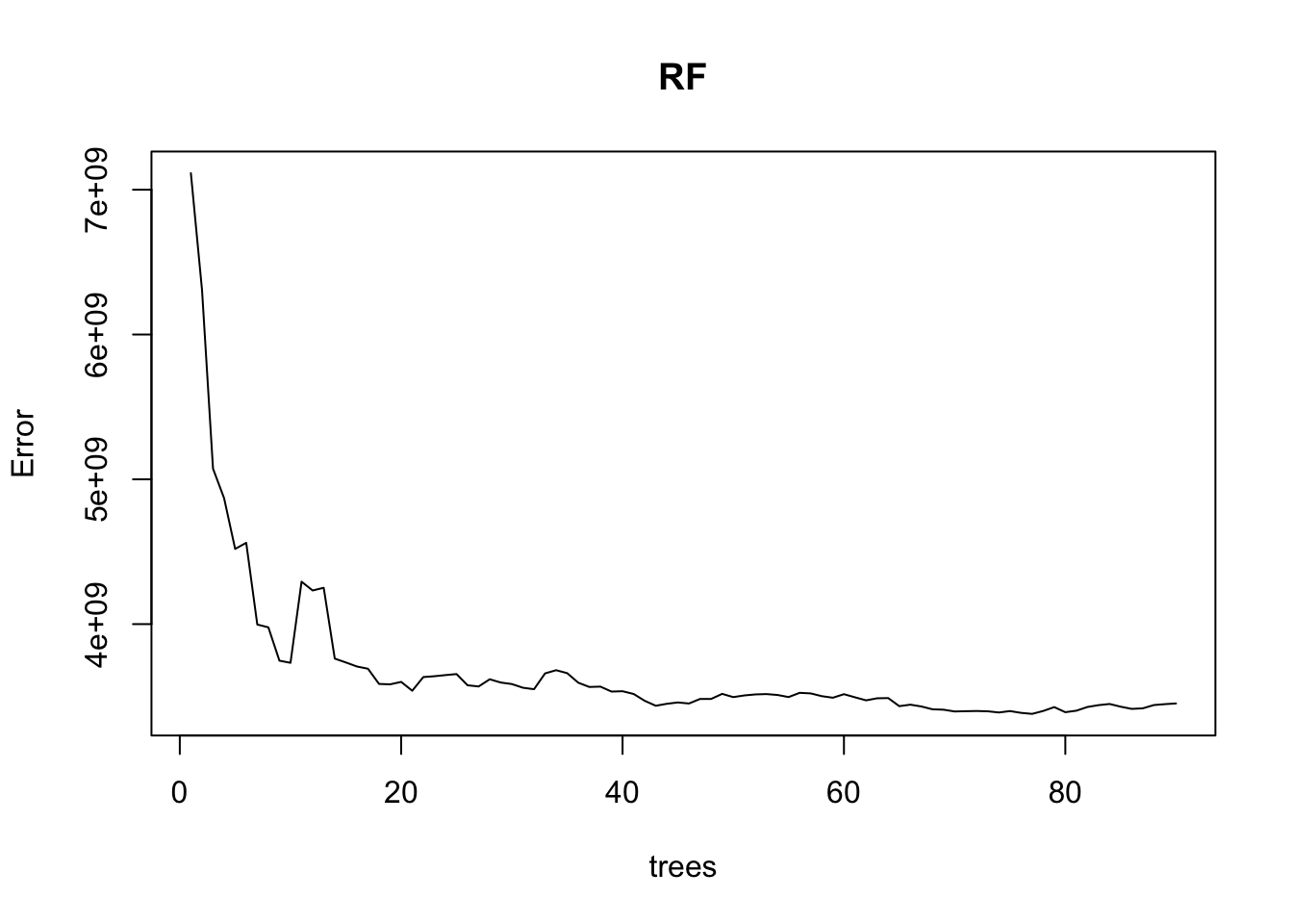
We are using $mse as our performance metric.
Let’s use a for-loop to tune the number of variables \(m\) to select for the splits.
Run the for-loop for each possible value of \(m\) from 1 to \(p\) to get the RMSE.
- Create a random forest and find the optimal number of trees for that \(m\) using the training data.
- Create a random forest with that optimal number of trees using the training data.
- Predict the responses using the trained model with the test data.
- Save the square root of the predicted mean square error.
set.seed(123)
for (k in 1:p) {
RF <- randomForest(SALES_PRICE ~ . -ID, data = homes[Z,], mtry = k)
OptimalTrees[k] <- which.min(RF$mse)
RF <- randomForest(SALES_PRICE ~ . -ID, data = homes[Z,], mtry = k,
ntree = OptimalTrees[k])
Yhat <- predict(RF, newdata = homes[-Z,])
RMSEP[k] <- sqrt(mean((Yhat - homes$SALES_PRICE[-Z])^2) )
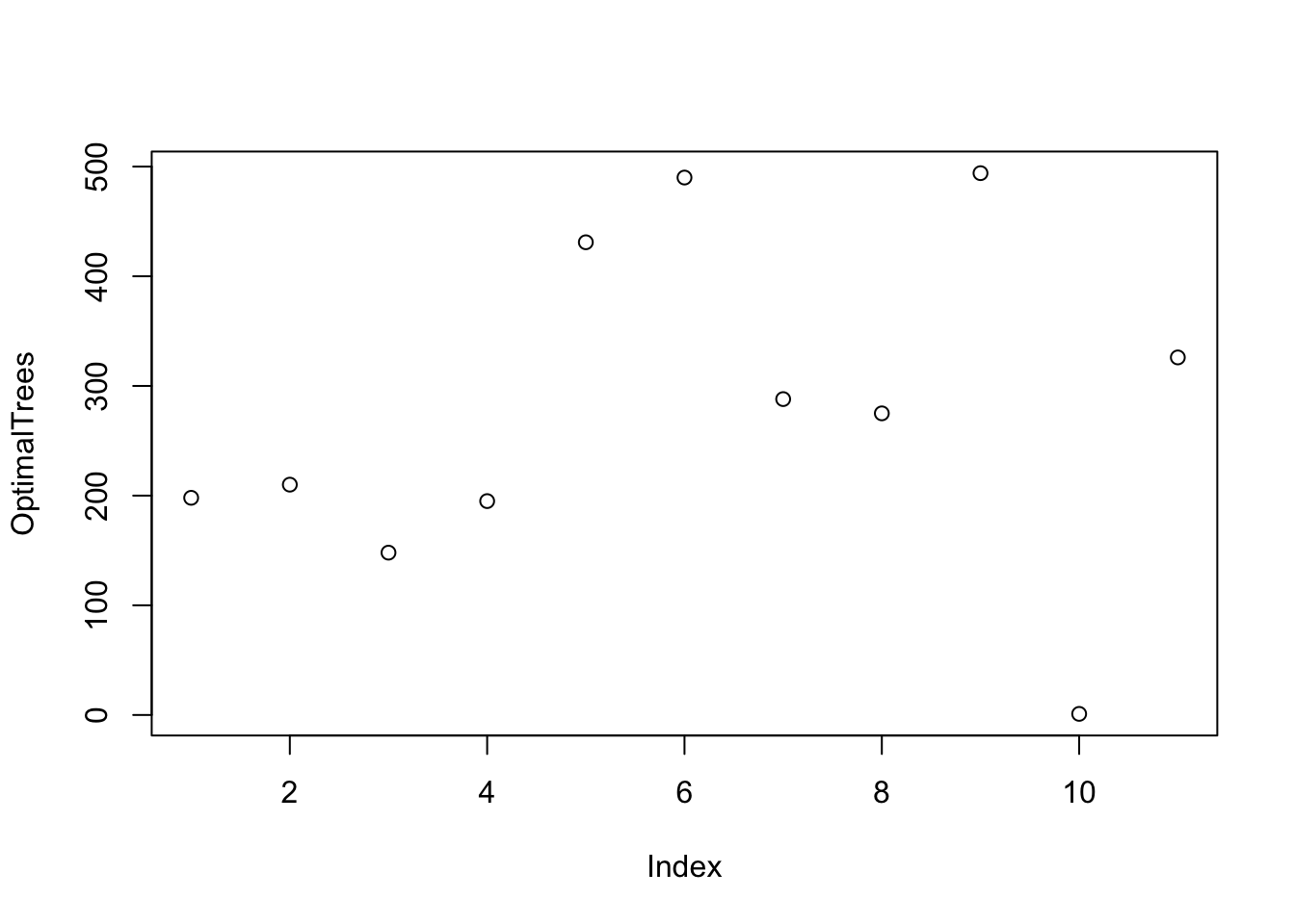
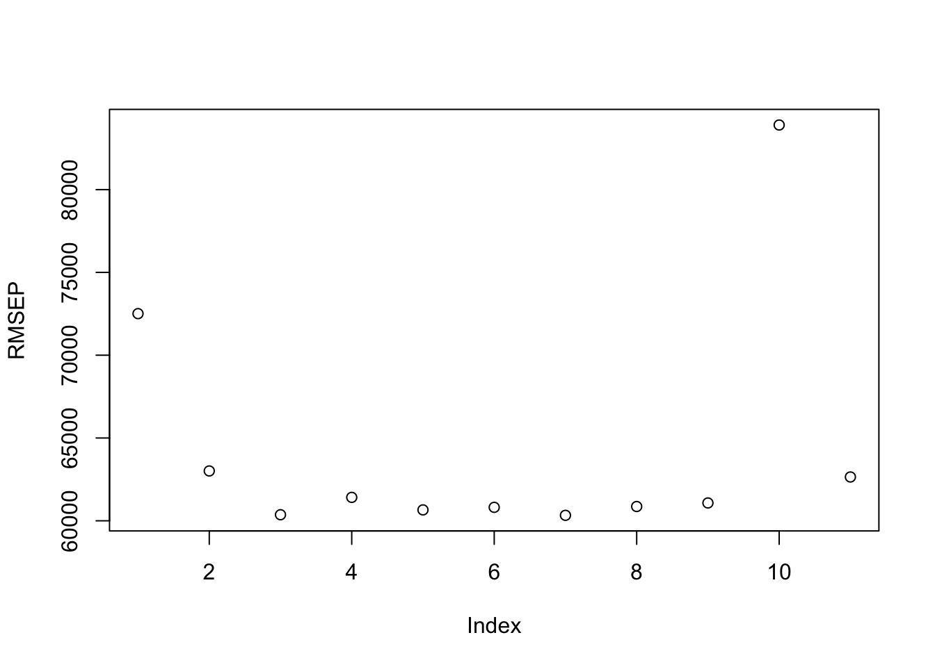
}Now we can plot the optimal Trees for each \(m\) and the RMSE for each \(m\).
Let’s find the best combination of \(m\) and the trees for that \(m\).
So it appears that using \(m = 7\) variables for each split is optimal with 288 trees for this selection.
- A different seed may yield different results. As an example, using 1234 yields \(m\) of 5 with 399 trees and an RMSE of 60,798.55.
8.10 Boosting
In Random Forests we build an ensemble of trees. The trees are constructed independently of each other so we could build each tree in parallel. However, even with limiting the number of variables at each split, Random Forest trees can be susceptible to extreme values.
Boosting is a general method for combining multiple weak predictors to make a stronger predictor through an additive, forward moving process.
Boosting trees is a different approach to building an ensemble of trees. The goal is to reduce the chances of overfitting and build trees in an efficient manner.
When boosting, the trees are grown sequentially so the next tree is grown using information from previously grown trees.
- This is known as sequential learning.
- Since each tree depends on the previous tree, they cannot be built in parallel so it can take longer to run.
Instead of building a large tree based on the original data and then pruning, boosting builds an initial (shallow) tree and then creates additional shallow trees based on the residuals from the previous fitted tree.
Let’s consider a boosted regression tree.
- The original tree is built based on the response values \(y_i\).
- It produces predictions \(\hat{y}_{i1}\).
- The second tree is built using the using the residuals (\(y_i = \hat{y}_{i1)})\) as the response variable in the random forest model.
- The two trees are combined to produce updated (improved) predictions \(\hat{y}_{i2} = \hat{y}_{i1} + \lambda \hat{y}_{i2}\).
- In general, the \(j+1\)th tree is built using the residuals from the previous iteration \((\hat{y}_{ij-1} -\hat{y}_{ij})\) as the response variable in the \(j+1\) random forest model.
- The algorithm stops when the chosen number of trees \(B\) has been built to create the entire ensemble.
Each new tree should be small so instead of creating one large tree, we are creating a lot of small trees, each trying to explain the remaining unexplained variance.
- It is a stage-wise (not step-wise) process as the new tree is used with the unchanged previous trees to generate updated predictions \(\hat{y}_{ij}\).
- This ensemble of week trees can produce strong results when generated and combined in this way.
Boosting also works on classification trees but the approach is slightly different.
Boosting can also incorporate the random forest selection of variables to be considered for each new tree.
Boosting can work for multiple distributions to describe the loss function being optimized. These include Gaussian (regression, MSE) and Bernoulli (Classification, Error rate).
Consider Boosting as a method of descending the gradient of the tree in small steps by weighting the residuals from the previous step so the larger residuals influence the next tree more heavily to fit them better.
8.10.1 Boosting works with three main tuning parameters
-
\(B\): the number of trees to be built for the ensemble.
- While this can be in the hundreds or hundreds of thousands, the algorithm tends to overfit if \(B\) gets too large.
- You can use cross validation to select \(B\).
-
\(d\): the number of splits to use in each new tree.
- Typically \(d\) is small, 1 or 2, so the trees learn slowly to reduce overfitting.
- This is also known as the interaction depth.
- You get trees with \(d+1\) terminal nodes.
-
\(\lambda\): the shrinkage parameter or the learning parameter.
- This controls how much change can occur in a tree based on the shrinking the effects of the new tree on the prediction and thus the residuals.
- You can also think of it as the shrinking the step size taken when moving along the gradient descent.
- Typically \(\lambda\) is small, such as .01 or .001 and the smaller the \(\lambda\) the better the performance.
- However, very small \(\lambda\) will increase run time as they usually require more trees, larger \(B\), to get good results.
By selecting these parameters to optimize “slow learning”, an ensemble (series), of many weakly performing trees can be combined to create an effective predictor with low risk of overfitting.
8.10.2 Example of Boosting in R
We will use the {gbm} package.
Let’s use the home sales data.
We need to convert each character variable to a factor to use it in the model.
Rows: 522
Columns: 13
$ ID              <dbl> 1, 2, 3, 4, 5, 6, 7, 8, 9, 10, 11, 12, 13, 14, 15, 16,…
$ SALES_PRICE     <dbl> 360000, 340000, 250000, 205500, 275500, 248000, 229900…
$ FINISHED_AREA   <dbl> 3032, 2058, 1780, 1638, 2196, 1966, 2216, 1597, 1622, …
$ BEDROOMS        <dbl> 4, 4, 4, 4, 4, 4, 3, 2, 3, 3, 7, 3, 5, 5, 3, 5, 2, 3, …
$ BATHROOMS       <dbl> 4, 2, 3, 2, 3, 3, 2, 1, 2, 3, 5, 4, 4, 4, 3, 5, 2, 4, …
$ GARAGE_SIZE     <dbl> 2, 2, 2, 2, 2, 5, 2, 1, 2, 1, 2, 3, 3, 2, 2, 2, 2, 2, …
$ YEAR_BUILT      <dbl> 1972, 1976, 1980, 1963, 1968, 1972, 1972, 1955, 1975, …
$ STYLE           <dbl> 1, 1, 1, 1, 7, 1, 7, 1, 1, 1, 7, 1, 7, 5, 1, 6, 1, 7, …
$ LOT_SIZE        <dbl> 22221, 22912, 21345, 17342, 21786, 18902, 18639, 22112…
$ AIR_CONDITIONER <chr> "YES", "YES", "YES", "YES", "YES", "YES", "YES", "YES"…
$ POOL            <chr> "NO", "NO", "NO", "NO", "NO", "YES", "NO", "NO", "NO",…
$ QUALITY         <chr> "MEDIUM", "MEDIUM", "MEDIUM", "MEDIUM", "MEDIUM", "MED…
$ HIGHWAY <chr> "NO", "NO", "NO", "NO", "NO", "NO", "NO", "NO", "NO", …8.10.2.1 Building the Boosted Ensemble
Now we can build the model with the training data and see the summary.
- Set
n.trees=5000to start instead of the default 100. - the default
disinteraction.depth=1. - The default \(\lambda\) is
shrinkage=0.1. - Set
distribution ="gaussian"since we are doing least squares regression. - The output is a
gbm.object. See?gbm.objectfor details. - Then check the
summary()(?summary.gbm) to see the relative influence of each variable in the ensemble model normalized to 100.- For
distribution="gaussian"this returns exactly the reduction of squared error attributable to each variable. - Note: the code is in the
print.gbm.Rfunction and you cannot adjust the barplot attributes.
- For
set.seed(123)
Z <- sample(nrow(homes), nrow(homes)/2)
set.seed(123)
boosth <- gbm(SALES_PRICE ~ . - ID, data = homes[Z,],
n.trees = 5000, distribution = "gaussian")
boosthgbm(formula = SALES_PRICE ~ . - ID, distribution = "gaussian",
data = homes[Z, ], n.trees = 5000)
A gradient boosted model with gaussian loss function.
5000 iterations were performed.
There were 11 predictors of which 10 had non-zero influence.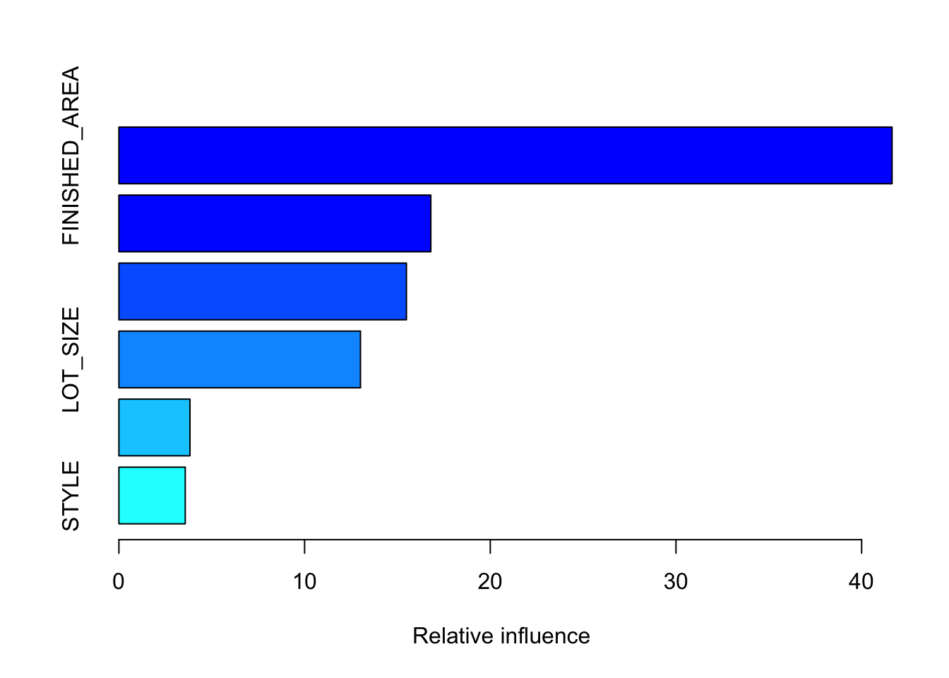
                            var    rel.inf
FINISHED_AREA     FINISHED_AREA 41.6378622
YEAR_BUILT           YEAR_BUILT 16.7978453
QUALITY                 QUALITY 15.4843121
LOT_SIZE               LOT_SIZE 13.0096535
BEDROOMS               BEDROOMS  3.8274367
STYLE                     STYLE  3.5735513
BATHROOMS             BATHROOMS  3.4374819
GARAGE_SIZE         GARAGE_SIZE  1.5708073
POOL                       POOL  0.4075263
AIR_CONDITIONER AIR_CONDITIONER  0.2535233
HIGHWAY                 HIGHWAY  0.0000000
To see a given tree structure use pretty.gbm.tree(object, i.tree= j) where j is the number of the tree.
- This is not necessary for the analysis but can help to understand what the individual “weak” trees might look like.
  SplitVar SplitCodePred LeftNode RightNode MissingNode ErrorReduction Weight
0        0     2613.5000        1         2           3   1.502409e+12    130
1       -1    -6567.2724       -1        -1          -1   0.000000e+00     92
2       -1    17069.0592       -1        -1          -1   0.000000e+00     38
3       -1      341.8091       -1        -1          -1   0.000000e+00    130
  Prediction
0   341.8091
1 -6567.2724
2 17069.0592
3 341.8091 SplitVar SplitCodePred LeftNode RightNode MissingNode ErrorReduction Weight
0 6 22013.50000 1 2 3 2637144773 130
1 -1 -588.11907 -1 -1 -1 0 57
2 -1 319.57564 -1 -1 -1 0 73
3 -1 -78.41358 -1 -1 -1 0 130
Prediction
0 -78.41358
1 -588.11907
2 319.57564
3 -78.41358The output is a data frame where each row is a node in the tree.
- The left column is the node number with the root being 0.
- Note:
gbm()uses a c++ engine for the boosting which returns variable indices starting with 0 so add 1 to get the variable.
- Note:
-
SplitVar: the index of which variable is split. The -1 indicates a terminal or leaf node. -
SplitCodePred: If the split variable is continuous this is the split point. If it’s categorical is the index of object$c.split that describes the categorical split. If the node is a terminal node ,this is the prediction. - The prediction is weighted by the learning rate.
- The last row is the node to use if there is an
NAin the data (as indicated by the index in theMissingNodevariable for the root node). That is why there are three leaf nodes for a binary tree with one split.
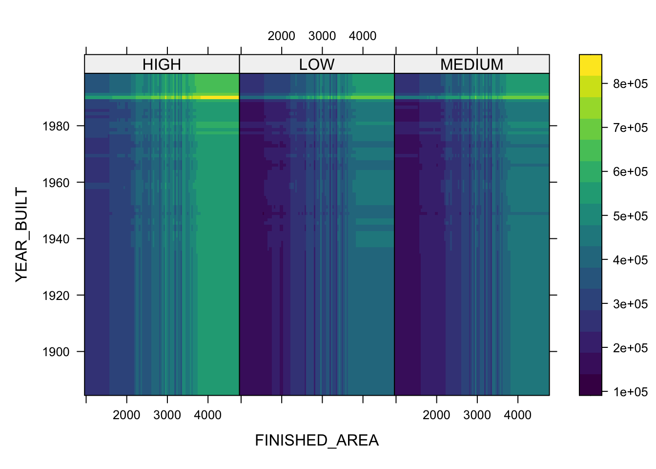
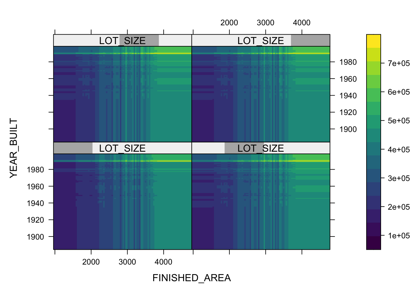
Partial variable plots show the marginal effect of individual variables on the response variable ( here \(Y\) is SALES_PRICE) after all others are accounted for. (?plot.gbm)
- Let’s look at the top three.
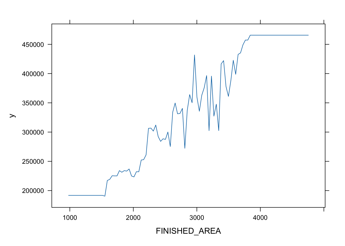
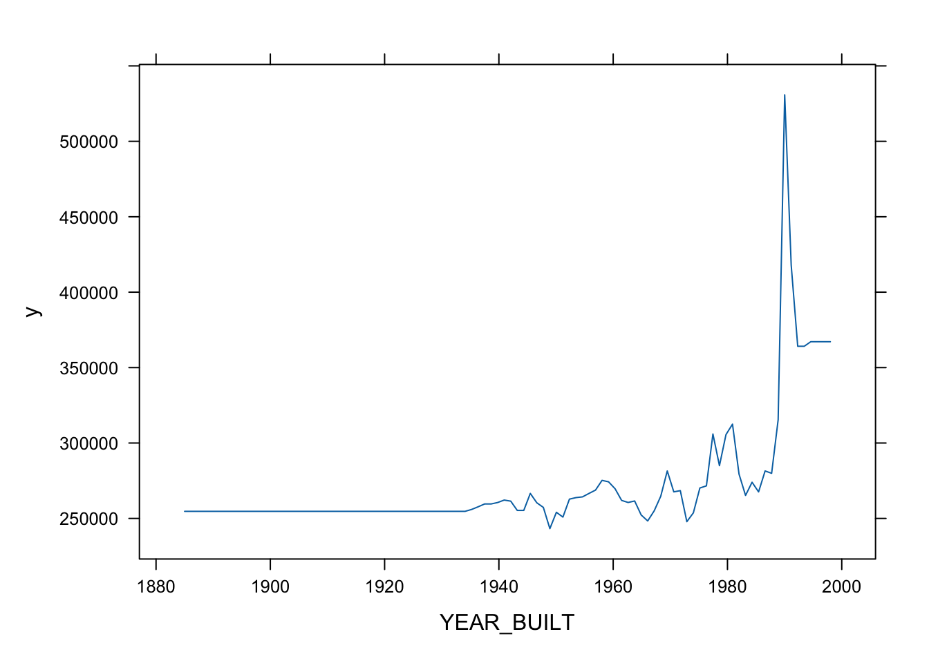
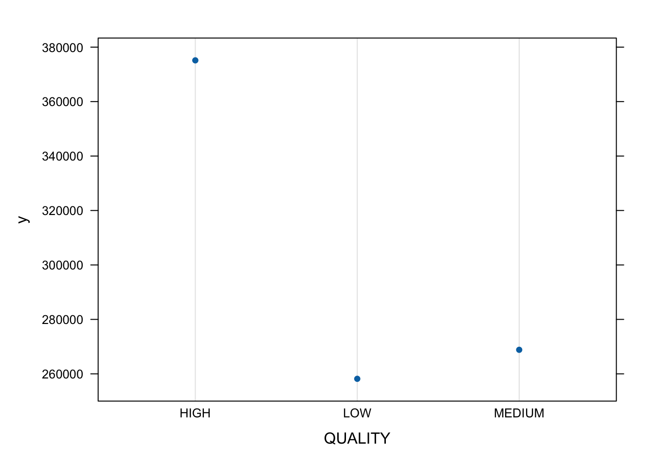
- You can also plot two or three variables to get a contour plot.
plot(boosth, c("FINISHED_AREA", "YEAR_BUILT"))
plot(boosth, c("FINISHED_AREA", "YEAR_BUILT", "QUALITY"))
plot(boosth, c("FINISHED_AREA", "YEAR_BUILT", "LOT_SIZE"))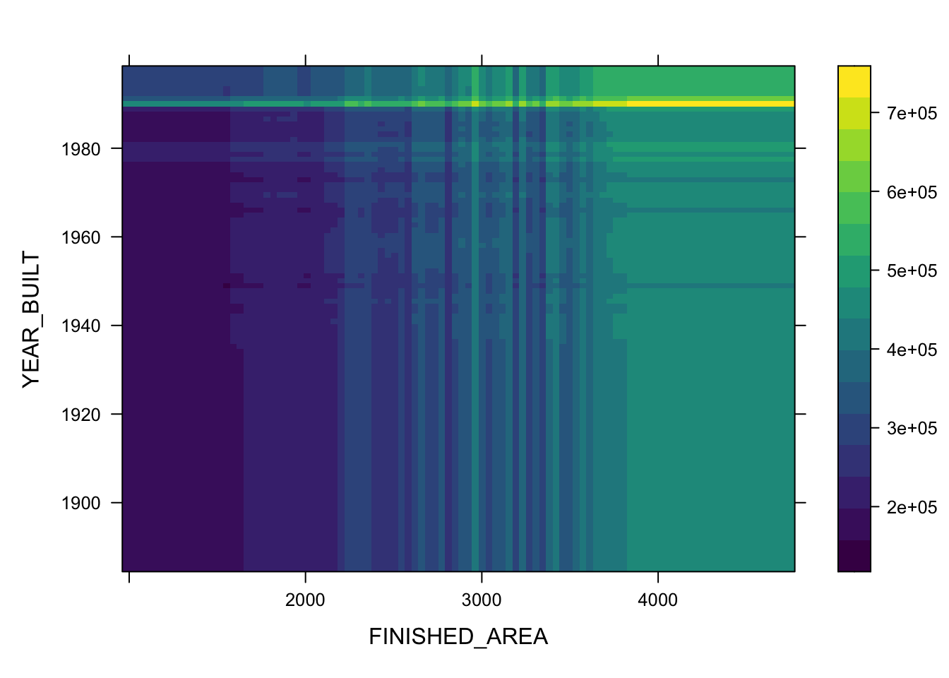
8.10.3 Prediction
Let’s predict.
?predict.gbm- If doing for classification with
distribution="bernoulli", usetype="response"to get the predictions in the levels ofY, instead of the log-odds.
Yhat <- predict(boosth, newdata = homes[-Z,], n.trees = 5000)
mean((Yhat - homes$SALES_PRICE[-Z])^2)^.5
[1] 67482.13Let’s adjust the shrinkage parameter.
set.seed(123)
boosth <- gbm(SALES_PRICE ~ . - ID, data = homes[Z,],
              n.trees = 5000, shrinkage = .001,
              distribution = "gaussian")
summary(boosth)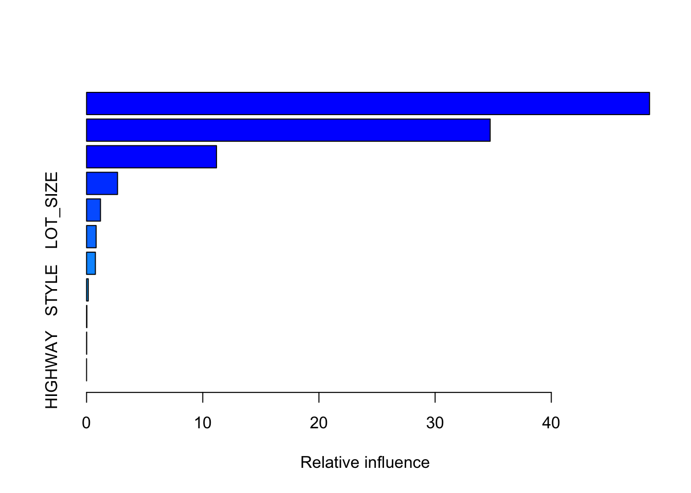
                            var     rel.inf
FINISHED_AREA     FINISHED_AREA 48.45477129
QUALITY                 QUALITY 34.73763114
YEAR_BUILT           YEAR_BUILT 11.18296508
BATHROOMS             BATHROOMS  2.66518029
LOT_SIZE               LOT_SIZE  1.19705485
BEDROOMS               BEDROOMS  0.82130716
GARAGE_SIZE         GARAGE_SIZE  0.75844367
STYLE                     STYLE  0.14509256
AIR_CONDITIONER AIR_CONDITIONER  0.02671275
POOL                       POOL  0.01084121
HIGHWAY                 HIGHWAY  0.00000000
Yhat <- predict(boosth, newdata = homes[-Z,], n.trees = 5000)
mean((Yhat - homes$SALES_PRICE[-Z])^2)^.5[1] 62831.67So reducing the shrinkage rate in this case improved the prediction RMSE.
8.10.3.1 Cross Validation for the Number of Trees
We can change the cv.folds= parameter to have it use cross validation for the number of trees.
- Set the number high.
set.seed(123)
boosth <- gbm(SALES_PRICE ~ . - ID, data = homes[Z,],
              n.trees = 30000, shrinkage = .001,
              cv.folds = 10,
              distribution = "gaussian")
boosth
gbm(formula = SALES_PRICE ~ . - ID, distribution = "gaussian",
data = homes[Z, ], n.trees = 30000, shrinkage = 0.001, cv.folds = 10)
A gradient boosted model with gaussian loss function.
30000 iterations were performed.
The best cross-validation iteration was 22198.
There were 11 predictors of which 10 had non-zero influence.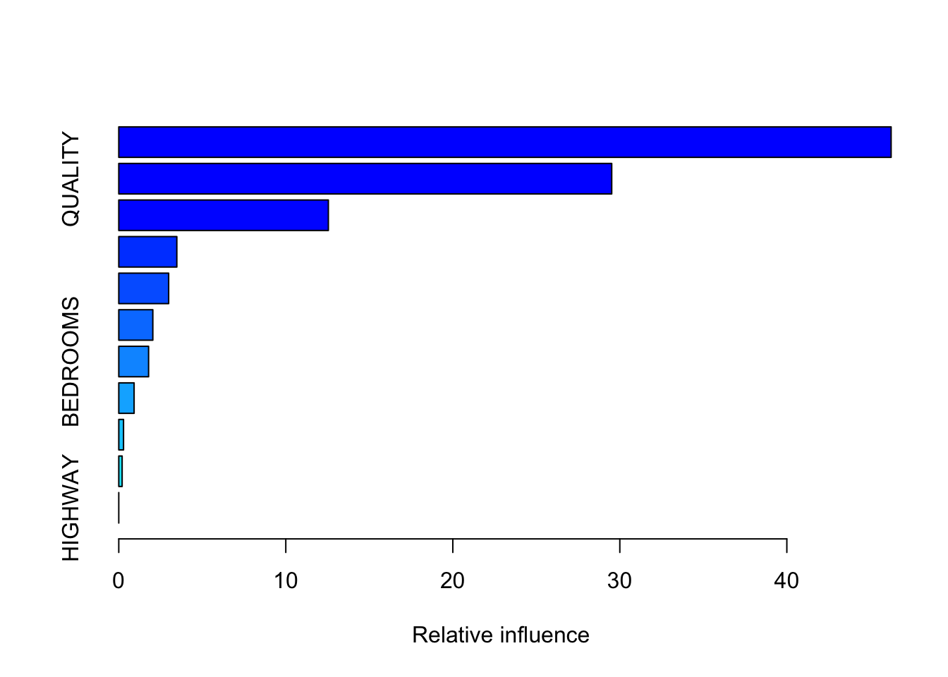
                            var    rel.inf
FINISHED_AREA     FINISHED_AREA 46.2432052
QUALITY                 QUALITY 29.5149635
YEAR_BUILT           YEAR_BUILT 12.5490853
LOT_SIZE               LOT_SIZE  3.4763711
BATHROOMS             BATHROOMS  2.9872416
STYLE                     STYLE  2.0391167
BEDROOMS               BEDROOMS  1.7853434
GARAGE_SIZE         GARAGE_SIZE  0.9182208
POOL                       POOL  0.2849619
AIR_CONDITIONER AIR_CONDITIONER  0.2014905
HIGHWAY                 HIGHWAY  0.0000000
The output object now includes a vector of the cross validated error rate (cv.error) for each tree.
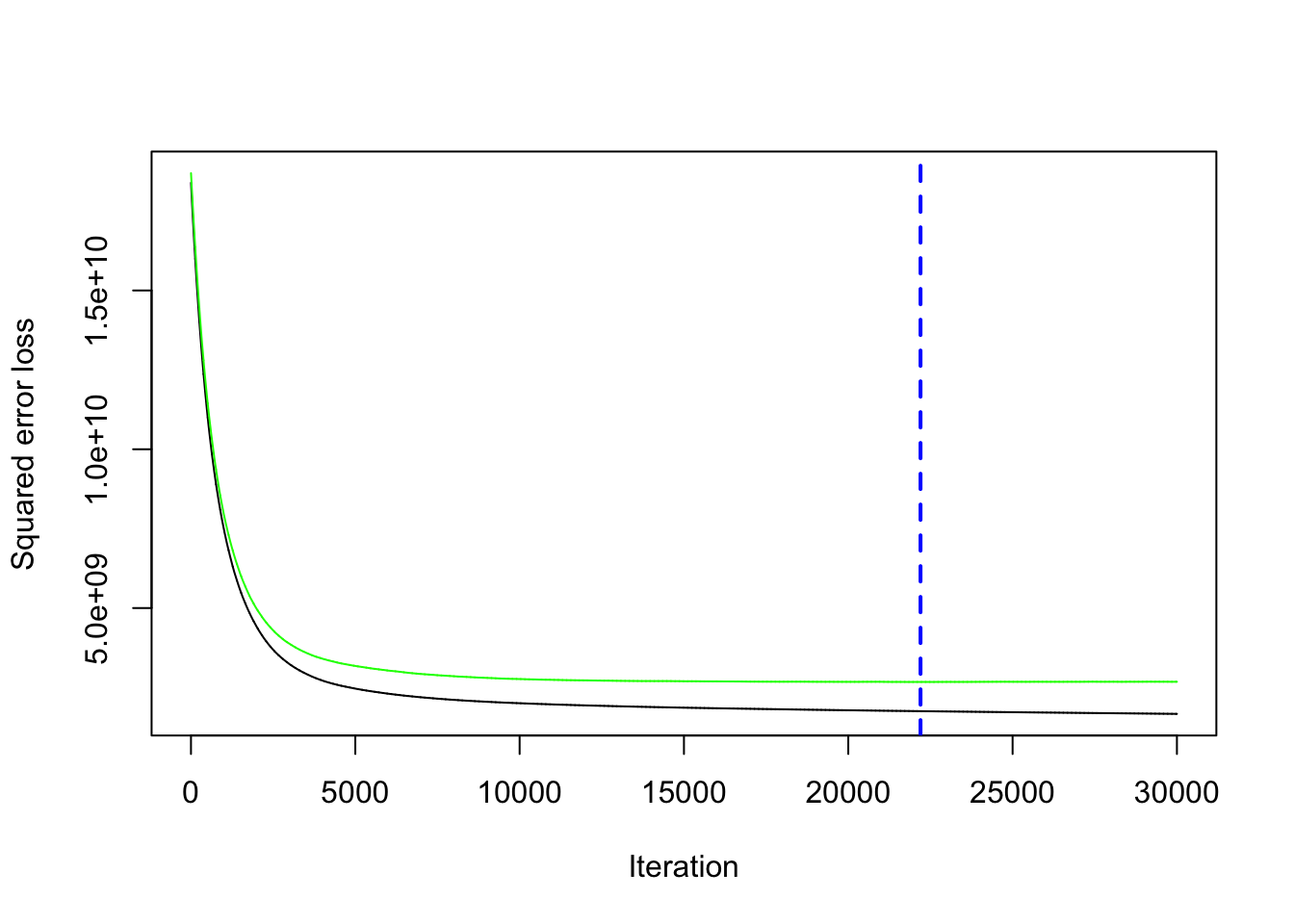
- You can plot the performance for the number of trees with
gbm.perf(). - The black line is the training deviance and the green line is the testing deviance.
- The tree selected for prediction, indicated by the vertical blue line, is the tree that minimizes the testing error on the cross-validation folds.
- The smaller you set
shrinkage=the more trees you will need.
Now you can predict on the testing data to calculate MSEP.
- It will use the optimal number of trees from the output if you used
cv.foldsgreater than 1.
[1] 61032.52In this case, Random Forests still did better at 60330.43.
You can experiment by making the shrinkage parameter smaller to see how many trees it uses and if it does better on prediction.
Trees provide a relatively explainable approach to regression and classification models.
Trees have a tendency to overfit thus careful pruning or use of Bagging, Random Forests, and Boosting are important methods in developing more accurate and useful models.
