5  Cross-Validation Methods

ISLRv2 Chapter 5 and Handouts

Author

Affiliation

Richard Ressler

American University

5.1 Cross-Validation Methods

Cross-validation is a method for evaluating prediction performance in SML algorithms.

5.1.1 Resampling

Recall, if we used training data to evaluate prediction performance, we would overestimate the true performance on new data due to inevitable over-fitting.

To evaluate prediction accuracy, we have separated our data in training and testing subsets.

This is a type of Resampling as we are drawing samples from the original data set.

There are different methods of Resampling. We have been using the validation set method.

1. Validation Set Method: Split the data into two distinct subsets for training and testing.

• The training set is used for fitting models, tuning, testing significance, selecting predictors, etc.
• The testing data is used only for prediction and performance evaluation.

We have used two of many possible Measures of Performance:

• Prediction MSE in regression problems, and
• Prediction error rate in classification problems.

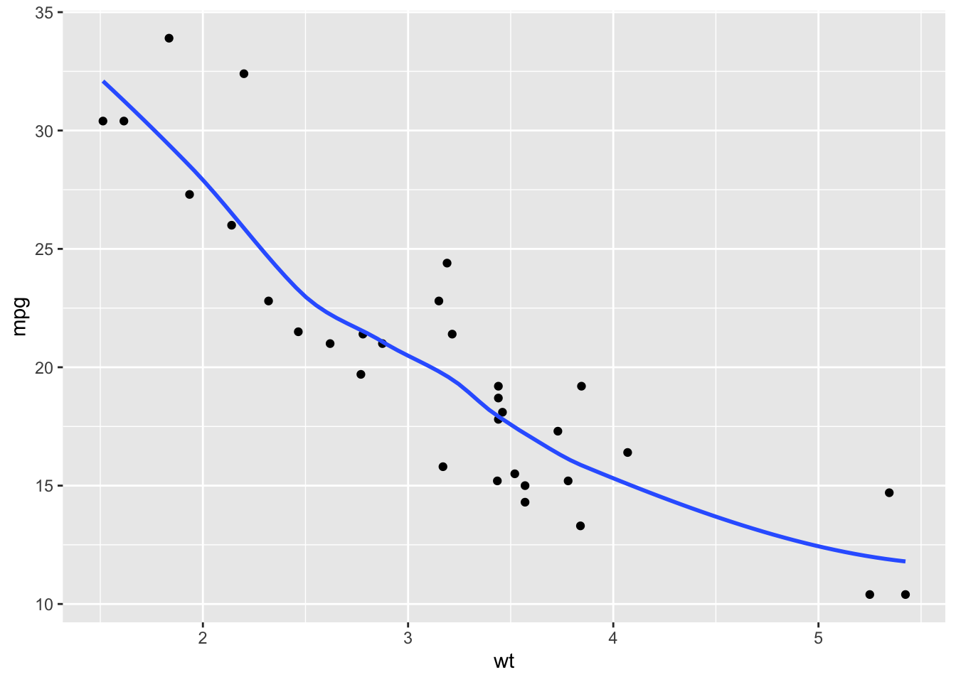
5.1.2 Example of Cross Validation with mtcars Data in R

Let’s plot the data

suppressMessages(library(tidyverse))

ggplot(mtcars, aes(wt, mpg)) +
  geom_point() +
  geom_smooth(se = FALSE)

We can see some non-linearity but perhaps that is just noise. Can we do better with a polynomial model?

We want to know what degree polynomial might be best for predicting the miles per gallon based on the weight of a new car.

We can use a for-loop to fit a series of polynomial regression models using the validation set method.

• Set the seed for the random number generator.
• Break out the training and testing validation sets based on a random sample of the data.
• Use the for loop to create a sequence of polynomial models of degree \(k\) where \(k\) ranges from 1 to 10.
• Fit the model using the training data and predict \(\hat{y}_{i}\) using the test data.
• Calculate the Root Mean Squared Error for each model.

  • Recall, RMSE is the square root of the MSE which is \(\text{SSE}/n\).

  • It is more interpretable at times than MSE since it is in the un-squared units of the original \(Y\), e.g., mpg instead of mpg².

set.seed(1234)
n <- nrow(mtcars)
Z <- sample(n, floor(n/2)) # setting up our re-sample

rmse <- vector(mode = "double", length = 10)
for (k  in seq_along(rmse)) {
  reg <- lm(mpg ~ poly(wt, k), data = mtcars, subset = Z) # training data
  Yhat <- predict(reg, newdata = mtcars[-Z,]) # test data
  Ytest = mtcars$mpg[-Z] # test data
  rmse[[k]] <- sqrt(mean(Yhat - Ytest)^2)
}

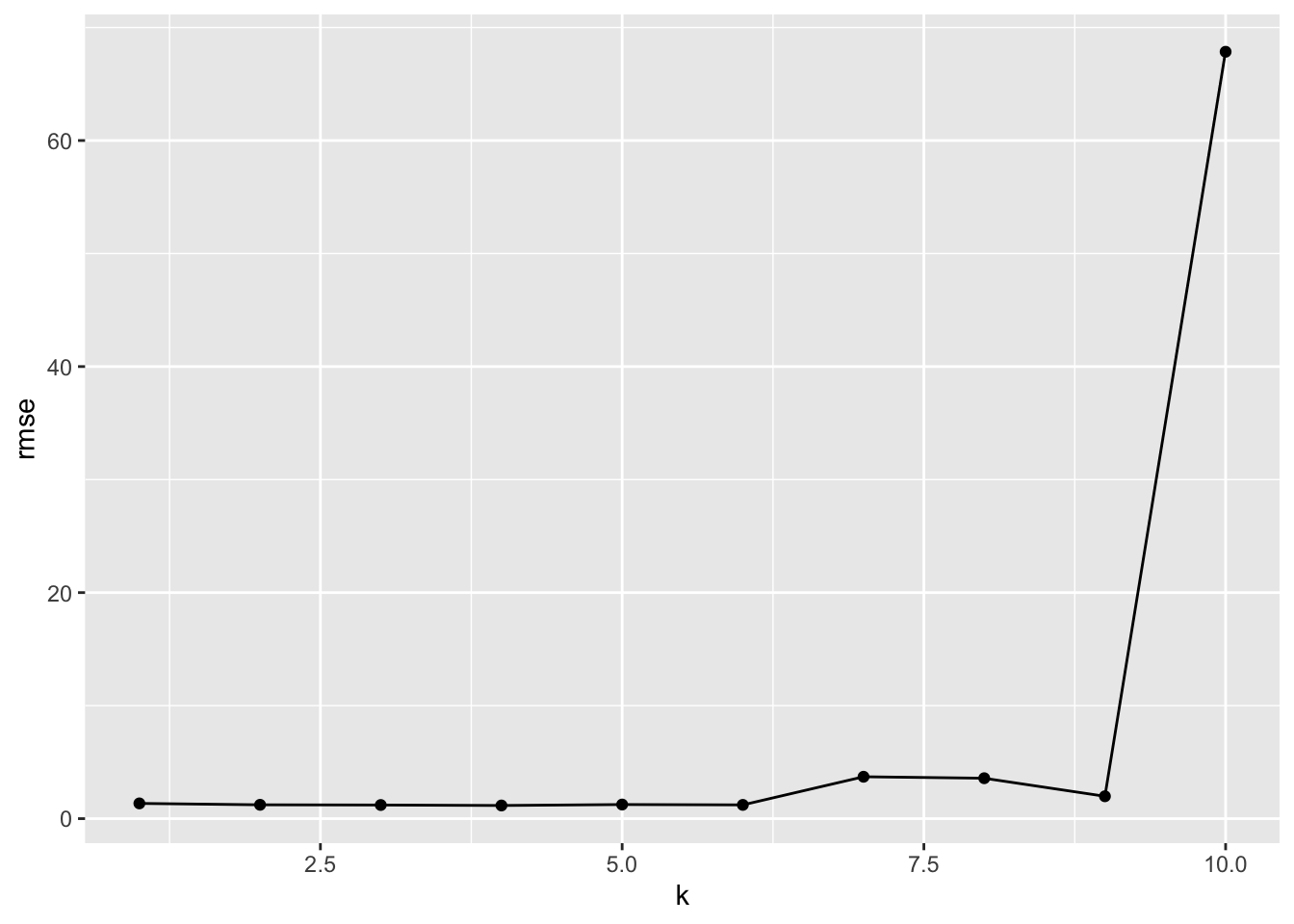
Let’s plot the RMSE versus \(k\) the degree of the polynomial.

ggplot(tibble(k = 1:10, rmse), aes(k, rmse)) +
  geom_point() +
  geom_line()

which.min(rmse)

[1] 4

min(rmse)

[1] 1.164305

• We can see the 10th degree polynomial is way off.

Let’s look at the fitted values for miles per gallon. What do you notice?

Yhat

        Mazda RX4        Datsun 710         Merc 240D          Merc 280 
        33.906610        168.235814         21.948461         17.313192 
        Merc 280C        Merc 450SL       Merc 450SLC Chrysler Imperial 
        17.313192          6.677194          3.065900       -490.900328 
         Fiat 128       Honda Civic    Toyota Corolla     Toyota Corona 
       232.388456       -821.758470       -277.777982         84.806589 
       Camaro Z28  Pontiac Firebird     Porsche 914-2    Ford Pantera L 
        -1.181190         -1.495726        244.371357         22.325850 

Let’s plot the fitted values against the training data and then the test data.

df <- tibble(wt_train = mtcars$wt[Z], 
             mpg_train =  mtcars$mpg[Z],
             Yhat_10 = Yhat)
ggplot(df, aes(wt_train, Yhat_10)) +
  geom_point(color = "purple") +
  geom_smooth(se = FALSE) +
  geom_point(mapping = aes(wt_train, mpg_train), color = "green") +
  ggtitle("Fitted values from the 10 degreee Polynomial on 16 Training Points")
df <- tibble(wt_test = mtcars$wt[-Z], 
             mpg_test =  mtcars$mpg[-Z],
             Yhat_10 = Yhat)
ggplot(df, aes(wt_test, Yhat_10)) +
  geom_point(color = "red") +
  geom_smooth(se = FALSE) +
  geom_point(aes(wt_test, mpg_test)) +
  ggtitle("Predicted values from the 10 degreee Polynomial on 16 Test Points")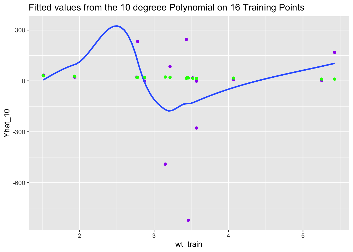

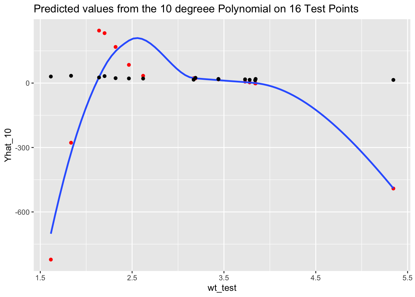
The over-fitting to noise in the training data resulted in predictions that were way off, especially in the values on either end, and thus the large RMSE for the 10th degree polynomial.

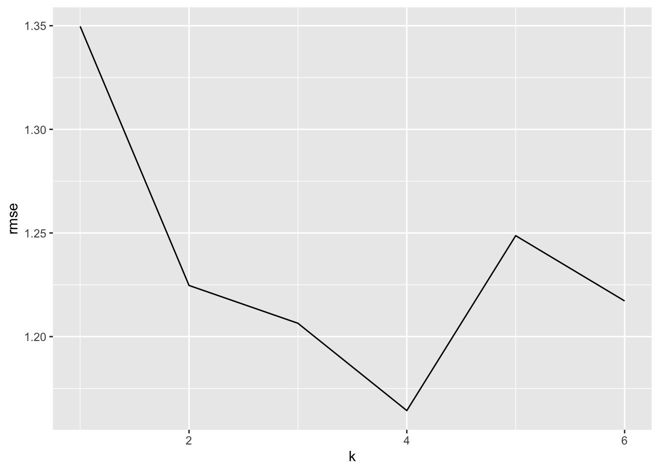
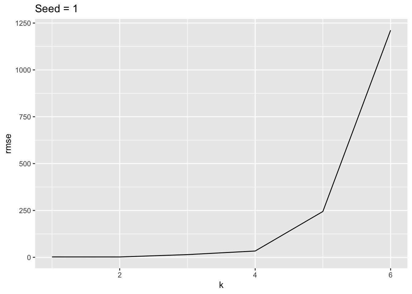
What if we plot the RMSE for the first six polynomials to better see their relative performance?

ggplot(tibble(k = 1:6, rmse = rmse[1:6]), aes(k, rmse)) +
  geom_line()

For this validation set, the 4^th degree was best.

If we used a different seed to create a different split, it could be different.

set.seed(seed <- 1)
n <- nrow(mtcars)
Z <- sample(n, floor(n/2))

rmse <- vector(mode = "double", length = 10)
for (k  in seq_along(rmse)) {
  reg <- lm(mpg ~ poly(wt, k), data = mtcars, subset = Z)
  Yhat <- predict(reg, newdata = mtcars[-Z,])
  Ytest = mtcars$mpg[-Z]
  rmse[[k]] <- sqrt(mean(Yhat - Ytest)^2)
}
which.min(rmse)

[1] 2

min(rmse)

[1] 1.885572

Now the 2^nd degree polynomial is best. This is a small data set so it is not unexpected to see these changes.

ggplot(tibble(k = 1:6, rmse = rmse[1:6]), aes(k, rmse)) +
  geom_line() +
  ggtitle(glue::glue("Seed = {seed}"))

Note

• The above is a basic validation approach called th holdout method that splits that data into two sets: train and test.
• There is another option that is now more popular.
• Split the data into train and test sets and then split the train data set into two sets for model training and model tuning.
• The Model “Training” set is used to create the model, e.g. fitting the model parameters (weights in a neural network, coefficients in regression, etc.).
• The Model “Tuning” set is also called a “validation set”.
  • It is data not used to create the model but to tune the model hyper parameters, e.g., selecting the threshold in Logistics Regression, learning rates, or regularization strength).
  • This helps reduce the risk of overfitting because the model is not directly trained on this set.
  • The purpose is to provide another approach to reducing the chance of overfitting (or “overtuning”) the model to one set of data.
• The model “Test” set is then used to evaluate performance on unseen data as before.
  • This is useful for comparing models against a standard or other models.
• Splitting the data into three sets means choosing what percentage of the data should go into which set.
• Common approaches are to split 60-20-20 or 80-10-10 for really large data sets.
• However, the choice of split depends on the size of the dataset and the task. For smaller datasets, cross-validation (e.g., k-fold cross-validation) is often preferred to make the most out of available data.

Caution

Just because the predictions are off, does not mean people won’t use them.

• See Women ‘may outsprint men by 2156’ based on a 2004 short paper by Tatem et al: Momentous sprint at the 2156 Olympics?.
• What do you notice about the plot?

Figure 1 from Tatem et al, Nature, 431, page525 (2004)

5.2 “Leave-one-out” Cross-Validation (LOOCV)

As seen in previous example, the validation set technique uses only a portion of the data to fit the models.

• We would expect better performance if we used the entire data set for learning and then predicted on some other data.
• In reality though, we don’t usually don’t have other data.
• If we increased the percentage of our data set used for training, we would expect a better fit to the training data.
• But then we have a smaller test sample for estimating \(\text{MSE} = E(\hat{y}_i - y_i)^2\) as

\[ \widehat{\text{MSE}} = \frac{1}{n_{test}}\sum_{i \in test}(\hat{y}_i - y_i)^2 \]

• This suggests our \(\widehat{\text{MSE}}\) will be unreliable and our performance evaluation will not be accurate.

This need to balance the split between training and testing data is the main disadvantage of the validation set method.

We lose a lot of information regardless of what we do.

Leave-one-out cross-validation (aka LOOCV, Jackknife) was developed by British statistician Maurice Quenouille in 1949 (he was 25 years old) and he refined it several years later.

• American statistician John Tukey (of FFT and Box Plot fame) proposed the name “jackknife” as the method is a handy tool for many kinds of problems.

Leave-one-out cross-validation tries to use almost as much data as possible to train the model.

• Use \((n-1)\) points for training and the remaining \(n^{th}\) point for testing.

• This gives almost maximum performance in fitting the model.

• This is denoted as predict 1 response \(y_i\) with \(\hat{y}_{i(-i)}\) where the subscript \((-i)\) means the value \(\hat{y}_{i}\) was predicted based on a model trained without the \(i^{th}\) values of \(Y\) and \(X\) in the training data.

By itself, this is an unreliable estimate. But, we will repeat the same procedure for every data point and generate \(n\) predictions.

Then we have

\[ \widehat{\text{MSE}}_\text{jackknife} = \frac{1}{n}\sum_i^n(\hat{y}_{i(-i)} - y_i)^2 \]

5.2.1 Example of Leave-one-out Cross-Validation in R

Let’s repeat with mtcars for mpg.

• Now the for-loop has loop for each \(k\) and inside that there is the LOOCV for-loop.
  • We leave out the \(i\)th value in each step, fitting the model with lm().
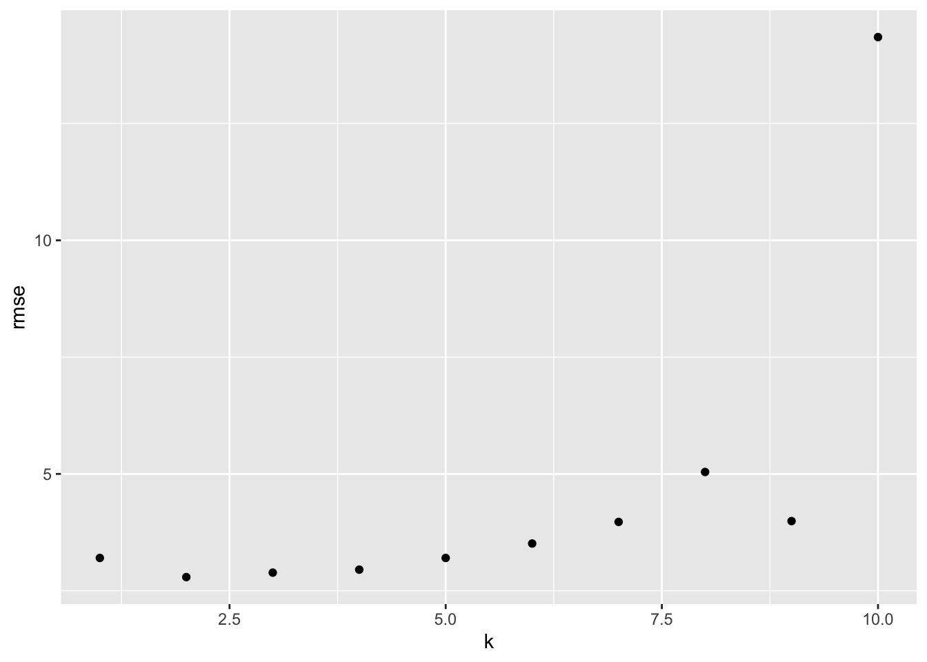
  • We use only the \(i\)th value in the predict() step.
• After computing \(n\) leave-one-out Yhat’s, we calculate the RMSE for the \(k\) and move to the next \(k\).

rmse <- rep(NA_real_,10)
Yhat <- rep(NA_real_, n)
for (k in 1:10) {
  for (i in 1:n) { # delete one at a time
    reg <- lm(mpg ~ poly(wt, k), data = mtcars[-i ,])
    Yhat[i] <- predict(reg, newdata = mtcars[i ,])
  }
  rmse[k] <- sqrt(mean((Yhat - mtcars$mpg) ^ 2))
}

We can plot the RMSE for each \(k\) as before.

ggplot(tibble(k = 1:10, rmse), aes(k, rmse)) +
  geom_point()

We see different pattern of RMSE. Note the scale of the \(y\) axis.

We can check the \(k\) with the minimum RMSE.

which.min(rmse)

[1] 2

min(rmse)

[1] 2.791732

• The recommended degree is now 2.
• The RMSE is higher but it is a more reliable estimate since we are using more of the data.

We can also look at the fitted values for the 10^th degree polynomial.

ggplot(bind_cols(mtcars, Yhat = Yhat), aes(wt, Yhat)) +
  geom_point(color = "red") +
  geom_smooth(se = FALSE) +
  geom_point(mapping = aes(wt, mpg), color = "purple") +
  ggtitle("LOOCV Predicted values (red) from the 10 degreee Polynomial")

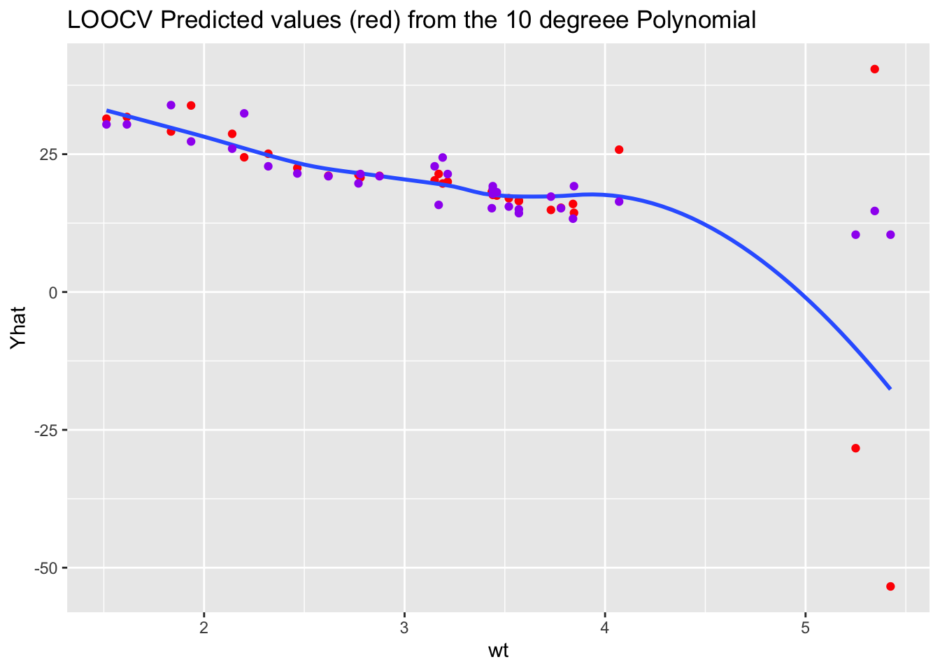
We no longer have the extreme values for the highest degree polynomial.

When we look at the chosen polynomial, we see

for (i in 1:n) { # delete one at a time
    reg <- lm(mpg ~ poly(wt, 2), data = mtcars[-i ,])
    Yhat[i] <- predict(reg, newdata = mtcars[i ,])
  }
ggplot(bind_cols(mtcars, Yhat = Yhat), aes(wt, Yhat)) +
  geom_point(color = "red") +
  geom_smooth(se = FALSE) +
  geom_point(mapping = aes(wt, mpg), color = "purple") +
  ggtitle("LOOCV Predicted values (red) from the 2 degreee Polynomial") ->
  plot_p
plot_p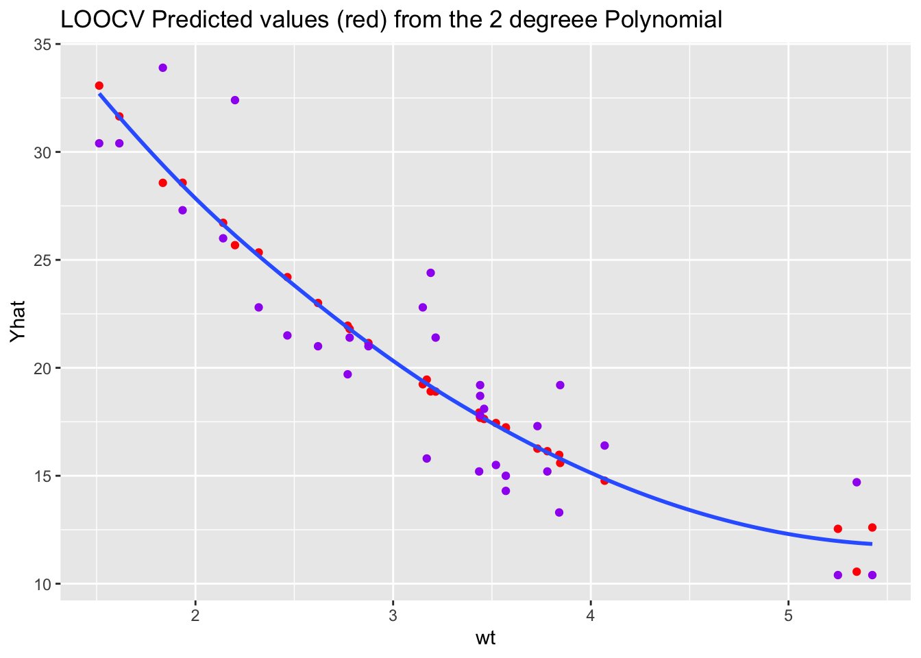

What do you notice about the \(\hat{y}\) for the recommended 2-degree polynomial?

• Are they all on the same curve like you are used to seeing with linear regression using the poly() function?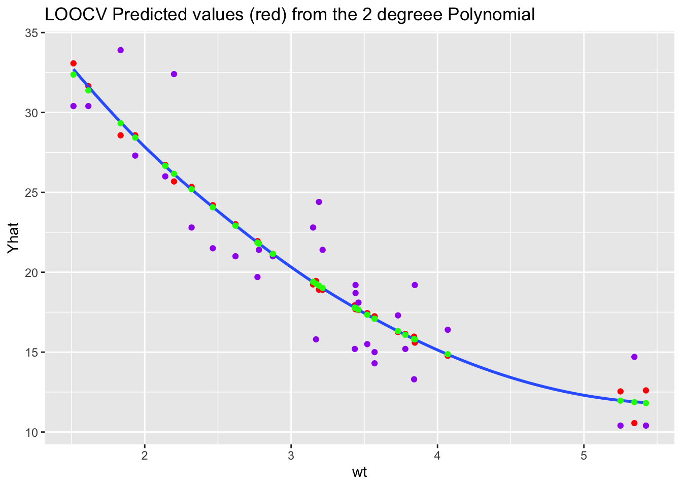

reg_p <- lm(mpg ~ poly(wt, 2), data = mtcars)
plot_p +
  geom_point(data = bind_cols(mtcars, p_fit = reg_p$fitted.values),
            mapping = aes(wt, p_fit), color = "green")

Why not?

We do not have to always write out these for loops for LOOCV. We will use the {boot} package later on which has functions we can use.

5.2.2 LOOCV for Classification

The above examples were regression problems using LOOCV for estimating the RMSE.

Earlier, the MASS::lda() function with CV = TRUE used this leave-one-out cross-validation method to produce the posterior probabilities for each category in a classification problem.

For classification, which does not have residuals that allow us to use RMSE, we can use LOOCV to estimate the prediction error rate using

\[ \frac{1}{n}\sum_{i=1}^n I_{\hat{y}_{i(-i)} \neq y_i} \]

where

\[ I_{\hat{y}_{i(-i)} \neq y_i} = \cases{ 1 \text{ if } \hat{y}_{i(-i)} \neq y_i \\ 0 \text{ otherwise }} \]

5.2.3 Implications of LOOCV for \(\text{Var}(\widehat{\text{RMSE}})\)

When you delete just one observation, are you really expecting the predictions to change much?

• Generally not.

A disadvantage of LOOCV is the results lead to strongly correlated components of \(\widehat{\text{MSE}}\) since every estimate uses almost the same data.

This affects the \(Var(\widehat{\text{MSE}})\).

Consider calculating a sample mean \(\bar{x}\) to estimate the population mean \(\mu\).

• Given \(x_1, x_2, \ldots, x_n\) with variance \(\sigma^2\), then

\[ \text{Var}(\bar{x}) = \text{Var} \left( \frac{1}{n}\sum_{i = 1}^n x_i\right) = \frac{1}{n^2}\sum_{i = 1}^n \text{Var}(x_i) =\frac{1}{n^2}(n \sigma^2) = \frac{\sigma^2}{n} \]

• See 24.3 - Mean and Variance of Linear Combinations for a proof of the algebra.

So, the larger the \(n\) the smaller the variance of the estimate which makes it a more reliable estimate.

But this is only true if the \(x_1, x_2, \ldots, x_n\) are uncorrelated, i.e., \(\text{Var}(\sum x_i) = \sum \text{Var}(x_i)\) only when all covariances \(\text{Cov}(x_i, x_j) = 0 \quad \forall i\neq j\).

However, if the components of RMSE are correlated, then the covariances among the residuals are each almost as large as the variance of the residuals.

The sum is now as follows:

\[ \text{Var}(\bar{x}) = \text{Var}\sum (\hat{y}_i - y_i)^2 = \sum \text{Var}(\,\,\underbrace{(\hat{y}_i - y_i)^2}_{e_i}\,\,) + \sum_i \sum_j \text{Cov}(e_i, e_j) \ \forall (i \neq j) \tag{5.1}\]

Equation 5.1 means the \(\text{Var}(\widehat{\text{MSE}})\) for LOOCV is much larger than desired.

What is the solution?

• Delete multiple observations at a time, not just one, to reduce the correlation!

5.3 \(K\)-Fold Cross-Validation

This is our third method of cross-validation after validation set and LOOCV.

\(K\)-fold Cross-Validation deletes a group of observations (called a fold) instead of just one observation.

• This will help de-correlate the components of \(\widehat{\text{MSE}}\)}.
• Which results in a more accurate estimator of MSE with lower variance that LOOCV.

Given a sample of size \(n\),

• we use a random selection to split the data into \(K\) groups (folds), then,
• we delete them one at a time to fit whatever model we are fitting, then,
• we use the data in the deleted fold to make predictions as seen in Figure 5.1, and
• we repeat the process \(K\) times to get \(K\) estimates for the predicted (test) error \(\text{MSE}_i = \hat{y}_{i(-K)}\)

Figure 5.1: First two steps in K-fold cross -validation.

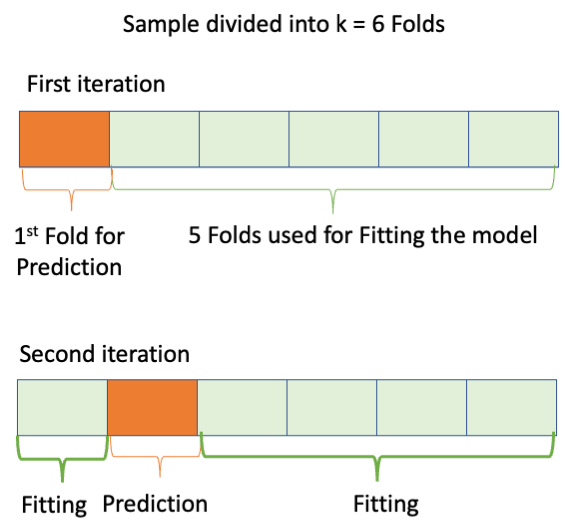
We then estimate the the cross validation MSE by averaging the “K” estimates of the test error as in Equation 5.2

\[ \widehat{\text{MSE}}_{CV} = \frac{1}{n}\sum(\hat{y}_{i (-K)} - y_i)^2 \tag{5.2}\]

Equation 5.2 is equivalent to equation 5.3 in the book as seen in Equation 5.3:

\[ \text{CV}_k = \frac{1}{k}\sum_{i=1}^k\text{MSE}_i \tag{5.3}\]

You can see K-fold is a generalization of LOOCV.

• When \(k=n\), then each fold is of size 1.
• If \(k = 2\), then each fold has size \(n/2\). Is this the same as using a validation set?
  • The first step is equivalent to a validation set approach.

What value of K?

Commonly used values of \(K\) are \(K=5\) and \(K=10\) based on empirical performance.

5.3.1 \(K\)-Fold Cross-Validation for Linear Regression

R has two packages commonly used for \(K\)-fold validation: {boot} and {bootstrap}.

• Let’s load them (Install them using the console if you need to) and also load {ISLR2} and the Auto data set.

library(tidyverse)
library(boot)
library(bootstrap)
library(ISLR2)
glimpse(Auto)

Rows: 392
Columns: 9
$ mpg          <dbl> 18, 15, 18, 16, 17, 15, 14, 14, 14, 15, 15, 14, 15, 14, 2…
$ cylinders    <int> 8, 8, 8, 8, 8, 8, 8, 8, 8, 8, 8, 8, 8, 8, 4, 6, 6, 6, 4, …
$ displacement <dbl> 307, 350, 318, 304, 302, 429, 454, 440, 455, 390, 383, 34…
$ horsepower   <int> 130, 165, 150, 150, 140, 198, 220, 215, 225, 190, 170, 16…
$ weight       <int> 3504, 3693, 3436, 3433, 3449, 4341, 4354, 4312, 4425, 385…
$ acceleration <dbl> 12.0, 11.5, 11.0, 12.0, 10.5, 10.0, 9.0, 8.5, 10.0, 8.5, …
$ year         <int> 70, 70, 70, 70, 70, 70, 70, 70, 70, 70, 70, 70, 70, 70, 7…
$ origin       <int> 1, 1, 1, 1, 1, 1, 1, 1, 1, 1, 1, 1, 1, 1, 3, 1, 1, 1, 3, …
$ name         <fct> chevrolet chevelle malibu, buick skylark 320, plymouth sa…

Calculate a linear regression of mpg on several variables using the glm function.

data(Auto)
reg <- glm(mpg ~ weight + year + displacement + cylinders + horsepower, data = Auto)

The glm() output object is suitable (has all the data needed) for using in a call to boot::cv.glm() which will compute the prediction error based on a \(K\)-fold cross validation of a generalized linear model.

5.3.1.1 Default \(K\)-Fold Cross-Validation

Run the cross validation with boot::cv.glm().

regCV <- cv.glm(Auto, reg)

Look at the help for cv.glm(). How is \(K\) chosen?

• The default is \(n\) so the default is equivalent to LOOCV.
• That means here it ran 392 linear regressions for us.

Glimpse the output.

glimpse(regCV)

List of 4
 $ call : language cv.glm(data = Auto, glmfit = reg)
 $ K    : num 392
 $ delta: num [1:2] 12 12
 $ seed : int [1:626] 10403 20 1654269195 -1877109783 -961256264 1403523942 124639233 261424787 1836448066 1034917620 ...

We see the original call and the \(K\) value (here the default).

delta is a vector of two estimates of cross-validation prediction error

1. The first is a raw estimate calculated as we saw previously: the average of the squared residuals.
2. The second is an adjusted cross-validation estimate based on \(K = n\).

• The adjustment is designed to compensate for the bias introduced by not using LOOCV.

regCV$delta

[1] 12.00069 12.00019

How can we use this?

Let’s see if we need all the variables in the model or we can do just as well without some.

5.3.1.2 Using a Reduced Model in Cross Validation

Let’s run a reduced model without displacment and cylinders.

reg2 <- glm(mpg ~ weight + year +  horsepower, data = Auto)
regCV2 <- cv.glm(Auto, reg2)
regCV2$delta

[1] 11.89897 11.89865

This is Prediction mean squared error. What does it mean that it is smaller?

• We did better without the additional variables.

• Confirm with anova() with test = "Chisq".

  • Our models are nested so ANOVA is fine.
  • We are using test = "Chisq" since we are using the general linear model and our results are based on deviance which is a Chi-Squared variable

aout <- anova(reg2, reg, test = "Chisq")
aout

Analysis of Deviance Table

Model 1: mpg ~ weight + year + horsepower
Model 2: mpg ~ weight + year + displacement + cylinders + horsepower
  Resid. Df Resid. Dev Df Deviance Pr(>Chi)
1       388     4565.7                     
2       386     4551.6  2   14.061   0.5509

• The high \(p\)-value (.55) suggests there is no evidence the larger (full) model is any better than the reduced without the two variables.

This was, by default, \(K=n\) or the same as LOOCV.

5.3.1.3 K=10-Fold Validation

Using the same glm() object for the reduced model, we just set K = 10 which is a common practice.

• Remember to set the seed for reproducibility. Why now compared to before?

set.seed(12)
regCV210 <- cv.glm(Auto, reg2, K = 10)
regCV210$delta

[1] 11.88056 11.86819

• Since 392/10 is not an integer, the second, adjusted value, of delta is adjusted to reduce the bias from uneven group sizes.

Just to check, set \(K=n\).

regCV2n <- cv.glm(Auto, reg2, K = 392)
regCV2n$delta

[1] 11.89897 11.89865

• Gives the same result as the default.

This was an example of \(K\)-fold cross validation in a regression context.

5.3.2 \(K\)-Fold Cross-Validation for Classification

In linear regression, R was calculating the sum of the squared residuals.

For classification, we don’t have results so we use the error classification rate.

Recall

\[ \widehat{\text{Error rate}} = \frac{1}{n}\sum I_{\hat{y}_{i(-i)} \neq y_i} \]

To do this, we will use a suitable Loss function.

• A loss function helps us evaluate performance by differentiating between the cost or loss for a wrong prediction and the benefit of a correct prediction.

Let’s define a Loss function \(L\) of the actual response value \(y\) and the estimated probability \(p\).

\[ \text{L}(y, p) = \cases{1 \qquad \text{if }\, y = 1 \text{ but }p \leq \text{threshold} \implies \hat{y} = 0 \\ \qquad \,\,\text{or }y = 0 \text{ but } p > \text{threshold}\implies \hat{y} = 1\\ \\ 0 \qquad \text{otherwise (we had correct prediction)}} \tag{5.4}\]

We can define Equation 5.4 as a function in R and use in glm() for logistic regression where we are predicting probabilities.

• Let’s use a threshold for \(p= 0.46\) from the Titanic example.
• We will calculate the mean of the Loss for a vector of values

L <- function(Y, p) {
  mean(1 * (Y == 1 & p <= .46) | (1 * (Y == 0 & p > .46)),
       na.rm = TRUE)
}

As an example, assume actual \(y_i= 1\) and an estimated \(p = .9\), the loss is

L(1, .9)

[1] 0

However, if actual \(y_i= 1\) and an estimated \(p = .3\), the loss is

L(1, .3)

[1] 1

Since we included mean() in our loss function, we can use a vector of predictions:

L(Y = c(1,1,1), p = c(.2, .6, .9))

[1] 0.3333333

Let’s load the Titanic data set from before.

titanic <- readr::read_csv("https://raw.githubusercontent.com/rressler/data_raw_courses/main/titanic_dalex.csv")
glimpse(titanic)

Rows: 2,207
Columns: 9
$ gender   <chr> "male", "male", "male", "female", "female", "male", "male", "…
$ age      <dbl> 42.0000000, 13.0000000, 16.0000000, 39.0000000, 16.0000000, 2…
$ class    <chr> "3rd", "3rd", "3rd", "3rd", "3rd", "3rd", "2nd", "2nd", "3rd"…
$ embarked <chr> "Southampton", "Southampton", "Southampton", "Southampton", "…
$ country  <chr> "United States", "United States", "United States", "England",…
$ fare     <dbl> 7.1100, 20.0500, 20.0500, 20.0500, 7.1300, 7.1300, 24.0000, 2…
$ sibsp    <dbl> 0, 0, 1, 1, 0, 0, 1, 1, 0, 0, 0, 0, 1, 0, 0, 0, 0, 0, 0, 0, 0…
$ parch    <dbl> 0, 2, 1, 1, 0, 0, 0, 0, 0, 0, 0, 0, 0, 1, 1, 0, 0, 0, 0, 0, 0…
$ survived <chr> "no", "no", "no", "yes", "yes", "yes", "no", "yes", "yes", "y…

Let’s check if embarked is a useful predictor variable.

• First convert survived to 0 or 1.

titanic$Y <- as.numeric(as.factor(titanic$survived)) - 1
table(titanic$survived)

  no  yes 
1496  711 

table(titanic$Y)

   0    1 
1496  711 

• Remove the NAs

titanic2 <- drop_na(titanic, Y, gender, age, class, fare, 
                    embarked)

• Fit a logistic regression model.

set.seed(1234)
titanic2 <- slice_sample(titanic2, n = 700) # reduce for speed in class
log_reg <- glm(Y ~ gender + age + class + fare + embarked, 
               data = titanic2, family = "binomial")

Now do the LOOCV and get the deltas.

cv.glm(titanic2, log_reg)$delta

[1] 0.1666763 0.1666713

• This is Mean Squared Error due to the default of treating as regression.

Now use the loss function.

cv.glm(titanic2, log_reg, cost = L)$delta

[1] 0.2400000 0.2399939

Since we used our Loss function, this is now the classification error rate.

We can set \(K\) as well.

• Set the seed for \(K=10\).

set.seed(123)
cv.glm(titanic2, log_reg, cost = L, K = 10)$delta

[1] 0.2400000 0.2415714

Let’s fit a model without embarked and compare.

log_reg <- glm(Y ~ gender + age + class + fare, 
               data = titanic2, family = "binomial")
set.seed(123)
cv.glm(titanic2, log_reg, cost = L, K = 10)$delta

[1] 0.2371429 0.2367143

Slightly lower error rate.

What if I delete class?

• Reset the seed for the CV to ensure you have the same data in each fold.

log_reg <- glm(Y ~ gender + age  + fare, 
               data = titanic2, family = "binomial")
set.seed(123)
cv.glm(titanic2, log_reg, cost = L, K = 10)$delta

[1] 0.2585714 0.2598571

Adjusted error rate went up so there is some value in class.

Important

You can use cross validation to compare models for any kind of tuning.

5.4 Jackknife: Another Use of LOOCV

Jackknife is a method for reducing bias. It was developed in 1949 as mentioned earlier.

Since MSE is the sum of Bias and Variance, we would like to reduce the Bias without increasing the Variance.

If \(E[\hat{\theta}] = \theta\) then we say \(\hat{\theta}\) is unbiased estimator of \(\theta\).

• Note that \(E[\hat{\theta}]\) is the average over all possible samples of the population - which is hard to do.

Under the standard linear regression assumptions, our estimators for the \(\beta\)s are unbiased.

However, suppose \(\theta\) is the population maximum. If we have a \(\hat{\theta}\) from a sample, is it unbiased?

• Usually not. It will usually underestimate the population maximum since many samples do not include the true population maximum.

5.4.1 Biased Estimators

Assume we have some population statistic, \(\theta\), which is unknown, and we want to estimate it with an estimator \(\hat{\theta}\).

• \(\theta\) could be the mean, the variance, the slopes, MSE, TPR, maximum, minimum, etc..
• We calculate \(\hat{\theta}\) from the sample data.

Let’s define the bias of \(\hat{\theta}\) as:

\[ \text{Bias}(\hat{\theta}) = E[\hat{\theta}] - \theta \tag{5.5}\]

We can collect multiple samples from a population and each sample will get its own \(\hat{\theta}_i\).

The expected value of \(\hat{\theta}\) (denoted by \(E[\hat{\theta}]\)) is the average of all possible \(\hat{\theta}_i\) from all possible samples of our population.

We would love for \(E[\hat{\theta}]\) to be \(\theta\).

• If \(E[\hat{\theta}]=\theta \iff \text{Bias}(\hat{\theta}) = 0\), we call \(\hat{\theta}\) an unbiased estimator of \(\theta\).

However, for many \(\theta\), there is no unbiased estimator for a given population.

5.4.1.1 Example: \(\text{logit}(p)\) has no unbiased estimator

The sample proportion \(\hat{p}\) is a unbiased estimator for the parameter \(p\) of a Binomial distribution

However, the logit of the proportion, \(\text{logit}(\hat{p}) = \ln(\hat{p}/(1-\hat{p}))\), is a nonlinear function of the proportion \(\hat{p}\) and we can show it must be biased.

• Given a sample of independent \(X_1, X_2, \ldots X_n\) from a Binomial distribution with parameter \(p\), the distribution function of the \(X\) is the product of the probabilities which can be simplified to a functio of \(p\).

\[ p(X_1, X_2, \ldots X_n) = \prod p(X_i) = p^{\sum X_i}(1-p)^{(n-\sum X_i)} \rightarrow \text{a polynomial of }p \]

• Let \(\hat{\theta}\) represent any function of the sample \(X_1, X_2, \ldots X_n\).
• We can calculate the expected value of \(\hat{\theta}\) as the sum (integral) of the possible values of \(\hat{\theta}\) times the probability of each value.

\[ E[\hat{\theta}] = \sum\underbrace{\hat{\theta}(X_1, X_2, \ldots X_n)}_{\text{Does not depend on }p}\,* \underbrace{p(X_1, X_2, \ldots X_n)}_{\text{a polynomial of }p} \tag{5.6}\]

• The first term of Equation 5.6 is a function of the sample values and does not depend upon \(p\).
• The second term of Equation 5.6 is a polynomial of \(p\).

Therefore, Equation 5.6 shows the expected value of an estimator, \(\hat{\theta}\), of any statistic of a population with a binomial distribution, can only be a polynomial.

Since the logit function \(\text{logit}(p) = \ln(p/(1-p))\) is Not a polynomial, it follows that

• \(E[\text{logit}(p)] \neq \text{logit(p)}\) so
• the parameter \(\theta = \text{logit}(p)\) can’t have an unbiased estimator.

Note

Since our goal is reducing Bias + Variance, sometimes, even when there is an unbiased estimator, we might prefer using a biased estimator with other nice properties such as reducing the MSE.

• Foreshadowing Ridge Regression and Lasso - shrinkage methods of estimation which intentionally sacrifice unbiasedness to reduce variance.

When we are using a biased estimator, we can use Jackknife as a method to reduce the bias.

5.4.2 Goals for Handling Bias

1. Given an estimator \(\hat{\theta}\), estimate the \(\text{Bias}(\hat{\theta})\) (the true value of the parameter is unknown and the expected value of the estimator \(\hat{\theta}\) is unknown since we have only one sample).
2. Check if the estimator is unbiased by seeing if \(\text{Bias}(\hat{\theta}) = 0\).
3. If not, and \(\hat{\theta}\) is biased, try to reduce its bias, or,
4. If possible, derive a new unbiased estimator.

Note

In 1989, Doss and Sethuraman proved the following caution about bias reduction:

If there is no unbiased estimator \(\hat{\theta}\), but you can construct a sequence of estimators such that \(\text{Bias}(\hat{\theta}) \rightarrow 0\), i.e., using repeated jackknifes, \(\text{Variance}(\hat{\theta}) \rightarrow \infty\).

5.4.3 Derivation of Jackknife

Quenouille noticed the bias of an estimator tends to reduce as the sample size \(n\) increases.

That suggested using a power series to represent the unknown function for the bias of \(\hat{\theta}\):

\[ \text{Bias}(\hat{\theta}) = \overbrace{\frac{a_1}{n} + \frac{a_2}{n^2} + \frac{a_3}{n^3} + \cdots}^{\text{the Bias}} \qquad \implies \text{of order} \frac{1}{n} \tag{5.7}\]

where \(a_1, a_2, a_3, \ldots\) are some coefficients that are unknown.

Note

We use Big \(O\) notation to represent what happens to the results as \(n \rightarrow \infty\).

Here it means that as \(n \rightarrow \infty\), the \(a_1/n\) term will be the largest term, regardless of the value of any \(a_i\), as the other terms will approach 0 much faster.

• If \(a_i = 0 \, \forall i\) then we can say \(\hat{\theta}\) is unbiased.

We can then use Equation 5.5 to express the expected value of \(\hat{\theta}\) as \(\theta\) + the bias, or,

\[ E[\hat{\theta}]=\theta + \overbrace{\frac{a_1}{n} + \frac{a_2}{n^2} + \frac{a_3}{n^3} + \cdots }^{\text{the Bias}} \tag{5.8}\]

Now let’s apply jackknife, a LOOCV approach.

• Delete one \(X_i\) at a time, so the sample is of size \(n-1\) and calculate \(\hat{\theta}_{(-i)}\).
• Do it for each \(X_i\) and calculate the average, denoted as \(\hat{\theta}_{(.)}\).

\[ \text{Average: }\equiv \,\hat{\theta}_{(.)}= \frac{1}{n} \sum_{i=1}^n \hat{\theta}_{(-i)} \]

That gives us an expected value of:

\[ E[\hat{\theta}_{(.)}]=\theta + \overbrace{\frac{a_1}{n-1} + \frac{a_2}{(n-1)^2} + \frac{a_3}{(n-1)^3} + \cdots }^{\text{the Bias}} \tag{5.9}\]

Let’s look at Equation 5.8 and Equation 5.9 together and see if we can reduce the variance by combining them in a way that eliminates the first term of the bias, the \(O(n)\) term.

Start with the following

\[ \begin{align} E[\hat{\theta}] & = \theta + \quad\frac{a_1}{n} \,\,\,+ \quad\,\frac{a_2}{n^2} \quad\,\,\, +\quad \, \frac{a_3}{n^3} \quad \,+ \cdots \\ \\ E[\hat{\theta}_{(.)})]&= \theta + \,\frac{a_1}{n-1} + \frac{a_2}{(n-1)^2} + \frac{a_3}{(n-1)^3} + \cdots \end{align} \]

Multiply the first equation by \(n\) on both sides and the second equation by \((n-1)\) on both sides.

\[ \begin{align} n*E[\hat{\theta}] & = \,\,\,\,\,\,n\theta \quad \,\,+ \frac{a_1}{1} \,\,\,+ \quad\,\frac{a_2}{n} \quad\, +\quad \, \frac{a_3}{n^2} \quad \,+ \cdots \\ \\ (n-1)*E[\hat{\theta}_{(.)})]&= (n-1)\theta + \,\frac{a_1}{1} + \frac{a_2}{(n-1)^1} + \frac{a_3}{(n-1)^2} + \cdots \end{align} \tag{5.10}\]

Now subtract the bottom of Equation 5.10 from the top:

1. Subtracting the left side Equation 5.10 yields a linear combination of expectations which we can combine into one expectation:

\[ nE[\hat{\theta}] - (n-1)E[\hat{\theta}_{(.)}] = E[n\,\hat{\theta} - (n-1)\hat{\theta}_{(.)}] \]

2. Combining the left with the right gives us:

\[ \begin{align} E[n\,\hat{\theta} - (n-1)\hat{\theta}_{(.)}] & = \bigg(n\theta - (n-1)\theta\bigg) + (a_1 - a_1) + \left(\frac{a_2}{n} - \frac{a_2}{(n-1)}\right) + \cdots\\ \\ & = \theta + 0 +\frac{(n-1)a_2 - na_2}{n(n-1)} + \cdots\\ \\ &= \theta + \quad \frac{-a_2}{n^2-n} \,\,\,+ \cdots \\ \\ E[\hat{\theta}_{JK}] =E[ n\hat{\theta} - (n-1)\hat{\theta}_{(.)}]&= \theta + \qquad\, \frac{b_2}{n^2}\quad\,+\cdots \qquad \implies \text{of order } \frac{1}{n^2} << \frac{1}{n} \end{align} \tag{5.11}\]

So the bias has been reduced as the \((1/n^2)\) will be smaller in magnitude than the \(1/n\) terms from Equation 5.7.

The left side of Equation 5.11 is called the Jackknife Estimator, \(\hat{\theta}_{JK}\) and we will use the following formula for it to reduce the bias of an original estimate.

\[ \hat{\theta}_{JK}= n\hat{\theta} - (n-1)\hat{\theta}_{(.)} \tag{5.12}\]

Note

As seen in Equation 5.11, \(\hat{\theta}_{JK}\) has a smaller bias than the original \(\hat{\theta}\).

Bias may be positive or negative.

As a result, \(\hat{\theta}_{JK}\) may be smaller or larger than the original \(\hat{\theta}\) to correct the over-estimation or under-estimation of the original estimator.

Example: If we have a sample size of \(1000\), then \(\hat{\theta}\) has a bias of order \(b/1000\) and \(\hat{\theta}_{JK} = n\hat{\theta} - (n-1)\hat{\theta}_{(.)}\) has a bias of order \(b/(1000)^2\).

5.4.4 Summary of the Steps in Jackknife

The method has three steps once you have calculated the original (potentially-biased) estimator \(\hat{\theta}\) using all \(n\) values in the sample.

1. Calculate the \(n\) leave-one-out estimates \(\hat{\theta}_{(-i)}\)
2. Average these leave-one-out estimates to get \(\hat{\theta}_{(.)}\)
3. Use the jackknife formula from Equation 5.12 \(\hat{\theta}_{JK} = n\,\hat{\theta} - (n-1) \hat{\theta}_{(.)}\) to calculate the less-biased result.

5.4.5 Example: Using Jackknife to Estimate the Population Maximum

We want to estimate the height of the tallest person on earth (in inches)

• We take a sample of 4 people and get 65, 70, 72, and 65.
• The max of our sample is 72 inches. Is this a good estimate?
• It appears biased as \(E[\hat{\theta}] < \theta\) so it underestimates the population maximum

Let’s apply Jackknife

1. Delete one at a time

• Delete 65, gives a sample of 70, 72, 65 so \(\hat{\theta}_{-1} = 72\)
• Delete 70, gives a sample of 65, 72, 65 so \(\hat{\theta}_{-2} = 72\)
• Delete 72, gives a sample of 65, 70, 65 so \(\hat{\theta}_{-3} = 70\)
• Delete 65, gives a sample of 65, 70, 72 so \(\hat{\theta}_{-4} = 72\)

2. Now calculate the average: \(\hat{\theta}_{.} = \frac{72 + 72 + 70 + 72}{4} = 71.5\)

3. Calculate the jackknife estimate. \(n = 4\) so

\[ \begin{align} \hat{\theta}_{JK} &= n\,\hat{\theta} - (n-1) \hat{\theta}_{(.)} \\ &= 4 * 72 - 3 * 71.5 \\ &= 288 - 214.5 \\ &= 73.5 \end{align} \]

Note. It is still biased but it has less bias than before.

Let’s estimate the amount of bias of the original \(\hat{\theta}\).

\[ \begin{align} \widehat{\text{Bias}}(\hat{\theta})&= \hat{\theta} - \hat{\theta}_{JK} \\ &= 72 - 73.5 \\ &= -1.5 \end{align} \]

5.4.6 Example: Using bootstrap::jackknife() to Estimate the Maximum of mtcars$mpg.

We will use the jackknife() function from the {bootstrap} package for Jackknife methods.

library(bootstrap)

bootstrap::jackknife() requires us to define a function to calculate our estimator \(\theta\) since we can use the jackknife for any kind of estimator we want.

Let’s create a function to find the maximum of a sample.

my_max <- function(x) max(x, na.rm = TRUE)

Let’s look at mpg in the mtcars data set.

data("mtcars")
summary(mtcars$mpg)

   Min. 1st Qu.  Median    Mean 3rd Qu.    Max. 
  10.40   15.43   19.20   20.09   22.80   33.90 

nrow(mtcars)

[1] 32

Use the bootstrap::jackknife() function with the data and the my_max function for \(\theta\).

• Note we are using the name of the function my_max and not calling it using the my_max().

jk <- jackknife(x = mtcars$mpg, theta = my_max)
jk

$jack.se
[1] 1.453125

$jack.bias
[1] -1.453125

$jack.values
 [1] 33.9 33.9 33.9 33.9 33.9 33.9 33.9 33.9 33.9 33.9 33.9 33.9 33.9 33.9 33.9
[16] 33.9 33.9 33.9 33.9 32.4 33.9 33.9 33.9 33.9 33.9 33.9 33.9 33.9 33.9 33.9
[31] 33.9 33.9

$call
jackknife(x = mtcars$mpg, theta = my_max)

The jack.values are the 32 estimates \(\hat{\theta}_{(-i)}\) with one value deleted.

Compare them to the original values.

table(jk$jack.values)

32.4 33.9 
   1   31 

table(mtcars$mpg)

10.4 13.3 14.3 14.7   15 15.2 15.5 15.8 16.4 17.3 17.8 18.1 18.7 19.2 19.7   21 
   2    1    1    1    1    2    1    1    1    1    1    1    1    2    1    2 
21.4 21.5 22.8 24.4   26 27.3 30.4 32.4 33.9 
   2    1    2    1    1    1    2    1    1 

Let’s get the mean \(\hat{\theta}_{(.)}\) and then calculate the jackknife estimate using Equation 5.12.

n <- nrow(mtcars)
jk_dot <- mean(jk$jack.values)
theta_jk <- n * max(mtcars$mpg) - (n - 1) * jk_dot
theta_jk 

[1] 35.35313

Now we can get the bias.

max(mtcars$mpg) - theta_jk

[1] -1.453125

Or we can calculate the original \(\hat{\theta}\) and subtract the bias to get the jackknife estimate.

max(mtcars$mpg) - jk$jack.bias

[1] 35.35312

5.4.6.1 Exercise: Calculate the Jackknife estimate for the Minimum of mtcars$mpg.

• What do you notice about this estimate?

my_min <- function(x) min(x, na.rm = TRUE)
jkm <- jackknife(x = mtcars$mpg, theta = my_min)
jkm

n <- nrow(mtcars)
jkm_dot <- mean(jkm$jack.values)
theta_jkm <- n * min(mtcars$mpg) - (n - 1) * jkm_dot
theta_jkm
min(mtcars$mpg) - theta_jkm

sort(mtcars$mpg)

5.4.7 Example: Estimate the Population Variance

We can calculate the variance of a sample using the R var() function.

var(mtcars$mpg)

[1] 36.3241

Let’s define a function to calculate a sample variance based on the definition of a population variance:

my_var <- function(x) mean((x - mean(x, na.rm = TRUE))^2)
my_var(mtcars$mpg)

[1] 35.18897

Why do we get a different result?

The standard estimator of variance is

\[ \hat{\sigma}^2 = s^2 = \frac{1}{n-1}\sum_i^n(x_i - \bar{x})^2 \]

This is what R uses in var() as it divides by \((n-1)\) to make the output unbiased.

• Dividing by \((n-1)\) makes this an example of an unbiased estimator since \(E[s^2] = \sigma^2\)

In my formula we used the mean() which means we used \(1/n\) so my_var() was biased as it underestimated the variance.

Let’s calculate the jackknife output for my_var().

jk <- jackknife(mtcars$mpg, my_var)
jk

$jack.se
[1] 8.75157

$jack.bias
[1] -1.135128

$jack.values
 [1] 36.29657 36.29657 36.07967 36.26701 36.25971 36.19215 35.20755 35.70572
 [9] 36.07967 36.29769 36.14939 35.87055 36.06479 35.52766 33.19709 33.19709
[17] 35.35648 31.27867 32.78502 29.97409 36.25796 35.62237 35.52766 34.78862
[25] 36.29769 34.59340 35.16129 32.78502 35.71109 36.31902 35.46119 36.26701

$call
jackknife(x = mtcars$mpg, theta = my_var)

Let’s take the original estimate and subtract the bias calculated by jackknife():

my_var(mtcars$mpg) - jk$jack.bias

[1] 36.3241

We get the same value as the unbiased estimator.

The jackknife method allows us to create an unbiased estimate.

5.4.8 Example: Using Jackknife with Vaccine Trial Data

We want to use data from a vaccine trial to estimate its effectiveness in terms of the probability of creating antibodies after the vaccine.

Say we have a sample of 20 and the first \(X_1, X_2, \ldots, X_{13} = 1\) and \(X_{14}, X_{15}, \ldots, X_{20} = 0\)

We use the sample proportion to estimate \(p\) so we estimate \(\hat{p} = 13/20\). This is a unbiased as it is also a sample mean (linear combination of the samples).

We want to estimate the logit of \(p\), \(\ln(\frac{p}{1-p})\), which is a non-linear function of \(p\).

That means \(\widehat{\text{Logit}}(p) = \ln\left(\frac{\hat{p}}{(1-\hat{p})}\right)\) may be biased.

5.4.8.1 Jesen’s Inequality

You may have heard of Jensen’s inequality which states several properties about the expectation of a function \(g(x)\).

\[ \begin{align} 1. \qquad E[g(x)] &\geq g(E[x]) \iff \quad g(x) \text{ is convex} \iff \text{second derivative is postive: smile} \implies \text{Overestimates}\\ \\ 2. \qquad E[g(x)] &\leq g(E[x]) \iff \quad \text{ is concave} \iff \text{second derivative is negative: frown}\implies \text{Underestimates}\\ \\ 3. \qquad E[g(x)] &= g(E[x]) \iff \quad \text{ is linear} \iff \text{second derivative} = 0\implies \text{Unbiased} \end{align} \tag{5.13}\]

Equation 5.13 shows why the sample mean is unbiased, as it is a linear function of the sample values.

For our sample standard deviation, the \(\sqrt{}\) function is concave. Thus case 2 from Equation 5.13 applies and we have:

\[ E[s] = E[\sqrt{s^2}]\quad \leq \quad \sqrt{E[s^2]} = \sqrt{\sigma^2} = \sigma \]

This means the standard deviation underestimates the population standard deviation \(\sigma\).

We saw that we could use jackknife to correct for this bias.

What about the logit function? Is it Convex or Concave?

• Let’s take the first and second derivative of the function

\[ \begin{align} \text{Logit}(p) &= \ln\bigg(\frac{p}{(1-p)}\bigg) = \ln(p) - \ln(1-p)) \\ \\ \text{first derivative } \text{Logit}'(p)&=\,\,\,\,\, \frac{1}{p} - \frac{-1}{1-p} = \frac{1}{p} + \frac{1}{1-p}\\ \\ \text{second derivative }\text{Logit}''(p) &= \frac{-1}{p^2} + \frac{1}{(1-p)^2} \end{align} \]

This will be positive or negative depending upon the value of \(p > .5\).

suppressMessages(library(tidyverse))

df <- tibble(p = rep(1:1000)/1000, 
             y = log(p/(1 - p))
             )

 ggplot(df, aes(p, y)) +
   geom_line() +
   annotate("text", x = .7, y = 3, label = "Convex\n so Overestimates", size = 5) +
   annotate("text", x = .25, y = -3, label = "Concave\n so Underestimates", size = 5) +
   geom_vline(xintercept = .5, color = "red", lty = 2) +
   ylab(latex2exp::TeX("Logit$(p) = \\frac{p}{(1-p)}$"))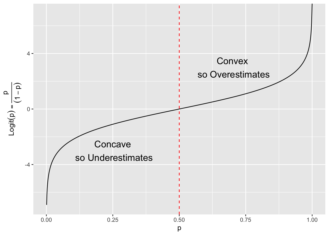

Figure 5.2: A logit curve is concave for p < 0.5 and convex for p > 0.5.

5.4.8.2 Back to the Example

Let’s go through the Jackknife steps:

Step 1: Delete 1 at a time and calculate the estimate \(\hat{\theta}_{(-1)}, \ldots, \hat{\theta}_{(-n)}\)

Step 2: Average the results: \(\hat{\theta}_{(.)} = \frac{1}{n} \sum \hat{\theta}_{(-i)}\)

Step 3: Apply the jackknife formula \(\hat{\theta}_{JK} = n\hat{\theta} - (n-1) \hat{\theta}_{(.)}\)

Step 1: We delete one at a time and we get 20 estimates of the sample logit. With our sample of 13 1’s and 7 0’s we can simplify:

• 13 times we delete a 1 to get \(\hat{p}_i = 12/19 i \in {1, 13}\) so \(\text{Logit}(\hat{p}_{1's}) = \ln\bigg(\frac{12/19}{7/19}\bigg)\)
• 7 times we delete a 0 to get \(\hat{p}_i = 13/19\) so \(\text{Logit}(\hat{p}_{0's}) = \ln\big(\frac{13/19}{6/19}\bigg)\)

Step 2: Average

\[ \hat{\theta}_{(.)} = \frac{13 * \ln(12/7) + 7 * \ln(13/6)}{20} = 0.621 \]

Step 3. The original \(\hat{p}\) was 0.65 with \(\text{Logit}(\hat{p}) =\) 0.6190392, so we use Equation 5.12 to get

\[ \hat{\theta}_{JK} =20 * \ln(.65/.35) - 19*.621 = 0.582 \]

To estimate the bias of \(\hat{\theta}\), use \(\hat{\theta} - \hat{\theta}_{JK} = 0.619 - .582= .037\)

Conclusion: for this \(p\) the sample logit overestimates the true logit and our new estimate should be less biased.

• Refer back to Figure 5.2.
• Since \(\hat{p} > 0.5\), \(\hat{\theta}\) is on the convex (right) side of the curve, which means \(\hat{\theta}\) overestimates the \(\theta\).

5.5 Bootstrap

Bootstrap is another method of evaluating the performance of a model/method and generating confidence intervals.

• One applies the same algorithm or method to the sample as the one applied to the population to calculate the parameter of interest.
• This allows us to estimate the properties of the parameter.
• We build an algorithm to calculate the property for the population and then apply it to the sample.
• The Bootstrap is especially useful in smaller sample sizes.

Let’s say we want to know the \(\text{Var}(\hat{\theta})\) for some \(\theta\) for the population.

• We would have to draw all possible samples to truly know the value of \(\text{Var}(\hat{\theta})\).
  • We calculate \(\hat{\theta}\) for each sample and then calculate the \(\text{Var}(\hat{\theta})\).
  • Undoable for samples of any size.

Bootstrap replaces the population with our sample and then generates (all possible) a large number of samples of size \(n\) by sampling with replacement.

• Sampling with replacement means the samples are independent.
• \(n^n\) possible bootstrap samples. - Again too large to get all possible samples.
• We just get a large \(n\) number of samples, often \(n = 10,000 \text{ up to } 100,000\).

We compute our statistics from each sample.

We then use the \(n\) estimates to get a bootstrap distribution of \(\hat{\theta}\).

• This allows us to calculate any property (statistic) of the distribution of the parameter of interest.
• The statistic may be the mean, the variance, quantiles, etc..

One can use the distribution of \(\hat{\theta}\) to create a bootstrap confidence interval for the true value of \(\theta\).

5.5.1 Example: Calculating a Bootstrap Distribution “By Hand” Using R

We want to calculate the properties of the sample median for mtcars$mpg.

We’ll use 10,000 samples.

median(mtcars$mpg)

[1] 19.2

n_samp <- 10000
bootstrap_medians <- rep(NA_real_, n_samp)

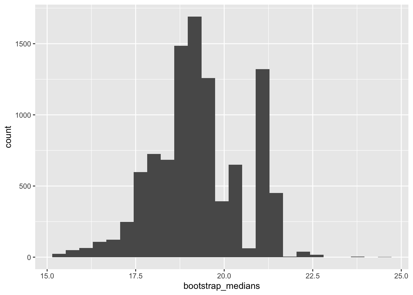
Let’s generate the samples and calculate the median for each sample

set.seed(1234)
n <- length(mtcars$mpg)
for (i in seq_along(bootstrap_medians)) {
  x <- sample(mtcars$mpg, n, replace = TRUE)
  bootstrap_medians[i] <- median(x, na.rm = TRUE)
}
head(bootstrap_medians, n = 10)

 [1] 19.20 18.95 19.20 19.70 21.00 18.65 20.35 17.80 20.10 18.95

We can now plot the distribution of our bootstrap estimates of the median.

ggplot(tibble(bootstrap_medians), aes(bootstrap_medians)) +
  geom_histogram(bins = 25)

We can calculate various statistics as well.

mean(bootstrap_medians)

[1] 19.28492

median(bootstrap_medians)

[1] 19.2

sd(bootstrap_medians)

[1] 1.262394

var(bootstrap_medians)

[1] 1.593638

quantile(bootstrap_medians, probs = .975)

97.5% 
 21.4 

To calculate confidence intervals:

quantile(bootstrap_medians, probs = c(.025, .975)) # 95%

 2.5% 97.5% 
 16.8  21.4 

quantile(bootstrap_medians, probs = c(.005, .995)) # 99%

 0.5% 99.5% 
 15.8  22.1 

ggplot(tibble(bootstrap_medians), aes(bootstrap_medians)) +
  geom_histogram(bins = 50) +
  geom_vline(xintercept = quantile(bootstrap_medians, probs = c(.025)),
             color = "red", lty = 2) +
  geom_vline(xintercept = quantile(bootstrap_medians, probs = c(.975)),
             color = "red", lty = 2) +
    geom_vline(xintercept = quantile(bootstrap_medians, probs = c(.005)),
             color = "green", lty = 2) +
  geom_vline(xintercept = quantile(bootstrap_medians, probs = c(.995)),
             color = "green", lty = 2)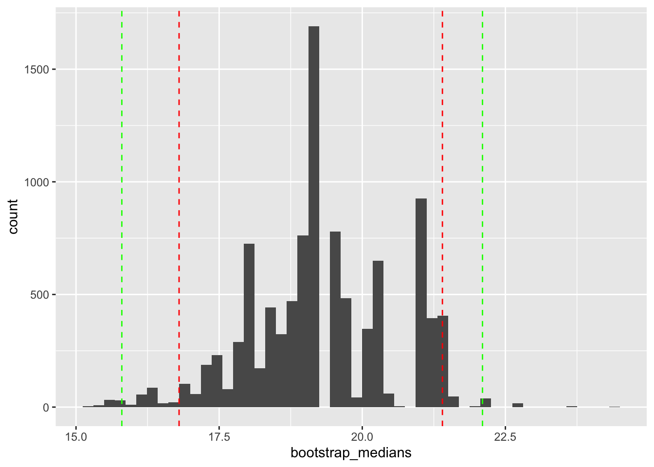

This has the same interpretation as usual.

• If we repeat the procedure many times, we expect the true population median to be in 95% (or 99%) of the samples.
• We just don’t know if it is in this sample.

This ability to generate a distribution and confidence intervals for any statistic makes the bootstrap a popular procedure.

5.5.2 Example of Calculating the Sample Median Using the {boot} Package

This is the same package we used for cross-validation.

• We used {bootstrap} for jackknife.

library(boot)

We again have to define a function for our estimator and that function must have two arguments:

• The data, and,
• A vector of indices for a subset (or sub-sample) of the data.

Let’s define a function for the median of a sample.

my_median <- function(x, subsample) median(x[subsample], na.rm = TRUE)

We can compare our function to the R median function using the entire sample.

median(mtcars$mpg)

[1] 19.2

my_median(mtcars$mpg, 1:length(mtcars$mpg))

[1] 19.2

This only gives us one sample estimate of the sample median. We can’t calculate any statistics about our estimator with one sample.

Now set up to run with bootstrap samples

• Set the seed.

set.seed(1234)
n <- length(mtcars$mpg)
my_median(mtcars$mpg, sample(n, n, replace = TRUE))

[1] 19.2

Let’s use boot::boot() to generate our 10,000 bootstrap samples

set.seed(1234)
b_out <- boot::boot(mtcars$mpg, my_median, R = 10000)
b_out

ORDINARY NONPARAMETRIC BOOTSTRAP


Call:
boot::boot(data = mtcars$mpg, statistic = my_median, R = 10000)


Bootstrap Statistics :
    original  bias    std. error
t1*     19.2  0.0881    1.272659

broom::tidy(b_out)

# A tibble: 1 × 3
  statistic   bias std.error
      <dbl>  <dbl>     <dbl>
1      19.2 0.0881      1.27

The more samples, the more the estimate converges to the maximum likelihood estimate.

This is a non-parametric method. We have not made any assumptions about the distribution of \(\hat{\theta}\).

The content of b_out has several elements in the list

class(b_out)

[1] "boot"

b_out$t0        # the original estimate

[1] 19.2

b_out$t[1:10]         # the vector of individual bootstrap estimates

 [1] 21.40 19.85 20.35 20.10 20.35 16.10 21.00 18.40 17.95 18.40

b_out$statistic # the structure of the function (formals, body, and environment)

function(x, subsample) median(x[subsample], na.rm = TRUE)
<bytecode: 0x10af431f8>

ggplot(tibble(b_out$t), aes(b_out$t)) +
  geom_histogram(bins = 25)

What if we want the inter-quartile range?

• This is a robust estimator of the spread - not heavily influenced by outliers.

ggplot(tibble(b_out$t), aes(1, b_out$t)) +
  geom_boxplot()

quantile(b_out$t, probs = .75) - quantile(b_out$t, probs = .25)

 75% 
1.95 

5.5.3 Example: Pfizer BioNTech COVID-19 Vaccine

The clinical trial include 44,000 participants, randomized into two equal groups.

• Double blind study.
• 22,000 vaccine and 22,000 got the placebo and neither patients or doctors know who is in which group.

Result - 170 participants contacted Covid-19.

• 162 from the placebo group
• 8 from the vaccine group.

One can claim from these results that the vaccine reduces the chance of infection by a factor of \(20=\frac{162}{8}\).

Let’s use this ratio as our estimate of interest, \(\hat{\theta}\).

\[ \hat{\theta} = \frac{\text{count placebo patients infected}}{\text{count vaccine patients infected}} \]

Critics claimed that with only 170 cases the results were not valid.

Let’s calculate a 95% confidence interval to give a measure of the uncertainty associated with the “single number” \(\hat{\theta}\).

Create a data frame of the trial data of patients and cases.

• patients = 1 means vaccine, and,
• cases = 1 means infected

trial <- data.frame(
patients =  c(rep(1, 22000), rep(0, 22000)), # patients (vaccine, placebo)
cases =  c(rep(1, 8), rep(0, 21992), rep(1, 162), rep(0, 21838))
) 
head(trial)

  patients cases
1        1     1
2        1     1
3        1     1
4        1     1
5        1     1
6        1     1

Define the function for our estimate \(\hat{\theta}.\)

ratio <-  function(data, sample) {
  p1 <- sum(data[sample,]$cases == 1 & data[sample,]$patients == 0) / 
    sum(data[sample,]$patients == 0)
  p2 <- sum(data[sample,]$cases == 1 & data[sample,]$patients == 1) /
    sum(data[sample,]$patients == 1)
  p1/p2 #infected placebo /infected vaccine
}

Let’s get the overall sample estimate and try a sub sample.

set.seed(123)
ratio(trial)

[1] 20.25

ratio(trial, sample(1:40000, 3000))

[1] 6.021308

We can see a range of results.

Let’s compare across different number of samples.

• This can take a long time with 10,000 samples.

set.seed(123)
boot::boot(trial, ratio, 100)

ORDINARY NONPARAMETRIC BOOTSTRAP


Call:
boot::boot(data = trial, statistic = ratio, R = 100)


Bootstrap Statistics :
    original   bias    std. error
t1*    20.25 3.865687     11.1073

boot::boot(trial, ratio, 1000)

ORDINARY NONPARAMETRIC BOOTSTRAP


Call:
boot::boot(data = trial, statistic = ratio, R = 1000)


Bootstrap Statistics :
    original  bias    std. error
t1*    20.25     Inf         NaN

b_out <- boot::boot(trial, ratio, 10000)
b_out

ORDINARY NONPARAMETRIC BOOTSTRAP


Call:
boot::boot(data = trial, statistic = ratio, R = 10000)


Bootstrap Statistics :
    original  bias    std. error
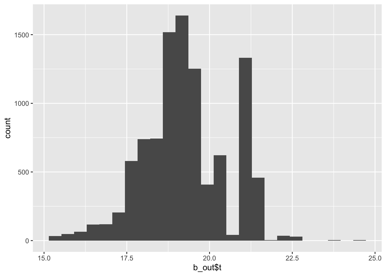
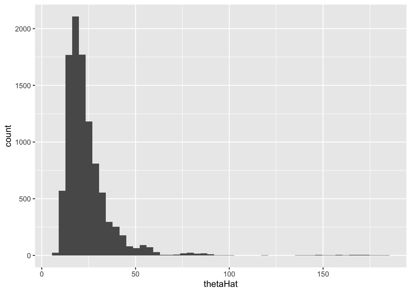
t1*    20.25     Inf         NaN

• Note the NAN’s or inf in the results for bias and standard error means some samples had 0 in the denominator since the sample didn’t select any of the positive cases.

Let’s plot the histogram of our 10,000 samples:

suppressMessages(library(ggplot2))
ggplot(data.frame(thetaHat = b_out$t), aes(thetaHat)) +
  geom_histogram(bins = 50)

Let’s get a bootstrap 95% confidence interval.

quantile(b_out$t, probs = c(.025, .975))

    2.5%    97.5% 
11.33856 55.86693 

We can say with rigor, that your chances of getting covid with the vaccine are reduced by between 11.339 and 55.867.

We can also do a one-sided 95% confidence interval.

quantile(b_out$t, probs = .05)

      5% 
12.31748 

With 95% confidence, your chance of getting infected if vaccinated with Pfizer drops by a factor of at least 12.317

With 99% confidence, your chance of getting infected if vaccinated with Pfizer drops by a factor of at least 10.317

Vaccine efficacy is the 1- the inverse of the ratio above so it is a percentage metric for how getting the vaccine lowers the risk of getting sick.

• It’s the ratio of the difference in the relative risks for each group to the risk for the Placebo group.

(162/22000 - 8/22000)/(162/22000 )

[1] 0.9506173

• We can bootstrap this as well.

ratio_eff <-  function(data, sample) {
  p1 <- sum(data[sample,]$cases == 1 & data[sample,]$patients == 0) / 
    sum(data[sample,]$patients == 0)
  p2 <- sum(data[sample,]$cases == 1 & data[sample,]$patients == 1) /
    sum(data[sample,]$patients == 1)
  1 - p2/p1 #infected vaccine /infected placebo
}

set.seed(123)
b_out_eff <- boot::boot(trial, ratio_eff, 10000)

b_out_eff$t0

[1] 0.9506173

round(quantile(b_out_eff$t, probs = c(.025, .975)),2)

 2.5% 97.5% 
 0.91  0.98 

These are clinical trial results under controlled conditions. Health organizations also track vaccine effectiveness which is based on how vaccines actually perform under real-world conditions. See Vaccine efficacy, effectiveness and protection.