11  Deep Learning/Neural Networks

Chapter 10 ISLR version 2

Author

Affiliation

Richard Ressler

American University

These lecture notes were substantially revised and extended beyond ILSR2 in 2026 with the support of a Claude-based AI assistant operating within the Positron IDE. The AI assisted with drafting, restructuring, equation cross-referencing, code modernization, and the addition of new sections on model scale, transfer learning, transformers, batch normalization, and responsible data science. The author has reviewed all content and remains solely responsible for any errors, omissions, or misstatements.

Deep Learning and Neural Nets are two terms that describe a set of machine learning methods that build networks with one or more layers of calculations to manipulate input data to derive outputs.

• The Deep in Deep Learning refers to the use of multiple layers in the networks. The more layers of calculations, the deeper the network.
• The Neural in Neural Networks (Neural Nets) refers to the use of methods called Artificial Neural Networks whose design is inspired by or emulates the actions of nerves in animals.
  • Nerves receive inputs from multiple chemical signals and when the level of signal crosses a threshold, the nerve can “fire”.
  • When a nerve reaches its action potential and fires, it sends electro-chemical signals cascading down the nerve to generate outputs.
  • These outputs generate input signals to other (nearby) nerves (or other cells).
  • These signals can either trigger the activation in nearby nerves or suppress their activation.
  • The outputs may also cause a cell to take or suppress a given activity.
• Figure 11.1 shows an image of several nerve cells and their growing network of connections across the brain.

Figure 11.1: Microscopy image of nerve cells (neurons) with long branching dendrites extending outward and connecting to neighbouring cells, illustrating the distributed, web-like structure that inspired the design of artificial neural networks. (Institute (2017))

For more insights into animal neurons and their firing, see the following video (Neuroscientifically Challenged 2014)

Deep Learning methods can used for supervised or unsupervised learning.

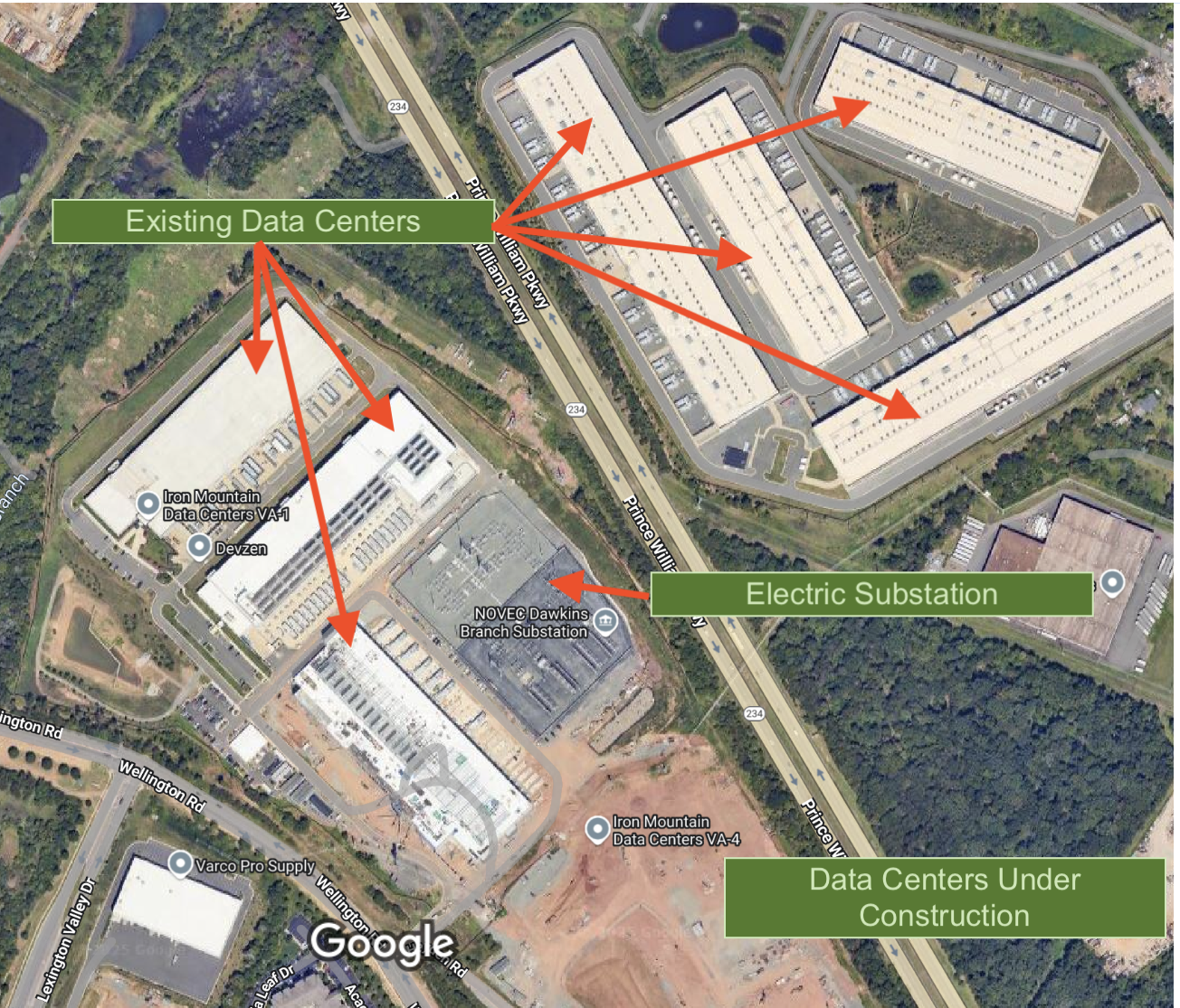
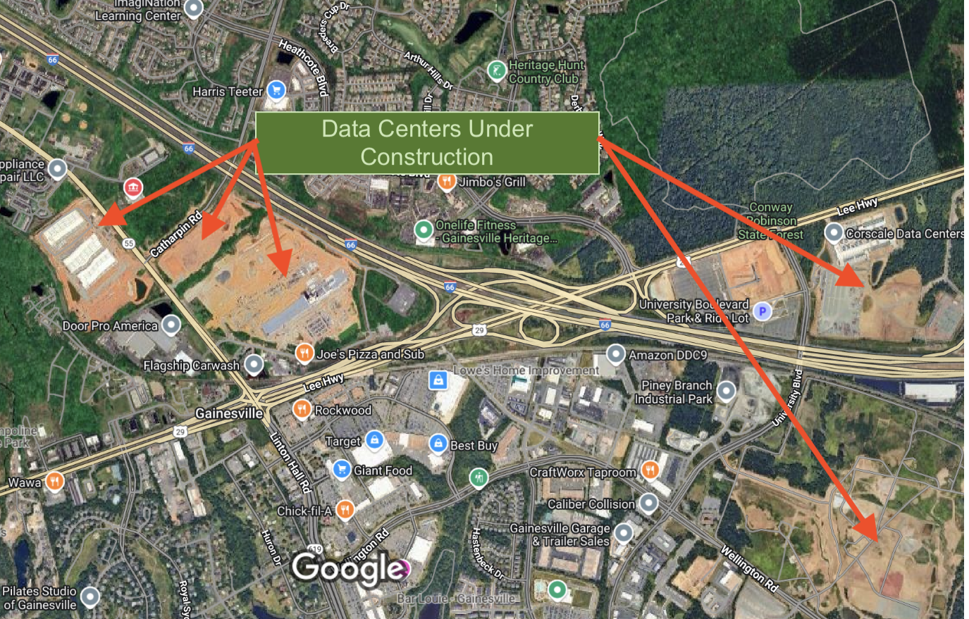
They tend to require lots of input data and many calculations so their development has expanded greatly in the last few years given the large increases in available data and affordable computing power (Figure 11.2).

They tend to require lots of input data and many calculations so their development has expanded greatly in the last few years given the large increases in available data and affordable computing power.

(a) Just a few of the many existing data centers in Northern Virginia, USA in 2025. Note the dedicated electrical power substation.

(b) Just a few of the many data centers under construction in Northern Virginia, USA in 2025.

Figure 11.2: Evidence of the growing demand for data centers to support machine learning and AI.

Note

Deep Learning and Neural Nets have evolved in both computing and statistical domains and combine aspects of networks and statistical methods and transformations. Thus they tend to use different terms describing the same concepts, e.g., “features” are “predictors” are “inputs.”

11.1 A Single-Layer Neural Network

Neural networks are still trying to estimate the true but unknown function that defines the relationship between one set of data and another.

• In the case of supervised learning, the relationship is between at set of input “features” (variables) \(X = X_1, \ldots, X_n\), the inputs, and a \(Y\) the response or output.

The goal is to approximate the true but unknown function that maps \(X \mapsto Y\) as accurately as possible.

One way to do this is through a neural network, which builds this relationship by passing inputs through one or more layers of intermediate computations, ultimately producing a predicted output.

• Similar to boosted trees, the layers may have multiple nodes where each node is “weak”, but the combination of of multiple nodes in the layer can generate “strong” (useful) results.

Figure 11.3 depicts a single layer neural network with

• input nodes on the left, one for each predictor \(X_1, X_2, X_3,\) and \(X_4\)
• a single “hidden” layer with multiple “units” (nodes), and
• an output layer on the right which generates the final prediction \(\hat{Y}\).

Figure 11.3: Single-layer neural network (ISLR2 Fig. 10.1): four input nodes \(X_1\)–\(X_4\) (left) feed into \(K\) hidden units in one hidden layer (centre), each computing a weighted sum passed through a non-linear activation function \(g(\cdot)\); the hidden-unit activations \(A_1\)–\(A_K\) are then combined by output weights \(\beta_k\) to produce the single prediction \(\hat{f}(X)\) (right).

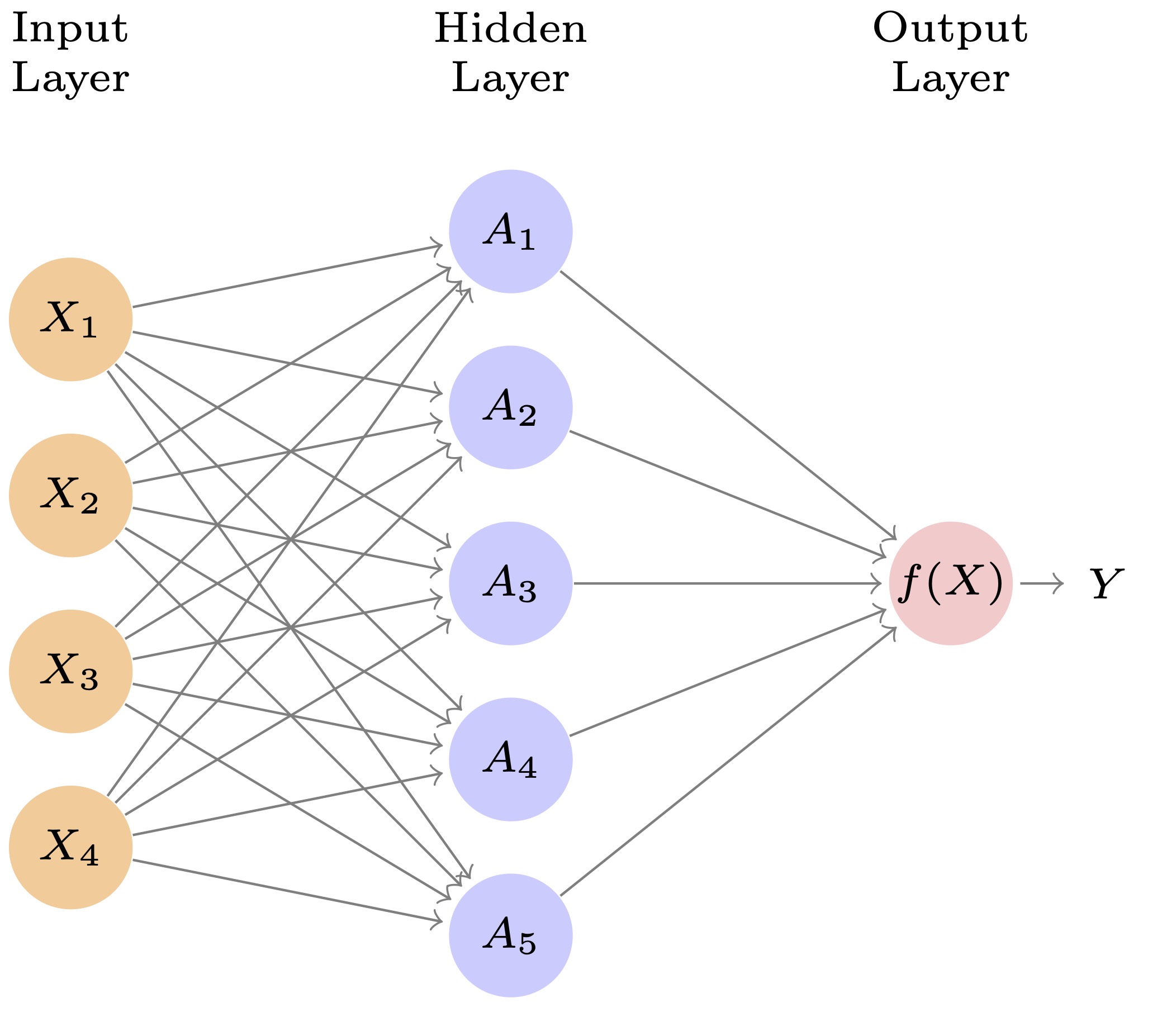
This network is taking information from four (predictor) inputs, \(X_1, X_2, X_3, X_4\) to generate an output layer \(\hat{f}(X)\) which predicts the response \(\hat{Y}\).

• The arrows from the inputs to the units (nodes) in the middle layer indicate where each input is fed to a middle layer unit that will then combine all the inputs it receives.
  • The number of units in a hidden layer, \(K\), is a tuning parameter (to be discussed later).
• In this single-layer model, each of the \(K\) hidden units makes its calculation and feeds its output to the output layer.
• The output layer then combines all of those \(K\) inputs to calculate the final result/prediction.

Note

The terms units, nodes, or “perceptrons” all refer to the individual elements of a network layer.

11.1.1 Structure of a Single Layer Neural Net

What distinguishes a neural network from other methods is the way the hidden layers make calculations on the inputs and the final layer then combines the outputs from the previous layer, (inputs to the final layer), to calculate a final prediction.

To understand what happens inside a neural network, it helps to think in terms familiar from linear regression.

• In a basic linear regression, we model:

\[Y = \beta_0 + \beta_1 X_1 + \beta_2 X_2 + \dots + \beta_p X_p + \varepsilon \tag{11.1}\]

or, using the \(\sum\) symbol

\[Y = \beta_0 + \sum_i\beta_iX_i \tag{11.2}\]

To put Equation 11.1 and Equation 11.2 in the context of neural networks,

• The coefficients \(\beta_j\) are “weights” that indicate how important each feature is to predicting \(Y\).
• The intercept \(\beta_0\) acts like a constant shift — a baseline level when all \(X_j = 0\)..

Neural networks use similar ideas but in layers.

In the hidden layer, each unit computes a weighted sum of its inputs plus a bias, and then applies a non-linear activation function \(g(\cdot)\):

• Let \(A_k\) represent the output, \(h_k(X)\), of the \(k\)^th unit in the hidden layer. Since this is a Neural Network equation we will use \(w_i\) instead of \(\beta_i\) for the “weights” and the bias term.

\(A_k\) is calculated by calculating the linear combination and then using the Activation function on it (right to left) in Equation 11.3.

\[A_k = h_k(X) = g(z) = g(w_0 + \sum_{j=1}^p w_jX_j). \tag{11.3}\]

where \(j = 1, \ldots, p\) indexes the input features and \(k\) indexes the hidden node. In the worked example this is written as \(z_{k,i} = w_{k,0} + \sum_{j=1}^p w_{k,j} X_{j,i}\) (Equation 11.23), adding the observation index \(i\) explicitly.

where

• \(X_j\) is the \(j\)^th input feature (for \(j = 1, \ldots, p\)),
• \(w_{kj}\) is the weight connecting input feature \(X_j\) to hidden unit \(k\),
• \(w_{k0}\) is the bias term for hidden unit \(k\),
• \(g(\cdot)\) is a nonlinear activation function (e.g., ReLU, sigmoid, tanh),
• \(z_k\) is just shorthand for the linear combination (before activation) for unit \(k\).
• \(h_k(X)\) just serves as a reminder that the output is really just a non-liner function of the inputs \(X\) for the node \(k\).

These \(w\)’s and biases \(w_{k0}\) play the same role as \(\beta\)’s in regression: they determine how much influence each input has, but for each hidden unit individually.

Analogy: You can think of the \(w_{kj}\) as being like regression coefficients, and the bias \(w_{k0}\) as the intercept for each mini-model inside the hidden layer.

The hidden unit output \(A_k\) is then passed to the output layer, which again uses its own weighted linear combination of the transformed inputs to create a prediction.

• Now in neural networks, it is customary to use \(\beta\)s again for the output layer since it a linear function, in a way representing the entire neural network as one huge function mimicking the true but unknown \(f(X)\).

\[f(X) = \beta_0 + \sum_{i=1}^K \beta_k A_k = \beta_0 + \sum_{i=1}^K \beta_k\, g\left(w_{k0} + \sum_{j=1}^p w_{kj}X_j\right). \tag{11.4}\]

Where

• \(\beta_k\) is the output layer weight for hidden unit \(k\)’s \(A_k\) A,
• \(\beta_0\) is the output bias term.

So in total:

• The first layer computes non-linear transformations of weighted combinations of inputs,
• The final layer is a linear model using those transformations as features.

11.1.2 Role of the Bias

Bias terms, both \(w_{k0}\) in the hidden layers and \(\beta_0\) in the output layer, help shift the activation threshold of each unit.

• If we left them out, every transformation would be forced to pass through the origin, which limits model flexibility just like in linear regression.

In fact, you can think of the bias \(w_{k0}\) as setting a threshold (like in animal neurons): it helps determine whether a unit “activates” or not.

• For example, if you’re using a sigmoid activation, the bias controls the input value where the sigmoid flips from low to high.

11.1.3 Activation Functions

The activation function \(g(\cdot)\) introduces non-linearity which is crucial for neural networks to allow for flexible non-linear relationships and interactions among the data.

• If you removed all activation functions (or used a linear one), the network would collapse into a linear model, no more powerful than standard regression.
  • Equation 11.4 would just be a linear combination of linear combinations from Equation 11.3 which is not new.

The user pre-selects the activation function with the goal of helping to clearly differentiate between signal and noise in the data.

An early choice was the sigmoid activation function

\[g(z) = \frac{e^z}{1+e^z} = \frac{1}{1+e^{-z}}. \tag{11.5}\]

• This is the same function we used with logistic regression.
• It has the nice property of transforming linear functions into probabilities from 0 to 1.
• Its sigmoid shape also helps highlight differences between signal and noise.

A more popular choice now is the ReLU (rectified linear unit) activation function.

\[g(z) = (z)_+ = \cases{0 \quad \text{if } z<0 \\ z\quad \text{otherwise}} \tag{11.6}\]

• The ReLU calculations can be stored and computed faster than the sigmoid calculations.
• By design, it encourages “sparse” activation (many values are zero), which can help reduce overfitting and improve generalization.

Figure 11.4 shows the non-linear shapes of a sigmoid and a ReLU activation function.

Figure 11.4: Sigmoid and ReLU activation functions (ISLR2 Fig. 10.2). Left: the sigmoid \(g(z)=1/(1+e^{-z})\) produces an S-shaped curve bounded between 0 and 1, saturating near \(\pm 1\) for large \(|z|\). Right: ReLU \(g(z)=\max(0,z)\) is exactly zero for \(z\leq 0\) and linear for \(z>0\), introducing sparsity and avoiding the vanishing-gradient problem that affects the sigmoid in deep networks.

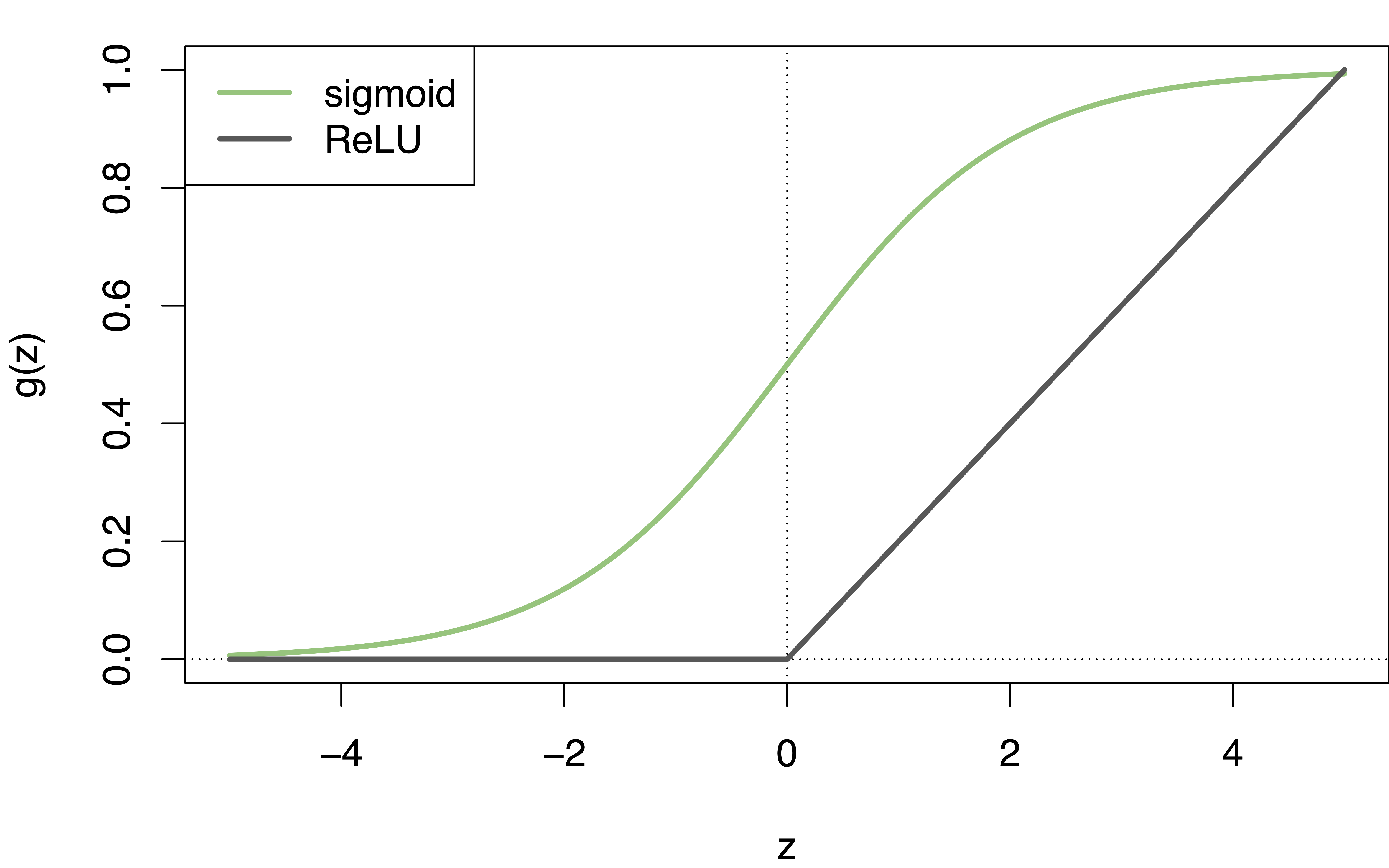
Activation functions are non-linear by choice to allow for non-linear relationships and interactions among the data.

• If the activation functions were linear, Equation 11.4 would just be a linear combination of linear combinations from Equation 11.3 which is not new.

However, even though the \(g(z)\) are non-linear, the combinations in Equation 11.4 are still linear in the inputs.

• The final model results from calculating linear combinations at each hidden unit, doing a non-linear transformation of each, and then, doing a linear combination on the transformed results.
• Since the final layer (Output) is still linear in its (transformed) inputs, we can use (for quantitative variables), the usual squared error loss (from linear regression) as an objective function (the loss function) to be minimized to calculate the \(\beta\)s, i.e..,

\[\sum_{i=1}^{n}(y_i - f(x_i))^2. \tag{11.7}\]

11.1.4 Learning the Weights and Biases

All of the weights \(w_{kj}\), biases \(w_{k0}\), and output weights \(\beta_k\) and \(\beta_0\) are “learned” from data.

Training typically involves defining a “loss function” for the output layer, e.g., squared error:

\[\sum_{i=1}^{n} \left( y_i - f(x_i) \right)^2 \tag{11.8}\]

Then using gradient descent and backpropagation to adjust the weights and biases to minimize this loss.

Tip 11.1: Choosing an Initial Network Architecture

There is no theorem that specifies the optimal number of hidden layers or nodes per layer for a given dataset. - Architecture selection is a hyperparameter decision governed by the same bias–variance tradeoff that applies to choosing \(k\) in KNN or the degree of a polynomial. - The workflow is: start with a reasonable architecture based on the heuristics in Table 11.1, fit the model, diagnose train vs. validation performance, then adjust the architecture if required.

Heuristics for Initial Architectures

Table 11.1: Initial architecture design heuristics.

Design decision	Starting guidance	Rationale
Number of hidden layers	1–2 for tabular data; add layers only when simpler model plateaus	Each layer learns more abstract features; most tabular problems do not need more than 2 dense layers
Nodes per layer	Between \(p\) and \(2p\) inputs; funnel shape (wider first layer, narrower second)	Enough capacity to learn patterns without diluting gradient signal; funnel compresses to relevant features
Total parameters	Aim for fewer than \(n/5\) free parameters as a rough ceiling	More parameters than this relative to \(n\) almost guarantees overfitting without heavy regularization
Output layer	1 node (regression); \(M\) nodes (classification)	Fixed by the problem — not a tuning decision

Other factors to consider:

• Data messiness / noise level: Noisier data favors shallower, more regularized networks. Deep networks fit noise aggressively and require stronger regularization to compensate.
• Number of input features \(p\): More inputs allow more nodes per layer before the parameter ceiling is reached.
• Nature of the inputs: Image, text, and sequence data benefit from specialized architectures (CNNs, RNNs, Transformers). Tabular/structured data generally does not.
• Computational budget: Deeper and wider networks cost more per epoch and typically require more epochs to converge.
• Symmetry-breaking at initialization: Always initialize weights randomly — see Equation 11.22 in the worked example. Identical initial weights mean all nodes in a layer compute the same thing and the layer collapses to a single effective node.

The typical answer: start simple (1 hidden layer, \(K \approx p\) nodes), check the train/validation gap, and grow or regularize from there. The tuning workflow in Section 11.8 provides a systematic approach.

11.2 Multi-layer Neural Networks

A single layer network can represent many possible \(\hat{f}(x)\).

Adding more hidden units in a layer and adding more layers allows for more possible transformations and provides more flexibility in the model.

• In general, adding more, smaller layers can make solutions easier to find than just adding more units in a single layer.

Figure 11.5 shows a multi-layer network for classifying digits (0-9) with a different number of units in each hidden layer.

• This network could used the MNIST Dataset of images of hand-written numbers as inputs to classify each image as a number.

Figure 11.5: Multi-layer neural network for digit classification (ISLR2 Fig. 10.4). The input layer receives the 784 pixel values of a \(28\times 28\) greyscale image. Hidden Layer 1 (\(K_1=256\) units) and Hidden Layer 2 (\(K_2=128\) units) learn progressively more abstract features; the output layer has \(M=10\) softmax units, one per digit class (0–9), producing class probabilities that sum to 1.

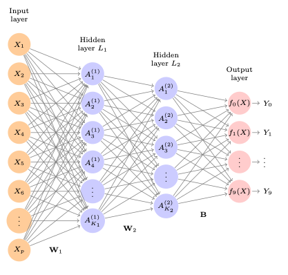
• It has two hidden layers L1 (256 units) and L2 (128 units).
• There are 10 nodes in the output layer since there are 10 possible levels to be classified
• Each is a dummy variable. In this case, the ten variables really represent a single qualitative variable so are dependent on each other.

Note

Each of the activations in the units in the second layer is still a function of the original input \(X\), albeit a transformed version of it based on the activations in the first layer.

Adding more and more layers to the model builds a series of simple transformations into a complex model for the final result.

With more layers comes more notation.

• We can add a superscript to indicate the layer, e.g., \(A^{(1)}_{k}\).
• Consider all the parameters for each layer as a matrix. Thus we have \(W_1\), \(W_2\) and \(B\) as our three matrices of “weights” for the network.

11.2.1 Coefficients to be Estimated

There are a lot of coefficients (weights) to be estimated in \(W_1\), \(W_2\), and \(B\).

There are 784 pixels in a \(28 \times 28\) pixel image. These are the inputs.

• Matrix \(W_1\) has \(785 \times 256 = 200,960\) elements. This is based on the 256 units and the 784 input values plus the intercept term (in NN called the “bias” term).
• Matrix \(W_2\) thus has \(128 \times 257 = 32,896\) (256 + bias term).
• Matrix \(B\) thus has \(10 \times 129 = 1,290\) elements. The 10 linear models for each level and the 128 outputs plus the bias term.

Together there are \(200,960 + 32,896 + 1,290 = 235,146\) coefficients (weights) to be estimated.

• This is 33 times more than just doing multinomial logistic regression.
• With a training set of only 60,000 images, there is a lot of opportunity for overfitting.

To avoid overfitting, some regularization is needed. Options include Ridge, Lasso, or neural-network specific methods such as dropout regularization.

11.2.2 Softmax Activation Function

Since the outputs are dependent, they represent the probabilities that a given input corresponds to each possible image class and must sum to 1, this model will use the softmax activation function for the output layer.

\[f_m(X) = Pr(Y=m | X) = \frac{e^{Z_m}}{\sum_{l=0}^{9}e^{Z_l}} \tag{11.9}\]

Equation 11.9 is a generalization of the logistic function from binary logistics regression to multiple levels needed in multinomial logistic regression.

• Note: the sum runs from \(l = 0\) to \(9\) here because the MNIST example has 10 classes (digits 0–9).
• In the general case, with \(M\) classes, the sum runs from \(l = 1\) to \(M\), as used in the worked example (Equation 11.9 in the worked example section).

During each forward pass, the model assigns probabilities to each possible output. This is the result of the softmax “soft” prediction instead of choosing just the one value with the highest probability.

• These output probabilities are a vector that sums to 1. One class may have the highest probability, but most probabilities are typically nonzero.
• When training starts, probabilities are fairly evenly distributed given the random assignment of initials weights and biases. As training proceeds through multiple epochs, the model gradually shifts increases the probability for the “correct” output value and decreases other probabilities.
• A key advantage of softmax is that Equation 11.9 is differentiable, which allows us to compute gradients to feed backpropagation. In contrast, the “hard” max() function is not differentiable and therefore not suitable during training.

After training is complete, when we no longer need gradients, we can apply a max() operation to the softmax output vector to make a final “hard” prediction, selecting the class (dummy variable) with the highest predicted probability as our prediction.

11.2.3 Minimization by Cross-Entropy

Since the response in this setting is qualitative (i.e., a categorical class label), we minimize the negative multinomial log-likelihood, commonly referred to as [cross-entropy loss](https://en.wikipedia.org/wiki/Cross-entropy.

When class labels are represented directly as integer indices (e.g., \(y_i \in \{0, 1, \ldots, 9\}\)), the cross-entropy loss, for all \(n\) inputs, takes the form:

\[R(\theta) = -\sum_{i=1}^{n} \log(f_{y_i}(x_i)) \tag{11.10}\]

• Here, \(y_i\) is the index of the true class label for the \(i^\text{th}\) input.
• \(f_{y_i}(x_i)\) is the predicted probability (from the softmax output in Equation 11.9) corresponding to that true class.

This form is computationally efficient and is the one typically used in practical implementations.

Alternatively, theoretical discussions may express cross-entropy using “one-hot encoding” of the target vector:

\[R(\theta) = -\sum_{i=1}^{n}\sum_{m=0}^{9} y_{im} \log(f_m(x_i)) \tag{11.11}\]

• Here, \(y_{im} = 1\) if class \(m\) is the correct label for input \(i\), and 0 otherwise.
• \(f_m(x_i)\) is the predicted probability for class \(m\).

Equation 11.11 is mathematically equivalent to Equation 11.10 when \(y_{im}\) is one-hot encoded, and is often used to conceptually explain cross-entropy as a comparison between two distributions.

Entropy (from information theory) measures the amount of “uncertainty” or “surprise” in a probability distribution. For a predicted distribution \(p=f(X_i)\) (from our softmax output), the entropy is:

\[H(p) = -\sum_{m=0}^9 p_m \log(p_m) \tag{11.12}\]

• A nearly uniform prediction (e.g., \([0.1, 0.1, ..., 0.1]\)) has high entropy (like at the end of the first epoch of training).
• A perfectly confident prediction (e.g., \([0, 0, 1, 0, ..., 0]\)) has low entropy.
• After the selected number of epochs, the entropy in the predicted distribution should be lower than when it started as the probabilities increase for the more-correct values and decrease for others.

Cross-entropy compares two distributions:

• The true distribution \(y_i\) and
• The predicted distribution \(f(x_i)\).

It is defined as:

\[H(y_i, f(x_i)) = -\sum_{m} y_{im} \log(f_m(x_i)) \tag{11.13}\]

• When \(y_{im}\) is a one-hot vector, this reduces to just \(-\log(f_{m}(x_i))\), where \(m\) is the true class.
• In practice, the indexed form of the loss (as in Equation 11.10) is used because it’s faster and avoids explicit one-hot encoding which takes time and memory with all the 0s.

Cross-entropy is useful in conjunction with Softmax as it is an efficient way to penalize the model more heavily when it assigns a low probability to the true class.

11.3 Fitting a Neural Network

Fitting a neural network is complex due to the necessary use of non-linear activation functions.

Warning

Deep learning and neural networks is an active area of research across many communities. You will see many different terms often describing the same concept or approach.

• You will also see many articles or references describing the latest approaches.

What follows is not exhaustive by any means. It is designed to provide familiarity with some approaches to provide a basic understanding.

• There are many tuning (hyper-parameters) in neural networks and the selection for a given set of data is still very much an art more than a science.

While the objective function in Equation 11.7 looks familiar, minimizing it over the activations functions is non-linear.

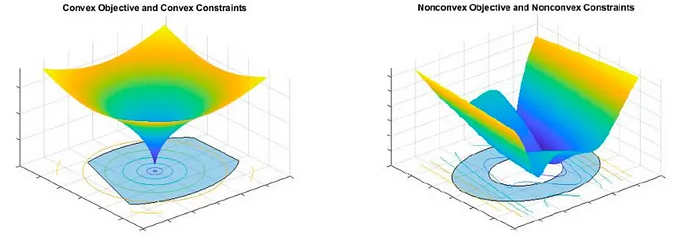
Important

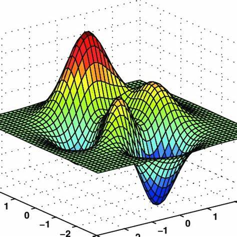
Neural Networks use non-linear activation functions so their objective functions are non-convex and have multiple local optima in addition to a global optimum.

Instead of trying to find the “best” model at the one global optimum, potentially out of millions, we seek to find a useful model at a “reasonable” local minima.

(a) Left panel: a convex bowl-shaped loss surface with a single global minimum that gradient descent always reaches regardless of starting point. Right panel: a non-convex surface with both a shallow local minimum and a deeper global minimum — gradient descent may converge to either depending on initialization and learning rate.

(b) A hand-drawn 2-D illustration of a non-convex loss curve with a shallow local minimum on the left and a deeper global minimum on the right, showing how gradient descent starting from different positions can terminate at different optima.

(c) A non-convex loss surface with multiple local optima and saddle points (Kanwal et al. (2013)). Gradient descent started at different initial parameter values (different starting positions on the surface) can converge to different local minima, none of which need be the global minimum. This is a key practical challenge in training deep neural networks.

Figure 11.6: Representations of convex and non-convex loss surfaces — Figure 11.6 illustrates a convex bowl (single global minimum), a simple hand-drawn non-convex curve, and a research example with multiple local optima.

Two strategies help find better local optima and reduce the chance of overfitting.

• Slow Learning: As we saw with boosting, slow learning, small steps in gradient descent helps reduce the chance of overfitting. The algorithm stops when overfitting is detected.
• Regularization: Imposing penalties on the parameters such as we saw with Ridge and Lasso regression.

Assume all the parameters (coefficients) are in a single vector \(\theta\).

Define the objective function for \(R(\theta)\) as

\[R(\theta) = \frac{1}{2}\sum_{i=1}^n(y_i - f_\theta(x_i))^2. \tag{11.14}\]

To find the best parameters \(\theta\) for our model, we want to minimize the objective function \(R(\theta)\).

A general algorithm to minimize Equation 11.14 could be:

1. Initialize: Make an initial guess for all the parameters, \(\theta^0\), and set \(t = 0.\)
2. Update step: Find a vector \(\delta\) that represents a small change in \(\theta\)such that the new parameters \(\theta^{t+1} = \theta^t + \delta\) reduce the value of \(R(\theta^t)\).
3. Check improvement: If \(R(\theta^{t+1}) < R(\theta^t)\), set \(t = t + 1\) and return to step 2.
4. Stop condition: If no meaningful reduction is achieved, stop. The algorithm has likely reached a local minimum of the loss function.

So how to find a good \(\delta\)?

11.3.1 Gradient Descent and Backpropagation

Finding \(\delta\) is key in neural network optimization.

• We want to adjust the vector \(\theta\) in the direction that reduces the error most efficiently.
• That direction is given by the negative of the gradient of the objective function: \(\delta = -\eta \cdot \nabla_\theta R(\theta)\).

Note

Think of the gradient as a slope of a line but in multiple dimensions, the default calculation points in the direction of steepest increase in the loss.

So, to minimize the loss, we move in the opposite direction of the gradient, the negative gradient.

Imagine you are on a hill and want to get to the valley below (reach the lowest point (the minimum loss)).

• The gradient is the direction the hill is steepest.
• If you step in the opposite direction of the gradient, you’re going downhill and finding the better set of weights and bias that will give you a lower error.
• The learning rate is how big of a step you take before you calculate the next gradient.

Each weight and bias has its own gradient; we can update them individually using a method called gradient descent.

• The gradient, \(\nabla_\theta R(\theta)\), shows how the error would change by updating (increasing or decreasing) each weight/bias.
• The learning rate, \(\eta\) (eta) controls how big a step we take in the opposite direction of the gradient.
• The minus sign ensures we move in the direction that reduces the error, not increases it.
• You may see the term the “gradient vector” for a node which is shorthand for the set of all the individual gradient entries for each weight/bias parameter combined into a vector.

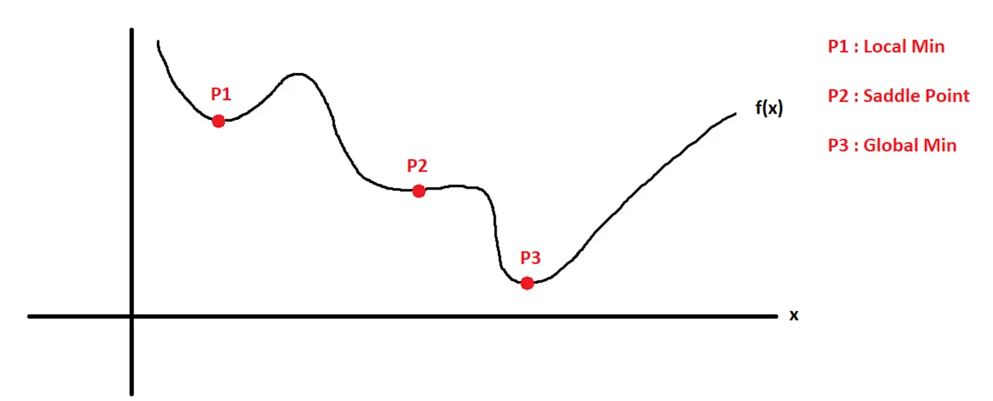
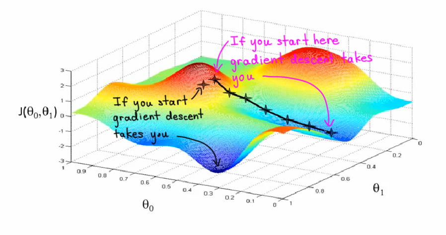
Figure 11.7 provides one view of how gradient descent can lead to different local optima with slightly different starting points.

Figure 11.7: Conceptual illustration of gradient descent on a non-convex loss surface (Rashida048 (2020)). Two trajectories are shown starting from slightly different initial parameter values: one descends into a shallow local minimum while the other reaches the deeper global minimum, demonstrating the sensitivity of gradient descent to initialization — the motivation for Xavier initialization (Equation 11.22) and random restarts.

Let’s define the value of the gradient of \(R(\theta)\) evaluated at its current value \(\theta^m\) as the vector of its partial derivative evaluated at \(\theta^m\):

\[\nabla R(\theta^{m})= \frac{\partial R(\theta)}{\partial \theta}\biggr\rvert_{\theta=\theta^m}. \tag{11.15}\]

• This gives the direction to move in \(\theta\) space in which \(R(\theta)\) increases the most rapidly.

We want to move in the opposite direction. So we update \(\theta^{m+1}\) as

\[\theta^{m+1} \leftarrow \theta^{m} - \rho \nabla R(\theta^{m}). \tag{11.16}\]

• where \(\rho\) is a learning parameter that controls the “rate of learning”.
• For very small \(\rho\) this should decrease \(R(\theta)\) such that we don’t go too far past \(R(\theta)=0\).

The good news is that Equation 11.14 is a set of sums so Equation 11.15 is also a set of sums.

Expanding the \(f_\theta(x_i)\) term in Equation 11.14, we get the complicated looking expression for a single observation \(i\)

\[R_i(\theta) = \frac{1}{2}\left(y_i - \beta_o - \sum_{k=1}^K\beta_k\,g(w_o + \sum_{j=1}^{p}w_{kj}x_{ij})\right)^2. \tag{11.17}\]

Let’s define

\[z_{ik} = w_{k0} + \sum_{j=1}^pw_{kj}x_{ij} \tag{11.18}\]

where the subscript order is \((\text{obs}, \text{node})\): \(i\) is the observation, \(k\) is the hidden node.

• Note: in Section 11.4, this same quantity is written \(z_{k,i}\) (Equation 11.23) with node index first and comma-separated; both forms are common as the two forms are identical.

We can use \(z_{ik}\) to simplify Equation 11.17 as

\[R_i(\theta) = \frac{1}{2}\left(y_i - \beta_o - \sum_{k=1}^K\beta_k\,g(z_{ik})\right)^2. \tag{11.19}\]

Since \(\delta\) is the change we want in the current values of \(\theta\), let’s take the partial derivative of Equation 11.19 with respect to \(\beta_k\) (using the chain rule) to find a good value of \(\delta\) for the \(\beta\)s in the output layer as

\[\begin{align} \frac{\partial R_i(\theta)}{\partial\beta_k} &= \frac{\partial R_i(\theta)}{\partial f_\theta(x_i)} . \frac{\partial f_\theta(x_i)}{\partial\beta_k} \\ &= -(y_i - f_\theta(x_i)) . g(z_{ik}) \end{align} \tag{11.20}\]

where we are using the derivative of Equation 11.14 to get the first term.

To find a value of \(\delta\) for the \(w\)’s in the hidden layer, we can now take the derivative of Equation 11.19 with respect to \(w_{kj}\) to get

\[\begin{align} \frac{\partial R_i(\theta)}{\partial w_{kj}} &= \frac{\partial R_i(\theta)}{\partial f_\theta(x_i)}\,\, .\,\, \frac{\partial f_\theta(x_i)}{\partial g(z_{ik})} \quad . \quad \frac{\partial g(z_{ik})}{\partial z_{ik}} . \frac{\partial z_{ik}}{\partial w_{kj}}\\ &= -(y_i - f_\theta(x_i))\,\, .\,\, \beta_k \,\,.\,\, g'(z_{ik}).x_{ij} \end{align} \tag{11.21}\]

where we are using the derivative of Equation 11.14 for the first term, the derivative of Equation 11.4 for the second term, the derivative of \(g(z)\) for the third, and the derivative of Equation 11.18 for the fourth term.

Important

The first term in both partial derivatives is the residual from the final layer \((y_i - f_\theta(x_i))\).

Equation 11.20 shows the \(\delta_\beta\)’s are based on how the residual gets allocated across each of \(K\) hidden units in the last hidden layer given the value of \(g(z_{ik})\) for that unit.

• Note that \(g(z_{ik}) \equiv A_k\), the activation output, so this is the same two-factor product derived in detail in the worked example as Equation 11.39.

Equation 11.21 shows the \(\delta_w\)’s are based on how the residual gets allocated across each of \(j\) inputs to the unit according to the value of each hidden unit’s \(\beta_k g'(z_{ik})\) for each \(x_i\).

• The form of \(g'()\) will depend upon the activation function we chose.
• This is the single-hidden-layer case; in a two-hidden-layer network the input \(x_{ij}\) is replaced by the previous layer’s activation \(A^{(1)}_{j,i}\) (see Equation 11.41 and Equation 11.43 in the worked example for the full derivation).

By starting with the final residual, we can now use the derivatives to calculate the new \(\delta\) for each parameter in each layer by moving from right to left across the network.

This process is known as backpropagation, as we are moving backwards, (right to left) to propagate (pass on) the information from the latest residuals to update the weights (coefficients/parameters) for each unit/node in each layer.

11.3.1.1 Backpropagation: An Intuitive Analogy

Backpropagation is how a neural network learns from its mistakes. You can think of it like how a child learns to shoot a basketball:

1. Take a shot: The child throws the ball; this is the network making a prediction.
2. See the result: The child sees if the shot missed or scored; this is the model calculating the error.
3. Figure out what went wrong: Did the shot go too far? Was the angle off?; this is feedback.
4. Adjust next time: The child throws again, tweaking their motion; this is weight adjustment using backpropagation.

How It Works in a Neural Network

• The prediction is the forward pass: the model computes \(f_\theta(x)\).
• The error is the difference between predicted and actual values: \(y_i - f_\theta(x_i)\).
• Backpropagation takes this final error and sends it backward through the network, using the chain rule as it goes layer by layer, to calculate the gradient of the loss with respect to every weight/bias parameter.

In other words:

Starting with the residual (final error), we compute how much each parameter contributed to that error and how it should change.

This is done layer-by-layer from right to left (going backwards, output to input), updating weights across each layer.

11.3.1.2 Why It Matters

Backpropagation makes training deep models computationally feasible. It allows the model to:

• Efficiently compute \(\nabla_\theta R(\theta)\) for all parameters, even in deep networks.
• Update its parameters using a simple rule: \(\theta^{t+1} = \theta^t - \eta \cdot \nabla_\theta R(\theta^t)\)
• Learn from experience, gradually reducing error as it sees more examples.

11.3.2 Epochs

We know how to do three things:

1. A Forward Pass: Use the initial inputs to compute the outputs for each unit in each layer (using the estimated weights and activation functions) to get to an output layer where the parameters (\(\beta\)s) are estimated (based on optimizing a loss function) to produce a prediction \(\hat{y}_i\) for each observation \(x_i\).
2. Calculate the residuals \((\hat{y}_i - y_i)\).
3. A Backwards Pass: Use the gradient of the loss function to allocate the residuals as a \(\delta\) to update each of the weights in the network thorough backpropagation.

We will repeat those steps multiple times in training the network.

An Epoch is defined as one complete forward pass and a complete backward pass (steps 1-3) through the network where every observation in the training data set contributes to the update.

• The number of epochs to use is a tuning parameter when building the model.
• There are trade-offs of time and accuracy as well preventing overfitting.

11.4 Worked Example of Training a Neural Network

This section walks through the numerical calculations that occur inside a neural network during training, node by node and layer by layer.

The same network architecture is used throughout, with the exception of the output layer which has one node for the regression problem and two nodes for the classification problem.

• This means every equation can be traced from raw inputs through the forward pass to the output layer and then through backpropagation where parameters get updated in each layer.

The Network architecture is depicted in Figure 11.8.

• 10 observations in the training batch
• 5 input nodes (\(X_1, X_2, X_3, X_4, X_5\))
• 2 hidden layers (Hidden Layer 1 with \(K_1 = 4\) units; Hidden Layer 2 with \(K_2 = 3\) units)
• 1 output node (regression: movie attendance) or 2 output nodes (classification: Hit or Flop)

%%{init: {"theme": "base", "themeVariables": {"clusterBkg": "transparent", "clusterBorder": "none", "edgeLabelBackground": "transparent", "lineColor": "#222222"}}}%%
flowchart LR
    subgraph INPUT["Input Layer<br/>(5 nodes, 10 obs)"]
        X1(["X₁"])
        X2(["X₂"])
        X3(["X₃"])
        X4(["X₄"])
        X5(["X₅"])
    end

    subgraph H1["Hidden Layer 1<br/>(K₁ = 4 nodes)"]
        A11(["A₁⁽¹⁾"])
        A12(["A₂⁽¹⁾"])
        A13(["A₃⁽¹⁾"])
        A14(["A₄⁽¹⁾"])
    end

    subgraph H2["Hidden Layer 2<br/>(K₂ = 3 nodes)"]
        A21(["A₁⁽²⁾"])
        A22(["A₂⁽²⁾"])
        A23(["A₃⁽²⁾"])
    end

    subgraph OUT_R["Output Layer<br/>(Regression)"]
        YR(["ŷ<br/>Attendance"])
    end

    subgraph OUT_C["Output Layer<br/>(Classification)"]
        YC1(["P̂(Hit)"])
        YC2(["P̂(Flop)"])
    end

    %% Input → H1 (all-to-all)
    X1 --> A11 & A12 & A13 & A14
    X2 --> A11 & A12 & A13 & A14
    X3 --> A11 & A12 & A13 & A14
    X4 --> A11 & A12 & A13 & A14
    X5 --> A11 & A12 & A13 & A14

    %% H1 → H2 (all-to-all)
    A11 & A12 & A13 & A14 --> A21
    A11 & A12 & A13 & A14 --> A22
    A11 & A12 & A13 & A14 --> A23

    %% H2 → Output (regression)
    A21 & A22 & A23 --> YR

    %% H2 → Output (classification)
    A21 & A22 & A23 --> YC1
    A21 & A22 & A23 --> YC2

    %% Subgraph backgrounds — transparent so arrows are never covered
    style INPUT fill:transparent,stroke:none,color:#222222
    style H1    fill:transparent,stroke:none,color:#222222
    style H2    fill:transparent,stroke:none,color:#222222
    style OUT_R fill:transparent,stroke:none,color:#222222
    style OUT_C fill:transparent,stroke:none,color:#222222

    %% Node styling — light fills, dark text so readable on any background
    classDef input   fill:#4393c3,stroke:#2166ac,color:#ffffff,font-size:13px
    classDef hidden1 fill:#74add1,stroke:#4393c3,color:#ffffff,font-size:13px
    classDef hidden2 fill:#abd9e9,stroke:#74add1,color:#222222,font-size:13px
    classDef outreg  fill:#d6604d,stroke:#b2182b,color:#ffffff,font-size:13px
    classDef outclf  fill:#f4a582,stroke:#d6604d,color:#222222,font-size:13px

    class X1,X2,X3,X4,X5 input
    class A11,A12,A13,A14 hidden1
    class A21,A22,A23 hidden2
    class YR outreg
    class YC1,YC2 outclf

Figure 11.8: Neural network architecture for the worked example. Left to right: 5 input nodes, Hidden Layer 1 (K₁ = 4 nodes), Hidden Layer 2 (K₂ = 3 nodes), and the output layer (1 node for regression; 2 nodes for classification). Arrows represent weighted connections; every node in each layer connects to every node in the next layer (fully connected).

The next sections trace the calculations relevant to one node, node \(k = 1\) in Hidden Layer 1, through initialization, the forward pass, loss computation, and backpropagation.

11.4.1 Notation Reference

A neural network models requires lots of calculations so the notation used to different identify the elements of the model across multiple layers and types of calculations can get confusing.

• It does not help that different sources may use different symbology as well.

The tables below define every symbol and index used in the equations throughout this walkthrough to provide a ready reference for working through the steps.

• Careful attention to upper- vs. lower-case and to superscripts vs. subscripts can reduce confusion between “a quantity for node \(k\)” and “the total number of nodes \(K\).”

11.4.1.1 Indices

Table 11.2: Index symbols from Figure 11.8 which are used throughout the worked example.

Symbol	Meaning	Range in this example
\(i\)	Observation (row) index	\(i = 1, \ldots, n\); here \(n = 10\)
\(j\)	Input feature index	\(j = 1, \ldots, p\); here \(p = 5\)
\(k\)	Hidden unit (node) index in Layer 1	\(k = 1, \ldots, K_1\); here \(K_1 = 4\)
\(m\)	Hidden unit (node) index in Layer 2, or output class index	\(m = 1, \ldots, K_2\) (hidden) or \(m = 1, \ldots, M\) (output classes); here \(K_2 = 3\), \(M = 2\)
\(l\)	Summation index over output classes (used inside Softmax only)	\(l = 1, \ldots, M\)
\(K_1\)	Total number of nodes in Hidden Layer 1	4 (fixed for this example)
\(K_2\)	Total number of nodes in Hidden Layer 2	3 (fixed for this example)
\(n\)	Total number of observations (training batch size)	10
\(p\)	Total number of input features	5
\(M\)	Total number of output classes (classification only)	2 (Hit, Flop)

11.4.1.2 Weights and Biases

Table 11.3: Weight and bias parameter symbols.

Symbol	Meaning	Dimensions
\(w_{k,j}\)	Weight connecting input \(X_j\) to hidden node \(k\) in Layer 1	one scalar per \((k, j)\) pair
\(w_{k,0}\)	Bias for hidden node \(k\) in Layer 1 (the intercept; no input multiplied)	one scalar per node \(k\)
\(w^{(2)}_{m,k}\)	Weight connecting Layer 1 node \(k\) to Layer 2 node \(m\); superscript \((2)\) denotes Layer 2	one scalar per \((m, k)\) pair
\(w^{(2)}_{m,0}\)	Bias for Layer 2 node \(m\)	one scalar per node \(m\)
\(\beta_k\)	Output layer weight connecting Layer 2 node \(k\) to the output (regression); or \(\beta_{m,k}\) for class \(m\) in classification	one scalar per \(k\) (regression) or per \((m, k)\) (classification)
\(\beta_0\)	Output layer bias (regression)	one scalar
\(\beta_{m,0}\)	Output layer bias for class \(m\) (classification)	one scalar per class \(m\)
\(\theta\)	Generic placeholder for any trainable parameter (\(w\) or \(\beta\))	—

11.4.1.3 Pre-activations and Activations

Table 11.4: Pre-activation and activation symbols.

Symbol	Meaning	Note
\(z_{k,i}\)	Pre-activation (linear combination) at Layer 1 node \(k\) for observation \(i\): \(w_{k,0} + \sum_j w_{k,j} X_{j,i}\)	Input to \(g(\cdot)\); sometimes written \(z^{(1)}_{k,i}\)
\(z^{(2)}_{m,i}\)	Pre-activation at Layer 2 node \(m\) for observation \(i\)	Superscript \((2)\) = Layer 2
\(Z_m\)	Pre-softmax score at output node \(m\) for classification: \(\beta_{m,0} + \sum_k \beta_{m,k} A^{(2)}_{k,i}\)	Notation matches ISLR2 Ch. 10
\(A_{k,i}\)	Activation (output) of Layer 1 node \(k\) for observation \(i\): \(A_{k,i} = g(z_{k,i})\)	Also written \(A^{(1)}_{k,i}\)
\(A^{(2)}_{m,i}\)	Activation of Layer 2 node \(m\) for observation \(i\): \(A^{(2)}_{m,i} = g(z^{(2)}_{m,i})\)	Input to the output layer
\(g(\cdot)\)	Activation function applied element-wise at each hidden node	e.g., ReLU, sigmoid, linear
\(g'(\cdot)\)	Derivative of the activation function (used in backpropagation)	ReLU: \(g'(z)=\mathbf{1}[z>0]\); sigmoid: \(g(z)(1-g(z))\)

11.4.1.4 Predictions and Loss

Table 11.5: Prediction and loss symbols.

Symbol	Meaning
\(\hat{y}_i\)	Predicted continuous output for observation \(i\) (regression)
\(y_i\)	True (observed) outcome for observation \(i\)
\(\hat{P}(m \mid x_i)\)	Predicted probability of class \(m\) for observation \(i\) (classification)
\(f_m(X)\)	Softmax probability for class \(m\): \(e^{Z_m} / \sum_l e^{Z_l}\)
\(\mathbf{1}[y_i = m]\)	Indicator function: equals 1 if the true class of observation \(i\) is \(m\), else 0
\(R(\theta)\)	Total training loss over all \(n\) observations (function of all current parameters \(\theta\))
\(\text{Loss}_i\)	Per-observation loss: \(\frac{1}{2}(y_i - \hat{y}_i)^2\) (regression) or \(-\log \hat{P}(y_i)\) (classification)

11.4.1.5 Training

Table 11.6: Training and optimization symbols.

Symbol	Meaning
\(\eta\)	Learning rate: step size for each gradient descent update (same as \(\rho\) in ISLR2)
\(\delta^{\text{out}}_{i}\)	Error signal at the output layer for observation \(i\) (regression: \(-(y_i - \hat{y}_i)\); classification: \(\hat{P}(m) - \mathbf{1}[y_i=m]\))
\(\frac{\partial R}{\partial \theta}\)	Partial derivative (gradient) of the total loss with respect to parameter \(\theta\)
\(\nabla_\theta R\)	Gradient vector of \(R\) with respect to all parameters

11.4.1.6 Key Distinction: Upper- vs. Lower-Case

Table 11.7: Key upper- vs. lower-case distinctions.

Pair	Upper case	Lower case
\(K_1\) vs. \(k\)	Total nodes in Layer 1 (an integer, e.g., 4)	Index of a specific node (1 to \(K_1\))
\(K_2\) vs. \(m\)	Total nodes in Layer 2 (e.g., 3)	Index of a specific node (1 to \(K_2\))
\(N\) / \(n\) vs. \(i\)	Total observations (e.g., 10)	Index of a specific observation
\(P\) / \(p\) vs. \(j\)	Total input features (e.g., 5)	Index of a specific input feature
\(M\) vs. \(m\)	Total output classes (e.g., 2)	Index of a specific class

11.4.2 Step 1: Initialization of the Neural Network Model’s Weights and Biases

Before training can begin, every weight \(w_{kj}\) and bias \(w_{k0}\) must be assigned an initial starting value.

• We cannot start at zero for all weights because that would make every hidden unit identical and no learning would occur (known as the symmetry problem (see Zhao et al. (2025))).

Convention: Choose values for weights and biases from a small random distribution.

• A common choice is the Xavier / Glorot initialization:

\[w_{kj} \sim \text{Uniform}\!\left(-\frac{1}{\sqrt{p}},\; \frac{1}{\sqrt{p}}\right) \tag{11.22}\]

where \(p\) is the number of inputs to the unit.

• With \(p = 5\) inputs, the range is \(\approx (-0.447,\; 0.447)\).

Our Example: Node \(k=1\) in Hidden Layer 1

The node receives inputs \(X_1, \ldots, X_5\). We randomly initialize (Table 11.8):

Table 11.8: Randomly initialized weights and bias for node \(k=1\), Layer 1.

Parameter	Symbol	Initialized Value
Bias	\(w_{1,0}\)	\(-0.12\)
Weight for \(X_1\)	\(w_{1,1}\)	\(+0.34\)
Weight for \(X_2\)	\(w_{1,2}\)	\(-0.21\)
Weight for \(X_3\)	\(w_{1,3}\)	\(+0.07\)
Weight for \(X_4\)	\(w_{1,4}\)	\(+0.41\)
Weight for \(X_5\)	\(w_{1,5}\)	\(-0.18\)

Similarly, every other node in Hidden Layer 1 and Hidden Layer 2 gets its own randomly initialized set of weights and biases.

The output layer weights \(\beta_0, \beta_1, \ldots, \beta_{K_2}\) are also randomly initialized.

What these parameters represent:

• \(w_{1,j}\): how much influence input \(X_j\) has on node 1’s activation.
• \(w_{1,0}\) (bias): a learnable baseline shift, like an intercept in regression.

Total parameters to initialize for this network (with \(K_1 = 4\) units in Layer 1 and \(K_2 = 3\) units in Layer 2):

• Hidden Layer 1: \(K_1 \times (p + 1) = 4 \times 6 = 24\) parameters
• Hidden Layer 2: \(K_2 \times (K_1 + 1) = 3 \times 5 = 15\) parameters
• Output layer: \(1 \times (K_2 + 1) = 4\) parameters (regression) or \(2 \times (K_2 + 1) = 8\) (classification)

All of these are set once at initialization and then updated iteratively during training.

11.4.3 Step 2: Forward Pass

We start with the First Hidden Layer Node

For observation \(i = 1\), the (possibly scaled) input values are in Table 11.9:

Table 11.9: Input feature values for observation \(i=1\).

Input	Value
\(X_1\)	\(1.5\)
\(X_2\)	\(0.8\)
\(X_3\)	\(-0.3\)
\(X_4\)	\(2.1\)
\(X_5\)	\(0.5\)

11.4.3.1 Step 2.1 Compute the Pre-activation Value

Compute the linear combination \(z\) using the node’s current bias and weights (Equation 11.23):

\[z_{k,i} = w_{k,0} + \sum_{j=1}^{p} w_{k,j} X_{j,i} \tag{11.23}\]

\[z_{1,1} = w_{1,0} + w_{1,1}X_1 + w_{1,2}X_2 + w_{1,3}X_3 + w_{1,4}X_4 + w_{1,5}X_5\]

\[z_{1,1} = (-0.12) + (0.34)(1.5) + (-0.21)(0.8) + (0.07)(-0.3) + (0.41)(2.1) + (-0.18)(0.5)\]

\[z_{1,1} = -0.12 + 0.51 - 0.168 - 0.021 + 0.861 - 0.09 = \mathbf{0.972}\]

This \(z\) value is the pre-activation, the weighted sum of inputs plus bias. It is the same computation as a linear regression prediction, but it is not the final output of this node.

11.4.3.2 Step 2.2 Apply the Activation Function** \(g(z)\):

Compute the node’s output (activation) value using (Equation 11.24):

\[A_{k,i} = g(z_{k,i}) \tag{11.24}\]

For node \(k=1\), observation \(i=1\): \(A_{1,1} = g(z_{1,1}) = g(0.972)\).

The choice of \(g(\cdot)\) determines the behavior of the node. Section 11.4.3.2.1 discusses some options.

11.4.3.2.1 Activation Functions at a Hidden Layer Node

The pre-activation value \(z_{1,1} = 0.972\) passes through an activation function. Here is what each of three common choices produces.

11.4.3.2.1.1 Option A - Linear Activation

\[g(z) = z \tag{11.25}\]

\[A_{1,1} = 0.972\]

Behavior: The output equals the input. No transformation occurs.

Problem: If every hidden unit uses a linear activation, the entire network collapses to a single linear model, thus no more expressive than ordinary linear regression.

• For this reason, linear activation is not used in hidden layers in practice.
• It is the default for the output node in regression problems.

11.4.3.2.1.2 Option B - Sigmoid Activation

\[g(z) = \frac{1}{1 + e^{-z}} \tag{11.26}\]

\[g(0.972) = \frac{1}{1 + e^{-0.972}}\]

\[A_{1,1} = \frac{1}{1 + 0.3786} = \frac{1}{1.3786} \approx \mathbf{0.725}\]

Behavior: Squashes any real number into the range \((0, 1)\).

• Large positive \(z\) → output near 1 (unit “fires strongly”)
• Large negative \(z\) → output near 0 (unit “suppressed”)
• \(z = 0\) → output = 0.5

Historical use: Sigmoid was the early standard activation. It mimics the biological neuron’s firing threshold.

Limitation: For very large or very small \(z\), the sigmoid is nearly flat with its gradient is near zero. This causes the vanishing gradient problem in deep networks, making backpropagation ineffective in early layers.

11.4.3.2.1.3 Option C- ReLU (Rectified Linear Unit) Activation

\[g(z) = \max(0, z) \tag{11.27}\]

\[g(0.972) = \max(0, 0.972) = \mathbf{0.972}\]

Behavior: Passes positive values unchanged; sets negative values to zero.

• \(z > 0\): output \(= z\) (unit active)
• \(z \leq 0\): output \(= 0\) (unit “dead” for this observation)

Why ReLU is preferred:

• Computationally cheap (no exponentiation)
• Does not saturate for positive inputs → no vanishing gradient on the positive side
• Produces sparse activations (many units output zero), which can reduce overfitting

For our \(z = 0.972 > 0\), both ReLU and sigmoid are active. Had \(z = -0.972\), ReLU would output exactly 0, while sigmoid would output \(\approx 0.275\).

11.4.3.2.2 Summary Table for Observation \(i=1\), Node \(k=1\)

Table 11.10: Comparison of three activation functions at \(z_{1,1} = 0.972\).

Activation	Formula	Output \(A_{1,1}\)	Used in hidden layers?
Linear	\(z\)	0.972	No (collapses to linear model)
Sigmoid	\(1/(1+e^{-z})\)	0.725	Rarely (vanishing gradient)
ReLU	\(\max(0,z)\)	0.972	Yes — most common

11.4.3.3 2.3 Propagating to the Next Hidden Layer

After computing the activation for all \(K_1\) nodes in Hidden Layer 1, those activations become the inputs to Hidden Layer 2.

Continuing the ReLU example:

Assume Hidden Layer 1 has \(K_1 = 4\) nodes with ReLU activations. After the forward pass for observation \(i=1\) the results are (Table 11.11):

Table 11.11: Layer 1 pre-activations and ReLU outputs for observation \(i=1\).

Node	\(z\) (pre-activation) ->	Activation ->	\(A^{(1)}_{k}\) (ReLU output)
\(k=1\)	0.972		0.972
\(k=2\)	\(-0.305\)		0.000
\(k=3\)	1.441		1.441
\(k=4\)	\(-0.088\)		0.000

• Note that nodes 2 and 4 are “dead” for this observation (their \(z < 0\) under ReLU). This is the sparsity ReLU provides.

Hidden Layer 2 Node \(m = 1\) now receives inputs \(A^{(1)}_1, A^{(1)}_2, A^{(1)}_3, A^{(1)}_4\) (the four activations from Layer 1).

Its own randomly initialized weights are, for our example in Table 11.12:

Table 11.12: Randomly initialized weights and bias for node \(m=1\), Layer 2.

Parameter	Value
\(w^{(2)}_{1,0}\) (bias)	\(+0.05\)
\(w^{(2)}_{1,1}\)	\(-0.30\)
\(w^{(2)}_{1,2}\)	\(+0.55\)
\(w^{(2)}_{1,3}\)	\(+0.22\)
\(w^{(2)}_{1,4}\)	\(-0.48\)

The Pre-activation Linear combination at Layer 2, node 1 has the same form as Equation 11.23, now with Layer 1 activations as inputs:

\[z^{(2)}_{1,1} = 0.05 + (-0.30)(0.972) + (0.55)(0.000) + (0.22)(1.441) + (-0.48)(0.000)\]

\[z^{(2)}_{1,1} = 0.05 - 0.292 + 0 + 0.317 + 0 = \mathbf{0.075}\]

The Activation Function Applies ReLU (Equation 11.6): \(A^{(2)}_{1,1} = \max(0,\; 0.075) = 0.075\)

This pattern repeats for each of the \(K_2 = 3\) nodes in Layer 2.

Each Layer 2 node:

1. Receives the \(K_1\) activations from Layer 1 as inputs
2. Computes its own weighted sum \(z^{(2)}\)
3. Applies its activation function to produce \(A^{(2)}\)

The key insight: each hidden layer learns a new representation of the data, built on the (non-linear) representation learned by the previous layer. This is what gives deep networks their power.

11.4.4 Step 3: The Output Layer

11.4.4.1 Case A — Regression: Estimating Movie Attendance

Scenario: We want to predict the opening-weekend attendance (in millions of viewers) for a movie based on 5 features:

\(X_1\) = Production budget (millions $), \(X_2\) = Marketing spend (millions $), \(X_3\) = Number of screens, \(X_4\) = Critic score (0–100), \(X_5\) = Sequel indicator (0/1)

Output layer structure: A single output node with linear activation (no transformation as we want a real-valued (continuous) prediction).

After the forward pass through both hidden layers, the 3 activations from Hidden Layer 2 for observation \(i=1\) are in Table 11.13:

Table 11.13: Layer 2 ReLU activations used as inputs to the output layer.

Node	\(A^{(2)}_{m}\)
\(m=1\)	0.075
\(m=2\)	1.230
\(m=3\)	0.000

11.4.4.2 Step 3A.1 Compute the Output layer \(\hat{y}\) Value

The computation uses the general form in Equation 11.28, but substituting for \(i=1\):

\[\hat{y}_i = \beta_0 + \sum_{k=1}^{K_2} \beta_k A^{(2)}_k \tag{11.28}\]

\[\hat{y}_1 = \beta_0 + \beta_1 A^{(2)}_1 + \beta_2 A^{(2)}_2 + \beta_3 A^{(2)}_3\]

\[\hat{y}_1 = 1.50 + (2.80)(0.075) + (3.10)(1.230) + (0.95)(0.000)\]

\[\hat{y}_1 = 1.50 + 0.210 + 3.813 + 0 = \mathbf{5.52 \text{ million viewers}}\]

11.4.4.3 Step 3A.2 Compute the Loss

Regression computes the Loss as the Squared Error for observation \(i\). (Equation 11.29):

\[\text{Loss}_i = \frac{1}{2}(y_i - \hat{y}_i)^2 \tag{11.29}\]

Suppose the actual opening-weekend attendance for this observation was \(y_1 = 6.1\) million.

\[\text{Loss}_1 = \frac{1}{2}(6.1 - 5.52)^2 = \frac{1}{2}(0.58)^2 = \mathbf{0.168}\]

• The factor of \(\frac{1}{2}\) in Equation 11.29 is a convention that simplifies the derivative during backpropagation (the 2 from the exponent cancels).

Compute the Total training loss over all \(n = 10\) observations with the current set of parameters(\(\Theta\)) as:

\[R(\theta) = \sum_{i=1}^{n} \frac{1}{2}(y_i - \hat{y}_i)^2 \tag{11.30}\]

This total loss \(R(\theta)\) is what the optimizer (gradient descent + backpropagation) works to minimize by adjusting the values of parameters (weights and biases) for the active nodes on subsequent iterations.

11.4.4.4 Case B — Classification: Is the Movie a Hit?

Scenario: We want to classify whether a movie is a “Hit” (opening weekend > 5 million viewers) or a “Flop” based on the same 5 input features.

Output layer structure: For binary classification, a common approach is two output nodes with Softmax activation (to provide a set of probabilities), one for each class:

• Node 1: \(Z_1\) → probability of “Flop”
• Node 2: \(Z_2\) → probability of “Hit”

11.4.4.5 Step 3B.1 Compute the Output layer Pre-Softmax Scores for each node

Compute Pre-softmax scores \(Z_m\) using the same linear form as Equation 11.28, with class-specific parameters:

\[Z_m = \beta_{m,0} + \sum_{k=1}^{K_2} \beta_{m,k} A^{(2)}_k \tag{11.31}\]

We calculate \(Z_m\) as

\[Z_m = \beta_{m,0} + \beta_{m,1} A^{(2)}_1 + \beta_{m,2} A^{(2)}_2 + \beta_{m,3} A^{(2)}_3\]

using the same Layer 2 activations (\(A^{(2)} = [0.075,\; 1.230,\; 0.000]\)) and output weights (Table 11.14) as we saw in the Regression scenario

Table 11.14: Parameters for each output node

	Flop (\(m=1\))	Hit (\(m=2\))
Bias \(\beta_{m,0}\)	\(-0.50\)	\(+0.80\)
\(\beta_{m,1}\)	\(+1.20\)	\(-0.40\)
\(\beta_{m,2}\)	\(-0.60\)	\(+1.10\)
\(\beta_{m,3}\)	\(+0.30\)	\(+0.20\)

We calculate the Pre-softmax scores for the two output nodes as:

\[Z_1 = -0.50 + (1.20)(0.075) + (-0.60)(1.230) + (0.30)(0.000) = -0.50 + 0.090 - 0.738 = \mathbf{-1.148}\]

\[Z_2 = 0.80 + (-0.40)(0.075) + (1.10)(1.230) + (0.20)(0.000) = 0.80 - 0.030 + 1.353 = \mathbf{2.123}\]

11.4.4.6 Step 3B.2 Compute the Softmax Probabilities for each node

Apply Softmax (Equation 11.9):

\[f_m(X) = \frac{e^{Z_m}}{\sum_{l=1}^{M} e^{Z_l}} \tag{11.32}\]

\[e^{Z_1} = e^{-1.148} = 0.317, \qquad e^{Z_2} = e^{2.123} = 8.357\]

\[\text{Sum} = 0.317 + 8.357 = 8.674\]

\[\hat{P}(\text{Flop}) = \frac{0.317}{8.674} = \mathbf{0.037}, \qquad \hat{P}(\text{Hit}) = \frac{8.357}{8.674} = \mathbf{0.963}\]

The model predicts a 96.3% probability that this movie is a Hit.

Note

Softmax (Equation 11.9) is used here because:

1. Outputs sum to 1 (valid probability distribution)
2. It is differentiable (enabling backpropagation), unlike a hard max() function which is a step function.

11.4.4.7 Step 3B.3 Compute the Loss

Compute the Loss using Cross-Entropy for this observation:

• The cross-entropy loss (Equation 11.33) uses only the predicted probability for the true class:

\[\text{Loss}_i = -\log\!\left(f_{y_i}(x_i)\right) \tag{11.33}\]

Suppose the true label is Hit (\(y_1 = \text{Hit},\; m = 2\)):

\[\text{Loss}_1 = -\log\!\left(\hat{P}(\text{Hit})\right) = -\log(0.963) = \mathbf{0.038}\]

A small loss: the model was confident and correct.

If the model had predicted \(\hat{P}(\text{Hit}) = 0.10\) for a true Hit, the loss would be \(-\log(0.10) = 2.30\), a much heavier penalty for overconfident wrong predictions.

Compute the Total training loss over all \(n = 10\) observations:

\[R(\theta) = -\sum_{i=1}^{n} \log\!\left(f_{y_i}(x_i)\right) \tag{11.34}\]

11.4.5 Step 4: The Backwards Pass uses Backpropagation to “Learn” from the Error

Once the total loss is computed at the output layer, the neural network model attempts to reduce that total loss by executing a backwards pass to update all of the current parameters (the weights and biases at every hidden and output node) to new values.

The backwards pass is done by backpropagation.

• Backpropagation computes the gradient of the loss with respect to each parameter and uses those gradients in an optimization method known as gradient descent.
• The goal is to reduce the total error in each epoch by going in the direction of the greatest descent of the loss function.

A key concept is to use the chain rule of calculus to move the error signal layer by layer, from the output layer back to the input layer.

The result is known as the Update Rule for Backpropagation.

---

Note📐 Calculus Refresher — Derivatives, Partial Derivatives, and Gradients

You do not need to have taken calculus to follow the walkthrough. This box gives you the intuition behind three terms that appear throughout Step 6.

---

The derivative — slope generalized to curves

In algebra, the slope of a straight line tells you how much \(y\) changes when \(x\) increases by one unit:

\[\text{slope} = \frac{\Delta y}{\Delta x}\]

A derivative is the same idea, but for a curved function where the slope changes at every point. The derivative of \(f(x)\) at a particular value of \(x\) is the slope of the curve at that exact point i.e., the slope of the tangent line you would draw if you touched the curve with a ruler. It is written \(\frac{df}{dx}\) or \(f'(x)\).

• A positive derivative means the function is rising there; nudging \(x\) up increases \(f\).
• A negative derivative means the function is falling there; nudging \(x\) up decreases \(f\).
• A zero derivative means the function is flat — a local minimum, maximum, or saddle point.

Example: The loss for a single observation is \(\text{Loss} = \frac{1}{2}(y - \hat{y})^2\).

• Treating \(\hat{y}\) as the variable, the derivative is \(\frac{d\,\text{Loss}}{d\hat{y}} = -(y - \hat{y})\), which is the negative residual.
• If the model under-predicted, the residual is positive, the derivative is negative, and increasing \(\hat{y}\) (the prediction) would reduce the loss, exactly the direction we want to move.

---

The partial derivative — slope with respect to one variable at a time

The loss \(R\) depends on many parameters simultaneously (all the weights and biases across every layer). To ask “how much does \(R\) change if we nudge just parameter \(\theta_k\) while holding every other parameter fixed?”, we use a partial derivative, written \(\frac{\partial R}{\partial \theta_k}\).

The \(\partial\) symbol (called “del” or “partial”) signals that we are differentiating with respect to one variable while treating all others as constants. Mechanically it works the same way as an ordinary derivative, the extra notation just reminds us that other variables exist and are being held still.

Analogy: Imagine the loss surface as a hilly landscape. Your position is determined by all the weights together. The partial derivative with respect to weight \(w_{kj}\) is the slope of the landscape in the single direction that corresponds to \(w_{kj}\), while you stand still in every other direction.

---

The gradient: all partial derivatives collected into one object

The gradient \(\nabla_\theta R\) is simply the collection of all partial derivatives, one for each parameter, assembled into a vector:

\[\nabla_\theta R = \left(\frac{\partial R}{\partial \theta_1},\; \frac{\partial R}{\partial \theta_2},\; \ldots,\; \frac{\partial R}{\partial \theta_P}\right)\]

where \(P\) is the total number of parameters in the network. Each entry tells you the slope of the loss surface in the direction of one parameter.

• The gradient points uphill — in the direction of steepest increase in \(R\).
• Gradient descent moves opposite to the gradient (downhill) to reduce \(R\):

\[\theta^{\text{new}} = \theta^{\text{old}} - \eta \cdot \nabla_\theta R\]

The learning rate \(\eta\) controls the step size — how far downhill you move in each update.

Figure 11.9 illustrates both concepts side by side: the left panel shows a derivative as the slope of a tangent line on a curve; the right panel shows partial derivatives as directional cross-sections of a surface, with the gradient arrow combining them.

Figure 11.9: Left: The derivative of \(f(x) = x^2\) at \(x_0 = 1.5\) is the slope of the red tangent line (rise ÷ run = 3). Right: The paraboloid \(f(x,y) = x^2 + y^2\) viewed from above. The orange slice fixes \(y\) and gives \(\partial f/\partial x\); the blue slice fixes \(x\) and gives \(\partial f/\partial y\). The white arrow is the gradient \(\nabla f\) — pointing uphill; gradient descent moves opposite to it.

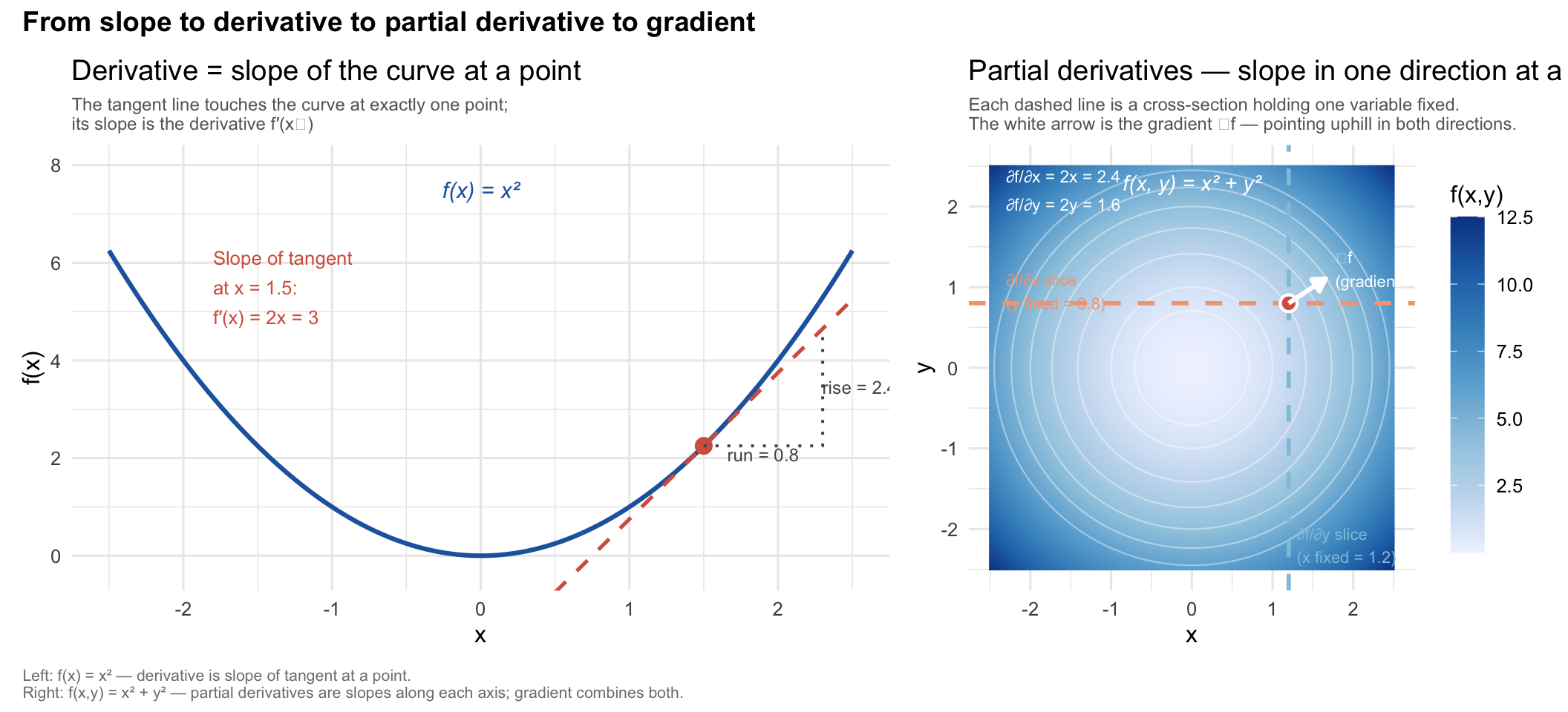
Three-sentence summary (illustrated in Figure 11.9):

A derivative is a slope at a point on a curve. A partial derivative is a slope in one direction when the function depends on many variables. A gradient is the full collection of all partial derivatives — a compass that points the network uphill so gradient descent can walk it downhill.

---

11.4.5.1 The Backpropagation Update Rule

The Update Rule is simply the formula used to update (adjust) the parameters (weights and biases) for any given node.

For any parameter \(\theta\) (a weight \(w_{kj}\) or bias \(w_{k0}\) or output weight \(\beta_k\)):

\[\theta^{\text{new}} = \theta^{\text{old}} - \eta \cdot \frac{\partial R}{\partial \theta} \tag{11.35}\]

where \(\eta\) (eta) is the learning rate, a small positive number for limiting how large each update step can be (shrinking the step size).

How is \(\frac{\partial R}{\partial \theta}\) calculated?

The total loss \(R(\theta) = \sum_{i=1}^{n} \text{Loss}_i\) is a composition of functions where

• the total loss depends on the prediction,
• which depends on the output weights,
• which depend on Layer 2 activations feeding the output layer,
• which depend on Layer 2 weights acting on the inputs from the previous layer, and
• so on back to the inputs.

The chain rule of calculus allows us to decompose (factor) this into a product of simpler derivatives, one factor per link (layer) in the chain.

11.4.5.2 Update Rule for the Output Layer

For a parameter \(\beta_k\) at the output layer there are only two factors in the chain in Equation 11.36.

• Since \(\beta_k\) sits at the very end of the network, directly connecting Layer 2 activations to the prediction, there are no intervening activation functions or additional layers between \(\beta_k\) and the loss:

\[\frac{\partial R_i}{\partial \beta_k} = \underbrace{\frac{\partial \text{Loss}_i}{\partial \hat{y}_i}}_{\text{(1) how sensitive is}\atop\text{the loss to the prediction?}} \cdot \underbrace{\frac{\partial \hat{y}_i}{\partial \beta_k}}_{\text{(2) how much does}\atop\beta_k\text{ move the prediction?}} \tag{11.36}\]

These two factors answer two distinct questions:

• Factor (1): the error signal: \(\dfrac{\partial \text{Loss}_i}{\partial \hat{y}_i}\) asks “in which direction, and by how much, does the loss change if the prediction \(\hat{y}_i\) nudges up by a tiny amount?“

  Differentiating squared-error loss (Equation 11.29) with respect to \(\hat{y}_i\) gives: \[\frac{\partial \text{Loss}_i}{\partial \hat{y}_i} = -(y_i - \hat{y}_i) \tag{11.37}\] This is the negative (of the) residual.

  • If the model under-predicted (\(\hat{y}_i < y_i\)), the residual is positive so the gradient is negative which means increasing \(\hat{y}_i\) reduces the loss.
  • If the model over-predicted, the gradient is positive, so increasing \(\hat{y}_i\) would make things worse.
  • The sign and magnitude of this factor tell the network how wrong it was and in which direction.

• Factor (2): the leverage of \(\beta_k\): \(\dfrac{\partial \hat{y}_i}{\partial \beta_k}\) asks “if \(\beta_k\) increases by a tiny amount, how much does the prediction \(\hat{y}_i\) change?”

• Since the prediction follows Equation 11.28, differentiating with respect to \(\beta_k\) gives: \[\frac{\partial \hat{y}_i}{\partial \beta_k} = A^{(2)}_k \tag{11.38}\]

• Each output parameter \(\beta_k\) multiplies its own activation \(A^{(2)}_k\) in the prediction formula so the activation is exactly how much that parameter moves the prediction.

  • A large \(A^{(2)}_k\) means \(\beta_k\) has high leverage; a zero activation (e.g. a dead ReLU node upstream) means \(\beta_k\) has no influence on the prediction for that observation, and its gradient will be zero so it receives no update.

Combining the two factors gives the full gradient:

\[\dfrac{\partial R_i}{\partial \beta_k} = \underbrace{-(y_i - \hat{y}_i)}_{\text{how wrong, and}\atop\text{in which direction}} \cdot \underbrace{A^{(2)}_k}_{\text{how much }\beta_k\text{ is}\atop\text{responsible for that error}} \tag{11.39}\]

This product is the core logic of learning: the update to \(\beta_k\) is large when the model made a big error and \(\beta_k\)’s node was highly active (i.e., \(A^{(2)}_k\) was large).

• If the node was inactive (\(A^{(2)}_k = 0\)), there is no gradient and no update since the parameter had no causal role in producing the error, so it should not be penalized.

11.4.5.3 Update Rule for the Last Hidden Layer

Once the output layer update rule is know, we moving back to the last hidden.

By moving backwards to a parameter \(w^{(2)}_{m,j}\) in Hidden Layer 2, the update rule structure changes in a critical way.

• In the output-layer gradient Equation 11.39, \(A^{(2)}_k\) appeared as Factor (2) since it was the final, fixed input to \(\beta_k\); it was a number we could simply read off.
• Now \(A^{(2)}_m\) is no longer fixed: it is itself a function of the node’s weights, \(w^{(2)}_{m,j}\), that calculated the pre-activation score \(z^{(2)}_{m,i}\).

So Factor (2) cannot simply be appended; it must be replaced and expanded:

• The derivative that was Factor (2) is still present structurally, but what it evaluates to has changed.

• In the output-layer case we asked: *“how does* \(\hat{y}_i\) change if \(\beta_k\) changes?” and the answer was \(A^{(2)}_k\).

  • The activation popped out because the variable \(\beta_k\) is directly multiplied by \(A^{(2)}_k\) in Equation 11.28.

• Now we are asking a different question: *“how does* \(\hat{y}_i\) change if \(A^{(2)}_m\) changes?” so we return to Equation 11.28:

  \[\hat{y}_i = \beta_0 + \beta_1 A^{(2)}_1 + \beta_2 A^{(2)}_2 + \cdots + \beta_{K_2} A^{(2)}_{K_2}\]

Now, differentiating with respect to \(A^{(2)}_m\) requires treating it as the variable so every term vanishes except the one that contains \(A^{(2)}_m\), leaving:

\[\frac{\partial \hat{y}_i}{\partial A^{(2)}_m} = \beta_m \tag{11.40}\]

The answer in Equation 11.40 is now \(\beta_m\), not \(A^{(2)}_m\).

• The roles of weight and activation have swapped:

  • differentiating \(\beta_m \cdot A^{(2)}_m\) with respect to the weight \(\beta_m\) gives \(A^{(2)}_m\);
  • differentiating the same product with respect to the activation \(A^{(2)}_m\) gives \(\beta_m\).

• This swap is the key algebraic shift when stepping back one layer: the same prediction formula, differentiated with respect to a different quantity, produces the other member of the weight–activation pair.

• Two new links are then added to continue the chain from \(A^{(2)}_m\) back to \(w^{(2)}_{m,j}\), because \(A^{(2)}_m\) is not a free variable, it was produced by applying \(g(\cdot)\) to \(z^{(2)}_{m,i}\), which in turn depended on \(w^{(2)}_{m,j}\):

  • Factor (3): how \(A^{(2)}_m\) responds to its own pre-activation \(z^{(2)}_{m,i}\), the activation gate \(g'(\cdot)\)
  • Factor (4): how \(z^{(2)}_{m,i}\) responds to the weight \(w^{(2)}_{m,j}\), this is \(A^{(1)}_{j,i}\), the Layer 1 activation that \(w^{(2)}_{m,j}\) scaled (the same leverage logic as Equation 11.38, now one layer back)

The resulting four-factor chain is (Equation 11.41):

\[\begin{aligned} \frac{\partial R_i}{\partial w^{(2)}_{m,j}} &= \underbrace{\frac{\partial \text{Loss}_i}{\partial \hat{y}_i}}_{\text{(1) loss gradient, unchanged}} \cdot \underbrace{\frac{\partial \hat{y}_i}{\partial A^{(2)}_m}}_{\text{(2) }A^{(2)}_m\text{'s influence on prediction} = \beta_m} \\[18pt] &\quad \cdot \underbrace{\frac{\partial A^{(2)}_m}{\partial z^{(2)}_{m,i}}}_{\text{(3) activation gate } g'(\cdot)\text{ replaces }A^{(2)}_k} \cdot \underbrace{\frac{\partial z^{(2)}_{m,i}}{\partial w^{(2)}_{m,j}}}_{\text{(4) weight's input} = A^{(1)}_{j,i}} \end{aligned} \tag{11.41}\]

Notice the conceptual parallel with the output-layer gradient (Table 11.15):

Table 11.15: Structural parallel between output-layer and Layer 2 chain rule gradients.

	Output layer (\(\partial R_i / \partial \beta_k\))	Layer 2 (\(\partial R_i / \partial w^{(2)}_{m,j}\))
Factor (1)	\(-(y_i - \hat{y}_i)\) — error signal	same, unchanged
Factor (2)	\(A^{(2)}_k\) — the activation is the leverage of \(\beta_k\)	\(\beta_m\) — now the leverage of \(A^{(2)}_m\) on the prediction; the activation has moved deeper
Factor (3)	(not needed — no activation between \(\beta_k\) and \(\hat{y}_i\))	\(g'(z^{(2)}_{m,i})\) — did \(A^{(2)}_m\)’s node fire?
Factor (4)	(not needed — \(\beta_k\) directly multiplies \(A^{(2)}_k\))	\(A^{(1)}_{j,i}\) — the input that \(w^{(2)}_{m,j}\) scaled

In short: every time we step one layer further back, the activation that was the endpoint (the leverage term) becomes an intermediate node that must itself be differentiated — adding two new links while the old leverage term transforms into the next layer’s output weight.

The factor descriptions:

• Factor (1): \(-(y_i - \hat{y}_i)\) : same error signal as before; it always originates at the output
• Factor (2): \(\dfrac{\partial \hat{y}_i}{\partial A^{(2)}_m} = \beta_m\) : the output-layer weight connecting \(A^{(2)}_m\) to the prediction; this is the “importance” of node \(m\)’s activation to the final output
• Factor (3): \(g'(z^{(2)}_{m,i})\) : the activation gate; determines whether the error signal passes back through node \(m\) (ReLU: 0 or 1; sigmoid: small positive value; linear: 1 always)
• Factor (4): \(\dfrac{\partial z^{(2)}_{m,i}}{\partial w^{(2)}_{m,j}} = A^{(1)}_{j,i}\) : the Layer 1 activation that fed into \(w^{(2)}_{m,j}\); the same “leverage” logic as before, now one layer back

Combining Equation 11.41:

\[\dfrac{\partial R_i}{\partial w^{(2)}_{m,j}} = -(y_i - \hat{y}_i) \cdot \beta_m \cdot g'(z^{(2)}_{m,i}) \cdot A^{(1)}_{j,i} \tag{11.42}\]

11.4.5.4 Moving back From One Hidden Layer to its Previous Hidden Layer

For a weight in Hidden Layer 1, the chain extends one further layer:

\[\frac{\partial R_i}{\partial w^{(1)}_{k,j}} = \underbrace{-(y_i - \hat{y}_i)}_{\text{(1) loss gradient}} \cdot \underbrace{\left(\sum_m \beta_m \cdot g'(z^{(2)}_{m,i}) \cdot w^{(2)}_{m,k}\right)}_{\text{(2)--(4) accumulated error from L2,}\atop\text{summed over all L2 nodes }m} \cdot \underbrace{g'(z^{(1)}_{k,i})}_{\text{(5) L1 activation}\atop\text{gate}} \cdot \underbrace{X_{j,i}}_{\text{(6) input}\atop\text{value}} \tag{11.43}\]

The summation \(\sum_m\) arises because Layer 1 node \(k\) sends its output to all Layer 2 nodes; the error flowing back from each of those paths must be collected together. This is the key structural difference from the output-layer calculation.

Intuition for each factor (Table 11.16):

Table 11.16: Intuition for each factor in the chain rule product.

Factor	Symbol	Answers the question…
Loss gradient	\(-(y_i - \hat{y}_i)\) or \(\hat{P}(m)-\mathbf{1}[y_i=m]\)	How wrong was the final prediction?
Output/layer weight	\(\beta_m\) or \(w^{(2)}_{m,k}\)	How much does this node’s output influence the error?
Activation gate \(g'(\cdot)\)	\(\mathbf{1}[z>0]\), \(g(z)(1-g(z))\), or \(1\)	Did this node “fire”? ReLU shuts gradient off completely when \(z \le 0\)
Input to the weight	\(A^{(l)}_{j,i}\) or \(X_{j,i}\)	What was the incoming signal that this weight scaled?

Warning 11.1: ⚠️ The Cascading Zero Problem: How ReLU Blocks Gradient Flow

The ReLU activation gate \(g'(z) = \mathbf{1}[z > 0]\) is either exactly 1 or exactly 0 — there is no in-between. This binary behavior has an important consequence: a zero at any point in the chain rule product zeroes out the entire gradient for that path, regardless of how large the other factors are.

The chain rule is a product. Recall the full gradient for a Layer 1 weight:

\[\frac{\partial R_i}{\partial w^{(1)}_{k,j}} = -(y_i - \hat{y}_i) \cdot \left(\sum_m \beta_m \cdot \underbrace{g'(z^{(2)}_{m,i})}_{\text{Layer 2 gate}} \cdot w^{(2)}_{m,k}\right) \cdot \underbrace{g'(z^{(1)}_{k,i})}_{\text{Layer 1 gate}} \cdot X_{j,i}\]

If any gate in this chain is zero, the product is zero and \(w^{(1)}_{k,j}\) receives no update at all that observation (Table 11.17):

Table 11.17: Effect of ReLU gate scenarios on gradient flow to Layer 1 weights.

Scenario	Effect on gradient for \(w^{(1)}_{k,j}\)
Layer 1 node \(k\) had \(z^{(1)}_{k,i} \le 0\)	\(g'(z^{(1)}_{k,i}) = 0\) → gradient is 0; \(w^{(1)}_{k,j}\) not updated regardless of what happens downstream
Layer 2 node \(m\) had \(z^{(2)}_{m,i} \le 0\)	\(g'(z^{(2)}_{m,i}) = 0\) → that particular path through \(m\) contributes 0 to the \(\sum_m\) term; other Layer 2 nodes may still carry a gradient
All Layer 2 nodes had \(z^{(2)}_{m,i} \le 0\)	Every term in \(\sum_m\) is 0 → the entire bracketed sum is 0 → \(w^{(1)}_{k,j}\) still not updated, even if Layer 1 node \(k\) itself was active

Layer 2 zeroes “shadow” Layer 1. Even if Layer 1 node \(k\) fired (\(z^{(1)}_{k,i} > 0\), so its own gate is open), if every Layer 2 node that receives from \(k\) was itself dead (\(z^{(2)}_{m,i} \le 0\) for all \(m\)), then no error signal reaches the Layer 1 weights. The gradient is zeroed out before it arrives.

This is called the dying ReLU problem. A node that outputs 0 for every observation in the batch stops receiving any gradient signal; its weights are frozen and it can never recover during that training run.

Why does it still happen in practice? Two reasons:

1. Not all observations zero out the same nodes — across a batch of 10 observations, a node may be dead for some \(i\) and alive for others; the weight update averages over all \(i\), so partial signal still gets through as long as the node fires for at least one observation.
2. Biases: a large negative bias \(w_{k,0}\) can push \(z_{k,i}\) below 0 for all observations, permanently killing the node.

Comparison across activation functions (Table 11.18):

Table 11.18: Gradient behavior comparison across activation functions.

Activation	\(g'(z)\)	Gradient blocked when…	Can recover?
ReLU	\(\mathbf{1}[z > 0]\)	\(z \le 0\) — hard zero	No (for that obs / epoch)
Sigmoid	\(g(z)(1-g(z))\)	\(z \ll 0\) or \(z \gg 0\) (saturation)	Slowly — gradient very small but non-zero
Linear	\(1\) always	Never	N/A — always passes full gradient

This is one practical reason why weight initialization matters: Xavier/Glorot initialization (Step 1) is designed to keep pre-activations \(z\) near zero at the start of training, where ReLU is active and gradients flow freely.

---

11.4.5.5 Step-by-Step Case A: Regression Case (Movie Attendance)

11.4.5.5.1 The Output Layer for Regression

The residual for observation \(i\) is the prediction error:

\[\delta^{\text{out}}_i = -(y_i - \hat{y}_i) = -(6.1 - 5.52) = -0.58\]

The gradient for each output parameter \(\beta_k\) follows Equation 11.39:

\[\frac{\partial R_i}{\partial \beta_k} = -(y_i - \hat{y}_i) \cdot A^{(2)}_k = -0.58 \cdot A^{(2)}_k\]

For \(k=1\): \(\frac{\partial R_i}{\partial \beta_1} = (-0.58)(0.075) = -0.0435\)

For \(k=2\): \(\frac{\partial R_i}{\partial \beta_2} = (-0.58)(1.230) = -0.7134\)

With learning rate \(\eta = 0.01\), applying the update rule (Equation 11.35):

\[\beta_1^{\text{new}} = 2.80 - (0.01)(-0.0435) = 2.80 + 0.000435 \approx \mathbf{2.8004}\]

\[\beta_2^{\text{new}} = 3.10 - (0.01)(-0.7134) = 3.10 + 0.007134 \approx \mathbf{3.107}\]

Both output weights increased slightly as the model is adjusting to predict a higher attendance (moving toward the true value of 6.1).

11.4.5.5.2 Propagating to Hidden Layer 2 for Regression

The error signal is passed backward to Layer 2.

For each parameter \(w^{(2)}_{m,j}\) in Layer 2, using Equation 11.42:

\[\frac{\partial R_i}{\partial w^{(2)}_{m,j}} = -(y_i - \hat{y}_i) \cdot \beta_m \cdot g'\!\left(z^{(2)}_{m,i}\right) \cdot A^{(1)}_{j,i}\]

where \(g'(z)\) is the derivative of the activation function:

• ReLU: \(g'(z) = 1\) if \(z > 0\), else \(0\)
• Sigmoid: \(g'(z) = g(z)(1 - g(z))\)
• Linear: \(g'(z) = 1\)

For Layer 2, node \(m=1\) (where \(z^{(2)}_{1,1} = 0.075 > 0\), so \(g'=1\) under ReLU), and Layer 1 output \(A^{(1)}_{1} = 0.972\):

\[\frac{\partial R_i}{\partial w^{(2)}_{1,1}} = (-0.58)(2.80)(1)(0.972) = \mathbf{-1.578}\]

\[w^{(2),\text{new}}_{1,1} = -0.30 - (0.01)(-1.578) = -0.30 + 0.016 = \mathbf{-0.284}\]

---

11.4.5.5.3 Propagating to Hidden Layer 1 for Regression

The error continues to travel backward. For parameter \(w^{(1)}_{k,j}\) in Layer 1, using Equation 11.43:

\[\frac{\partial R_i}{\partial w^{(1)}_{k,j}} = -(y_i - \hat{y}_i) \cdot \left(\sum_{m} \beta_m \cdot g'\!\left(z^{(2)}_{m,i}\right) \cdot w^{(2)}_{m,k}\right) \cdot g'\!\left(z^{(1)}_{k,i}\right) \cdot X_{j,i}\]

This is the full chain rule (Equation 11.43): output error → Layer 2 weights → Layer 2 activation → Layer 1 weights → Layer 1 activation → input.

---

11.4.5.6 Step-by-Step Case B: Classification (Movie Hit/Flop)

11.4.5.6.1 The Output Layer for Classification

For cross-entropy loss (Equation 11.33) with softmax (Equation 11.9), the gradient at the output layer has a remarkably clean form. The error signal for class \(m\) for observation \(i\) is:

\[\delta^{\text{out}}_{i,m} = \hat{P}(m | x_i) - \mathbf{1}[y_i = m] \tag{11.44}\]

That is, predicted probability minus the indicator of whether \(m\) was the true class.

For our example where \(y_1 = \text{Hit}\) (\(m=2\)):

\[\delta^{\text{out}}_{i,1} = 0.037 - 0 = \mathbf{+0.037} \quad \text{(Flop: over-predicted slightly)}\]

\[\delta^{\text{out}}_{i,2} = 0.963 - 1 = \mathbf{-0.037} \quad \text{(Hit: under-predicted slightly)}\]

These small errors confirm the model is already close; the weight updates will be minor. For a wrong, confident prediction these errors would be large, driving larger updates.

11.4.5.6.2 The Hiddem Layers for Classification

The gradients propagate backward through both hidden layers exactly as in the regression case, using the chain rule layer by layer.

11.4.5.7 After Completing the Backwards Pass for All 10 Observations, One Epoch is Complete

After computing the forward pass, the gradients, and the backwards pass (backpropagation) to update all the weights and biases in all layers and nodes for all \(n = 10\) observations, the first epoch is complete.

In practice however, each set of calculations for the forward pass, the output layer, and the backwards updating of the weights and biases are computed across all 10 observations simultaneously using matrix algebra.

11.4.6 Using Matrix Algebra to Execute an Epoch

Updating one weight at a time in a loop would be mathematically correct but computationally prohibitive!

• A network with even a few hundred nodes has thousands of parameters, and doing so for thousands of epochs over millions of observations is impractical.
• Instead, all gradients are computed and all parameters updated simultaneously pass using matrix algebra, which modern hardware (GPUs) executes in parallel.

The key insight is the forward and backward passes across all \(n\) observations can be written as matrix operations.

• Rather than computing \(z_{k,i}\) one observation at a time, as in Equation 11.23, we stack all the observations into matrices and process them simultaneously.

11.4.6.1 Stacking Observations and Parameters into Matrices

We start with two matrices

• Stack all input observations into a matrix \(\mathbf{X}\), and,
• Stack all the Layer 1 weights and biases into a matrix \(\mathbf{W}^{(1)}\):

\[\mathbf{X} = \begin{bmatrix} 1 & X_{1,1} & \cdots & X_{p,1} \\ 1 & X_{1,2} & \cdots & X_{p,2} \\ \vdots & \vdots & \ddots & \vdots \\ 1 & X_{1,n} & \cdots & X_{p,n} \end{bmatrix}_{n \times (p+1)} \qquad \mathbf{W}^{(1)} = \begin{bmatrix} w_{1,0} & w_{2,0} & \cdots & w_{K_1,0} \\ w_{1,1} & w_{2,1} & \cdots & w_{K_1,1} \\ \vdots & \vdots & \ddots & \vdots \\ w_{1,p} & w_{2,p} & \cdots & w_{K_1,p} \end{bmatrix}_{(p+1) \times K_1} \tag{11.45}\]

• The leading column of 1s in \(\mathbf{X}\) captures the bias terms \(w_{k,0}\), so biases require no separate bookkeeping.

11.4.6.2 A Forward Pass with Matrices

The entire Layer 1 pre-activation calculation, for all nodes and all observations at once, is then a single matrix multiplication to create a matrix \(\mathbf{Z}^{(1)}\):

\[\mathbf{Z}^{(1)} = \mathbf{X} \mathbf{W}^{(1)}, \qquad \mathbf{Z}^{(1)} \in \mathbb{R}^{n \times K_1} \tag{11.46}\]

• Entry \((i, k)\) of \(\mathbf{Z}^{(1)}\) is exactly \(z_{k,i}\) from Equation 11.23, the pre-activation for node \(k\), observation \(i\).
• All \(n \times K_1\) values are produced by one operation.

Applying the activation function element-wise to every entry:

\[\mathbf{A}^{(1)} = g\!\left(\mathbf{Z}^{(1)}\right), \qquad \mathbf{A}^{(1)} \in \mathbb{R}^{n \times K_1} \tag{11.47}\]

Layer 2 follows the identical pattern (pre-pending a bias column of 1s to \(\mathbf{A}^{(1)}\), denoted \(\tilde{\mathbf{A}}^{(1)}\)):

\[\mathbf{Z}^{(2)} = \tilde{\mathbf{A}}^{(1)} \mathbf{W}^{(2)}, \qquad \mathbf{A}^{(2)} = g\!\left(\mathbf{Z}^{(2)}\right) \tag{11.48}\]

11.4.6.3 Stacking Gradients for the Simultaneous Update

The gradient of the total loss with respect to the output weight vector is the sum of per-observation gradients from Equation 11.39.

Stacked over all \(n\) observations, this becomes:

\[\frac{\partial R}{\partial \mathbf{W}^{\text{out}}} = \left(\mathbf{A}^{(2)}\right)^\top \boldsymbol{\delta}^{\text{out}}, \qquad \boldsymbol{\delta}^{\text{out}} = -({\mathbf{y} - \hat{\mathbf{y}}}) \in \mathbb{R}^{n \times 1} \tag{11.49}\]

• The matrix product \((\mathbf{A}^{(2)})^\top \boldsymbol{\delta}^{\text{out}}\) accumulates every observation’s contribution in one step; the matrix form of \(\sum_i \frac{\partial R_i}{\partial \beta_k}\).

11.4.6.4 Usng a Matrix to Update (Backpropagate) Hidden Layer 2

This is the matrix form of Equation 11.41:

\[\boldsymbol{\Delta}^{(2)} = \boldsymbol{\delta}^{\text{out}} \left(\mathbf{W}^{\text{out}}\right)^\top \odot g'\!\left(\mathbf{Z}^{(2)}\right), \qquad \frac{\partial R}{\partial \mathbf{W}^{(2)}} = \left(\tilde{\mathbf{A}}^{(1)}\right)^\top \boldsymbol{\Delta}^{(2)} \tag{11.50}\]

• The \(\odot\) symbol denotes element-wise multiplication (the Hadamard product)
• This is where the activation gate \(g'(\cdot)\) is applied to every entry of \(\mathbf{Z}^{(2)}\) simultaneously.
• Any row where all entries of \(g'(\mathbf{Z}^{(2)})\) are zero (dead ReLU nodes for that observation) zeroes out the entire corresponding row of \(\boldsymbol{\Delta}^{(2)}\), blocking gradient flow for that observation; the matrix manifestation of the cascading-zero effect discussed in Equation 11.43.

11.4.6.5 Using a Matrix to Update (Backpropagate) Hidden Layer 2

This is the matrix form of Equation 11.43:

\[\boldsymbol{\Delta}^{(1)} = \boldsymbol{\Delta}^{(2)} \left(\mathbf{W}^{(2)}\right)^\top \odot g'\!\left(\mathbf{Z}^{(1)}\right), \qquad \frac{\partial R}{\partial \mathbf{W}^{(1)}} = \mathbf{X}^\top \boldsymbol{\Delta}^{(1)} \tag{11.51}\]

• The matrix product \(\boldsymbol{\Delta}^{(2)}(\mathbf{W}^{(2)})^\top\) is precisely the \(\sum_m\) over all Layer 2 nodes in Equation 11.43.
• Every path from Layer 1 through all Layer 2 nodes is accumulated in one operation.

11.4.6.6 The Simultaneous Update Step

With all gradient matrices computed from the current (pre-update) weights, the update rule Equation 11.35 is applied to all parameters at once:

\[\mathbf{W}^{(1)} \leftarrow \mathbf{W}^{(1)} - \eta \cdot \frac{\partial R}{\partial \mathbf{W}^{(1)}} \tag{11.52}\]

\[\mathbf{W}^{(2)} \leftarrow \mathbf{W}^{(2)} - \eta \cdot \frac{\partial R}{\partial \mathbf{W}^{(2)}}\]

\[\mathbf{W}^{\text{out}} \leftarrow \mathbf{W}^{\text{out}} - \eta \cdot \frac{\partial R}{\partial \mathbf{W}^{\text{out}}}\]

All three updates use gradients computed from the weights before any update occurred.

• This is what makes the update truly simultaneous: no layer sees partially-updated parameters from another layer during the backward pass.

11.4.6.7 Matrix Algebra Summary for One Epoch

Our example (\(n=10\), \(p=5\), \(K_1=4\), \(K_2=3\))

Table 11.19: Matrix operations and dimensions for one forward–backward pass (\(n=10\), \(p=5\), \(K_1=4\), \(K_2=3\)).

Operation	Matrix form	Dimensions
Forward: L1 pre-activation	\(\mathbf{Z}^{(1)} = \mathbf{X}\mathbf{W}^{(1)}\)	\((10 \times 6)(6 \times 4) \to 10 \times 4\)
Forward: L1 activation	\(\mathbf{A}^{(1)} = g(\mathbf{Z}^{(1)})\)	\(10 \times 4\)
Forward: L2 pre-activation	\(\mathbf{Z}^{(2)} = \tilde{\mathbf{A}}^{(1)}\mathbf{W}^{(2)}\)	\((10 \times 5)(5 \times 3) \to 10 \times 3\)
Forward: L2 activation	\(\mathbf{A}^{(2)} = g(\mathbf{Z}^{(2)})\)	\(10 \times 3\)
Forward: prediction	\(\hat{\mathbf{y}} = \tilde{\mathbf{A}}^{(2)}\boldsymbol{\beta}\)	\((10 \times 4)(4 \times 1) \to 10 \times 1\)
Output error	\(\boldsymbol{\delta}^{\text{out}} = -(\mathbf{y} - \hat{\mathbf{y}})\)	\(10 \times 1\)
Backward: output gradient	\((\mathbf{A}^{(2)})^\top \boldsymbol{\delta}^{\text{out}}\)	\((3 \times 10)(10 \times 1) \to 3 \times 1\)
Backward: L2 delta	\(\boldsymbol{\delta}^{\text{out}}(\boldsymbol{\beta})^\top \odot g'(\mathbf{Z}^{(2)})\)	\(10 \times 3\)
Backward: L2 gradient	\((\tilde{\mathbf{A}}^{(1)})^\top \boldsymbol{\Delta}^{(2)}\)	\((5 \times 10)(10 \times 3) \to 5 \times 3\)
Backward: L1 delta	\(\boldsymbol{\Delta}^{(2)}(\mathbf{W}^{(2)})^\top \odot g'(\mathbf{Z}^{(1)})\)	\(10 \times 4\)
Backward: L1 gradient	\(\mathbf{X}^\top \boldsymbol{\Delta}^{(1)}\)	\((6 \times 10)(10 \times 4) \to 6 \times 4\)

• Note how the \(\odot\) rows are where ReLU’s dead-node effect appears in matrix form: a zero in \(g'(\mathbf{Z}^{(l)})\) zeroes the corresponding entry of \(\boldsymbol{\Delta}^{(l)}\), cutting off gradient flow for that node and observation.

The process repeats for each epoch:

1. Forward pass: compute \(\mathbf{Z}^{(1)}, \mathbf{A}^{(1)}, \mathbf{Z}^{(2)}, \mathbf{A}^{(2)}, \hat{\mathbf{y}}\) (or \(\hat{\mathbf{P}}\)) via Equation 11.46–Equation 11.48
2. Compute loss: MSE (Equation 11.30) or cross-entropy (Equation 11.34) over all \(n\) observations
3. Backward pass: compute \(\boldsymbol{\delta}^{\text{out}}, \boldsymbol{\Delta}^{(2)}, \boldsymbol{\Delta}^{(1)}\) via Equation 11.50–Equation 11.51
4. Update all parameters simultaneously: apply Equation 11.52 to all weight matrices at once using the frozen gradient matrices

Over many epochs, the weight matrices converge to values that minimize the loss on the training data and, ideally, generalize well to new data.

Note 11.1: 🎮 Why GPUs? From Video Games to Neural Networks

The matrix multiplications in Table 11.19, Equation 11.46 through Equation 11.51, are computationally cheap for our 10-observation example.

• At real-world scale, with billions of parameters, they are among the most demanding computations humans have ever designed.
• Understanding why GPUs handle them efficiently requires a short detour into the history of video games.

11.4.6.7.0.1 The unexpected origin: video game rendering

A video game must render a three-dimensional virtual world onto a flat screen 60 or more times per second. - Every surface in that world is represented as a mesh of triangles. - Moving each triangle from 3-D world-space to 2-D screen-space requires multiplying its \((x, y, z)\) coordinates by a series of transformation matrices (rotation, scaling, perspective projection). - A single frame of a modern game may involve tens of millions of these matrix operations, all of which must finish within ~16 milliseconds.

Chip designers in the 1990s–2000s (NVIDIA, ATI/AMD) solved this by building special processors with thousands of small, simple arithmetic cores that execute matrix multiplications in parallel: the Graphics Processing Unit (GPU).

• A CPU has 8–64 large, general-purpose cores optimized for sequential logic; a GPU has 3,000–16,000 small cores optimized for doing the same arithmetic operation on thousands of numbers simultaneously.

When researchers in the early 2010s (most famously AlexNet, 2012) began training neural networks on GPUs, they discovered that the forward and backward passes (Equation 11.46–Equation 11.51) are structurally identical to the matrix operations in game rendering: large matrix multiplications that are embarrassingly parallel.

• Training time that took weeks on CPUs dropped to days or hours on GPUs.
• The deep learning revolution that followed was in large part a consequence of commodity gaming hardware.

11.4.6.7.0.2 Model scale in 2025

The table below places Table 11.19 in context.

• Every model below is structurally identical to our worked example; the same forward pass, the same chain rule, the same update rule (Equation 11.35), just with more layers, more nodes, and far more parameters.

Table 11.20: Parameter counts and compute requirements for neural network models of varying scale.

Scale	Example models	Parameters	Training hardware	Training time
Toy	This worked example	61	Spreadsheet / CPU	Milliseconds
Small	LeNet, shallow MLP	100K–1M	Laptop CPU	Minutes
Medium	ResNet-50, BERT-base	25M–110M	1–4 GPUs	Hours–days
Large	GPT-2, ViT-L	1.5B–300M	8–64 GPUs	Days–weeks
Frontier	GPT-4 (~1.8T est.), Llama 3 405B	100B–2T	1,000s of GPUs	Months

A single training step of GPT-3 (175 billion parameters) requires approximately \(3.14 \times 10^{23}\) floating-point operations (Brown et al. 2020).

• At 125 TFLOPS (fp16) per NVIDIA A100 GPU, that would take one GPU roughly \(8 \times 10^7\) seconds or about 2.5 years.
• OpenAI trained it on ~10,000 GPUs in parallel over several months.

11.4.7 What this means for this course

The architecture in this worked example scales directly to frontier models.

• GPT-4 is, at its core, a very deep network of matrix multiplications and non-linear activations, the same operations in Table 11.19, repeated \(\sim 10^{11}\) times per forward pass instead of the 11 operations shown there.

The practical implication: for problems in this course, a laptop CPU or a free Google Colab GPU is sufficient.

• For problems at industry or research scale, compute cost is a primary design constraint, one reason why transfer learning (Section 11.14) and fine-tuning are so important: they let you build on a frontier model’s pre-learned weights rather than incurring the cost of training from scratch.

---

11.4.8 Summary: Regression vs. Classification

Table 11.21 collects the key differences between the regression and classification cases across every stage covered in this worked example.

Table 11.21: Side-by-side summary of regression vs. classification across all stages.

Stage	Regression (Attendance)	Classification (Hit?)
Input	5 features per observation	Same 5 features
Hidden Layer 1	\(z = w_0 + \sum w_j X_j\); apply ReLU	Same
Hidden Layer 2	\(z^{(2)} = w^{(2)}_0 + \sum w^{(2)}_m A^{(1)}_m\); apply ReLU	Same
Output activation	Linear (\(\hat{y} = \beta_0 + \sum \beta_k A^{(2)}_k\))	Softmax (\(\hat{P}(m) = e^{Z_m}/\sum e^{Z_l}\))
Loss function	MSE \(\frac{1}{2}(y - \hat{y})^2\)	Cross-Entropy \(-\log \hat{P}(y)\)
Output layer gradient	\(-(y_i - \hat{y}_i)\)	\(\hat{P}(m) - \mathbf{1}[y_i=m]\)
Interpretation	Predicted continuous value	Predicted class probabilities (sum to 1)

---

11.4.9 Practice Exercise: Observation \(i = 2\)

The worked example traced observation \(i = 1\) through the full forward and backward pass.

Below are the values for observation \(i = 2\) so you can practice the same calculations yourself before checking the answers.

Given for observation \(i = 2\):

Quantity	Value
Inputs	\(X_1 = 0.9,\; X_2 = 1.4,\; X_3 = -0.6,\; X_4 = 0.3,\; X_5 = 1.1\)
True attendance (regression)	\(y_2 = 4.3\) million viewers
True class (classification)	\(y_2 = \text{Flop}\) (class 1)

Use the same initialized weights and biases from Step 1 (the network parameters have not yet been updated since we are still on the first forward pass before any gradient descent step).

🖊 Questions

Part A: Output layer (regression)

Using the Layer 2 activations you have already computed for \(i=2\) below:

\[A^{(2)}_{1,2} = 0.000, \quad A^{(2)}_{2,2} = 1.113, \quad A^{(2)}_{3,2} = 0.000\]

1. Compute the prediction \(\hat{y}_2\) using Equation 11.28 and the output weights \(\beta_0 = 1.50,\; \beta_1 = 2.80,\; \beta_2 = 3.10,\; \beta_3 = 0.95\).

2. Compute the per-observation squared-error loss \(\text{Loss}_2\) using Equation 11.29.

3. Compute the output-layer gradient \(\dfrac{\partial R_2}{\partial \beta_2}\) using Equation 11.39. Interpret the sign; should \(\beta_2\) increase or decrease on the next update?

Part B: Hidden Layer 2 gradient

4. Using the result from Part A and Layer 2 node \(m=2\) (which was active, \(z^{(2)}_{2,2} = 0.934 > 0\), so \(g'(z^{(2)}_{2,2}) = 1\) under ReLU), and the output weight \(\beta_2 = 3.10\), and the Layer 1 activation \(A^{(1)}_{1,2} = 0.972\) that fed into \(w^{(2)}_{2,1}\):

   Compute \(\dfrac{\partial R_2}{\partial w^{(2)}_{2,1}}\) using Equation 11.42. This is the gradient for the weight connecting Layer 1 node 1 to Layer 2 node 2 for observation 2.

5. Write out the update for \(w^{(2)}_{2,1}\) using Equation 11.35 with \(\eta = 0.01\). The current value is \(w^{(2)}_{2,1} = -0.30\).

Part C: Reflect

6. Layer 2 nodes 1 and 3 had \(A^{(2)}_{1,2} = 0\) and \(A^{(2)}_{3,2} = 0\) for this observation. What does that imply for the gradients \(\dfrac{\partial R_2}{\partial \beta_1}\) and \(\dfrac{\partial R_2}{\partial \beta_3}\)? Which section of the walkthrough explains why? (Hint: Warning 11.1.)

✅ Answers

Part A: Output layer (regression)

A1. Prediction \(\hat{y}_2\) (using Equation 11.28):

\[\hat{y}_2 = \beta_0 + \beta_1 A^{(2)}_{1,2} + \beta_2 A^{(2)}_{2,2} + \beta_3 A^{(2)}_{3,2}\]

\[= 1.50 + (2.80)(0.000) + (3.10)(1.113) + (0.95)(0.000)\]

\[= 1.50 + 0 + 3.450 + 0 = \mathbf{4.95 \text{ million viewers}}\]

A2. Squared-error loss (using Equation 11.29):

\[\text{Loss}_2 = \tfrac{1}{2}(y_2 - \hat{y}_2)^2 = \tfrac{1}{2}(4.3 - 4.95)^2 = \tfrac{1}{2}(0.65)^2 = \mathbf{0.211}\]

Compare to \(\text{Loss}_1 = 0.168\) from the main example, observation 2 has a slightly larger error.

A3. Output gradient \(\dfrac{\partial R_2}{\partial \beta_2}\) (using Equation 11.39):

\[\frac{\partial R_2}{\partial \beta_2} = -(y_2 - \hat{y}_2) \cdot A^{(2)}_{2,2} = -(4.3 - 4.95) \cdot 1.113 = -(-0.65)(1.113) = \mathbf{+0.723}\]

• The gradient is positive — the loss increases if \(\beta_2\) increases.
• The update rule (Equation 11.35) subtracts \(\eta\) times the gradient, so \(\beta_2\) will decrease slightly on the next step, pulling the prediction down toward the true value of 4.3.

Part B: Hidden Layer 2 gradient

B4. \(\dfrac{\partial R_2}{\partial w^{(2)}_{2,1}}\) (using Equation 11.42):

\[\frac{\partial R_2}{\partial w^{(2)}_{2,1}} = \underbrace{-(y_2 - \hat{y}_2)}_{-(-0.65)\,=\,+0.65} \cdot \underbrace{\beta_2}_{3.10} \cdot \underbrace{g'(z^{(2)}_{2,2})}_{1 \text{ (ReLU, active)}} \cdot \underbrace{A^{(1)}_{1,2}}_{0.972}\]

\[= 0.65 \times 3.10 \times 1 \times 0.972 = \mathbf{+1.959}\]

This is a fairly large gradient since Layer 1 node 1 was strongly active (\(A^{(1)}_{1,2} = 0.972\)) and is connected to an output-relevant Layer 2 node, so the error signal flows back strongly through this weight.

B5. Parameter update for \(w^{(2)}_{2,1}\) (using Equation 11.52):

\[w^{(2), \text{new}}_{2,1} = w^{(2), \text{old}}_{2,1} - \eta \cdot \frac{\partial R_2}{\partial w^{(2)}_{2,1}}\]

\[= -0.30 - (0.01)(1.959) = -0.30 - 0.0196 = \mathbf{-0.3196}\]

The weight becomes more negative; the network is reducing the influence of this connection because it contributed to an over-prediction.

# Given values
beta  <- c(1.50, 2.80, 3.10, 0.95)          # beta_0, beta_1, beta_2, beta_3
A2    <- c(0.000, 1.113, 0.000)              # Layer 2 activations obs 2
y2    <- 4.3                                  # true attendance
eta   <- 0.01                                 # learning rate

# A1: prediction
y_hat2 <- beta[1] + sum(beta[2:4] * A2)
cat("A1 prediction:", round(y_hat2, 3), "\n")

A1 prediction: 4.95 

# A2: loss
loss2 <- 0.5 * (y2 - y_hat2)^2
cat("A2 loss:", round(loss2, 3), "\n")

A2 loss: 0.211 

# A3: gradient for beta_2
grad_beta2 <- -(y2 - y_hat2) * A2[2]
cat("A3 gradient d_R/d_beta2:", round(grad_beta2, 3), "\n")

A3 gradient d_R/d_beta2: 0.724 

cat("   beta_2 update direction: ", ifelse(grad_beta2 > 0, "decrease", "increase"), "\n")

   beta_2 update direction:  decrease 

# B4: gradient for w^(2)_{2,1}
g_prime_z2  <- 1          # ReLU active
A1_node1    <- 0.972      # Layer 1 node 1 activation for obs 2
w_out_node2 <- 3.10       # beta_2
grad_w21    <- -(y2 - y_hat2) * w_out_node2 * g_prime_z2 * A1_node1
cat("B4 gradient d_R/d_w21:", round(grad_w21, 3), "\n")

B4 gradient d_R/d_w21: 1.959 

# B5: update
w21_old <- -0.30
w21_new <- w21_old - eta * grad_w21
cat("B5 w21 updated:", round(w21_new, 4), "\n")

B5 w21 updated: -0.3196 

Part C — Reflect

C6. When \(A^{(2)}_{1,2} = 0\) and \(A^{(2)}_{3,2} = 0\) (dead ReLU nodes for this observation):

\[\frac{\partial R_2}{\partial \beta_1} = -(y_2 - \hat{y}_2) \cdot A^{(2)}_{1,2} = (-0.65)(0) = \mathbf{0}\]

\[\frac{\partial R_2}{\partial \beta_3} = -(y_2 - \hat{y}_2) \cdot A^{(2)}_{3,2} = (-0.65)(0) = \mathbf{0}\]

Both output weights \(\beta_1\) and \(\beta_3\) receive zero gradient for observation 2; their nodes contributed nothing to the prediction, so they bear no responsibility for the error and are not updated.

• This is Factor (2) from Equation 11.39: the gradient is proportional to the activation, so a zero activation means no update.
• The deeper consequence, that dead Layer 2 nodes also block gradient flow back to Layer 1 weights, is explained in the cascading-zero callout.
• Even if a Layer 1 node fired, if every Layer 2 node it feeds into was dead for this observation, the Layer 1 weights receive no signal at all.

11.5 Training Options and Stopping

11.5.1 Batch, Mini-Batch, and Stochastic Gradient Descent

With so many calculations to be made, there are different approaches to how to use the training data in each epoch.

• Massive data sets can require many computations and significant memory to hold all the data at once.
• Research continues into multiple options for improving the speed and reducing the memory requirements for neural networks.

Each approach has trade offs between how long it takes to complete an epoch, how fast or slow to get to convergence, how smoothly to get to convergence, how to reduce bias or multicollinearity, and how much memory is required.

There are three popular approaches for how much data to include in each forward/backward pass through the network. See Batch, Mini Batch & Stochastic Gradient Descent.

• Batch Gradient Descent
  • All the observations are used at once, in a single batch or iteration.
  • When data space is “well-behaved”, it can provide for a smooth convergence across multiple epochs.
  • It does require all the data fit into memory at once.
• Stochastic Gradient Descent is the other extreme where only one observation at a time is fed into the model.
  • Thus there are \(n\) batches and each batch is processed in an iteration.
  • Much less data has to be computed each time and much less has to fit into memory.
  • The convergence can be less smooth as observations can vary widely.
• Mini-Batch Gradient Descent
  • This is in between the others where a fraction of the data is used for each batch.
  • If there are \(m\) batches, each batch uses \(n/m\) observations with the last batch using whatever remains after the \(m-1\)^st batch.
  • There are different methods for whether to update the \(\delta\)s after each mini-batch (do a backwards pass) or just store the residuals from a forward pass to update \(\delta\)s after all mini-batches have been run and you have \(n\) residuals.
  • There is some evidence that small batches (32) may be less smooth but converge more quickly and be more robust in prediction.
• Hybrid Approaches
  • One such method is to select the observations for each iteration at random (with/without replacement).
  • This would mean that perhaps not all \(n\) observations made it into each epoch.
  • Another method is to randomly shuffle all the input data at each epoch so different data goes into different batches for each epoch.

Note

Some use the term Stochastic Gradient Descent (SGD) as shorthand to refer to all the above approaches for selecting the data to be used in an iteration.

11.5.2 Optimization Algorithms

The discussion above covers how much data to use per update step.

• A separate question is how to move in the direction of the gradient, the choice of optimization algorithm (optimizer).
• ISLR2 uses standard gradient descent; in practice, almost all modern neural network training uses an adaptive optimizer that adjusts the effective learning rate per parameter automatically.

The core update rule (Equation 11.35 from the worked example) is:

\[\theta^{\text{new}} = \theta^{\text{old}} - \eta \cdot \frac{\partial R}{\partial \theta}\]

Adaptive optimizers modify this by maintaining running estimates of past gradients, allowing parameters that receive small or infrequent gradients to take larger steps and parameters with large consistent gradients to take smaller steps.

Table 11.22 lists the main choices:

Table 11.22: Common optimization algorithms for neural network training.

Optimizer	Key idea	When to prefer
SGD	Fixed \(\eta\), pure gradient step	Theoretical work; convex problems; CNNs with careful tuning
SGD + Momentum	Accumulates a velocity vector across steps; smooths oscillations	Image classification with CNNs
RMSProp	Divides \(\eta\) by a running average of squared gradients; adapts per parameter	Recurrent networks; was Keras default historically
Adam	Combines momentum (first moment) + RMSProp (second moment); bias-corrected	Default for most tasks — tabular, NLP, vision
AdamW	Adam with decoupled weight decay (L2 penalty applied separately from gradient)	Fine-tuning pre-trained transformer models

Adam (Kingma and Ba 2017) is the practical default for almost all deep learning work in 2025 and is the optimizer used in the examples below

• optimizer_rmsprop() is the Keras historical default but Adam is now preferred for new projects.
• The learning rate \(\eta\) (Table 11.29) still requires tuning as Adam’s adaptivity reduces sensitivity to the initial choice but does not eliminate it.

NoteAdam’s Key Ideas

• Momentum (first moment): Momentum keeps a running average of past gradients so it “remembers” which direction the parameters have been moving and keeps pushing that way, smoothing out noisy updates.
  • In statistics, the mean of a distribution is called the first moment, so this running average of gradients is the “first moment estimate.”
• RMSProp (second moment): RMSProp keeps a running average of past squared gradients. This measures how large the gradients have been recently, and uses it to scale the learning rate down for parameters that get large gradients and up for parameters that get small ones.
  • The mean of squared values is the second moment, hence “second moment estimate.”
• Bias-corrected: Early in training, both running averages start at zero, which biases them toward zero before they’ve had enough updates to reflect the true gradient history.
  • Adam applies a correction factor that compensates for this initialization bias, making the early updates more reliable.

11.5.3 When to Stop Training

Training is an iterative loop.

• After every epoch the parameters improve, but running too many epochs leads to overfitting where the model “memorizes” the training data and performs poorly on new observations.
• Two families of stopping criteria control this.

11.5.3.1 Loss-Based Convergence Threshold

The simplest approach monitors how much the training loss \(R\) changes from one epoch to the next:

\[\Delta R^{(t)} = R^{(t-1)} - R^{(t)} \tag{11.53}\]

Training stops when \(\Delta R^{(t)}\) falls below a pre-specified threshold \(\epsilon\) for \(p\) consecutive epochs:

\[\left| \Delta R^{(t)} \right| < \epsilon \quad \text{for } p \text{ consecutive epochs} \tag{11.54}\]

Both \(\epsilon\) and \(p\) are hyperparameters set before training begins (see Table 11.23):

Table 11.23: Stopping hyperparameters and their effects.

Hyperparameter	Typical range	Effect of a smaller value
\(\epsilon\) (loss tolerance)	\(10^{-4}\) to \(10^{-6}\)	Trains longer; extracts more improvement
\(p\) (patience in epochs)	5 to 20	Requires more sustained stagnation before stopping
Max epochs (hard ceiling)	50 to 1000+	Prevents runaway training even if \(\epsilon\) never triggers

11.5.3.2 Early Stopping on Validation Loss

A more careful approach splits training data into a training set and a held-out validation set (typically 80/20 or 70/30). After each epoch, the loss is evaluated on both:

\[R_{\text{train}}^{(t)} = \frac{1}{n_{\text{train}}} \sum_{i \in \text{train}} \text{Loss}_i \qquad R_{\text{val}}^{(t)} = \frac{1}{n_{\text{val}}} \sum_{i \in \text{val}} \text{Loss}_i \tag{11.55}\]

Training stops when validation loss stops improving for \(p\) consecutive epochs, even if training loss is still declining.

• The weights from the epoch with the lowest validation loss are restored as the final model.

Early stopping acts as an implicit form of regularization: it prevents the model from fitting noise in the training data by halting before the validation curve turns upward.

11.5.3.3 The Bias–Variance Tradeoff in Training

Table 11.24: Bias–variance tradeoff across training phases.

Training phase	Training loss	Validation loss	Interpretation
Early epochs	High	High	Underfitting: model has not learned enough (high bias)
Middle epochs	Decreasing	Decreasing	Sweet spot: generalizing well
Late epochs	Very low	Increasing	Overfitting: memorizing training data (high variance)

The goal of stopping criteria is to locate and halt at the sweet spot (Table 11.24).

• It is common to plot the improvement in model performance against the number of epochs to see if there is a good stopping point.
• If the improvement is too rough or noisy, shrinking the learning rate can smooth things out.

11.6 Evaluating the Model

During development, the model is evaluated on a validation set of observations held back from training.

• At this stage the goal is not to report final performance but to compare candidate architectures and tuning choices, e.g., the number of layers, nodes, activation functions, regularization, learning rate, batch size, and stopping point.
• The goal is to select the best configuration.
  • Because every decision made at this stage is informed by the validation set, it cannot later serve as an unbiased estimate of real-world performance; that role is reserved for the test set.

11.6.1 Regression Metrics

The validation set predictions \(\hat{y}_i\) are compared to the true values \(y_i\) using one or metrics such as from Table 11.25:

Table 11.25: Potential Regression evaluation metrics.

Metric	Formula	Interpretation
MSE	\(\frac{1}{n_{\text{val}}} \sum (y_i - \hat{y}_i)^2\)	Average (Mean) squared error; in units of \(y^2\)
RMSE	\(\sqrt{\text{MSE}}\)	Average error in the original units of \(y\), \(\sqrt{\text{MSE}}\)
MAE	\(\frac{1}{n_{\text{val}}} \sum |y_i - \hat{y}_i|\)	Mean Absolute Error is less sensitive to large outliers than RMSE
\(R^2\)	\(1 - \frac{\sum(y_i - \hat{y}_i)^2}{\sum(y_i - \bar{y})^2}\)	Proportion of variance explained; 1 = perfect, 0 = no better than the mean

11.6.1.1 Choosing a Regression Metric for Model Comparison

When comparing architectures on the validation set, the chosen metric should reflect what kinds of errors matter most in the application, and that same metric should be used consistently across all candidate models so comparisons are meaningful.

• RMSE is the most common default for comparing models.
  • Because squaring penalizes large errors more heavily, it is the right choice when large prediction errors are disproportionately costly.
  • As an example, when forecasting energy demand, a large miss may trigger an outage.
• MAE treats all errors proportionally to their size, making it more appropriate when the cost of errors scales roughly linearly and when outliers in \(y\) should not dominate the comparison.
  • As an example, when predicting delivery times, occasional extreme values should not distort the overall picture.
• \(R^2\) is useful for communicating how much variability the model explains relative to a simple mean baseline, but it should be used alongside RMSE or MAE rather than alone.
  • A high \(R^2\) does not guarantee errors are small enough to be practically useful.
• MSE is most useful as an intermediate quantity for computation or programmatic comparison rather than as a reported metric, since its units are squared.

The key diagnostic during validation: compare \(\text{RMSE}_{\text{train}}\) to \(\text{RMSE}_{\text{val}}\) across candidate models.

• A large and growing gap as model complexity increases is the signature of overfitting, and signals that regularization, reduced capacity, or more data are needed before proceeding.

11.6.2 Classification Metrics

With softmax probabilities \(\hat{P}(m | x_i)\) and a 0.5 threshold for the predicted class, there are also a variety of possible metrics as in Table 11.26:

Table 11.26: Classification evaluation metrics.

Metric	Interpretation
Accuracy	Overall fraction correct; can be misleading if classes are imbalanced
Cross-entropy loss	Penalizes confident wrong predictions most heavily
Confusion matrix	Counts of True Positive / False Positive / True Negative / False Negative
Precision	Of all predicted positives, what fraction are correct
Recall (Sensitivity)	Of all true positives, what fraction did the model catch
F1-score	Harmonic mean of Precision and Recall; balances both
AUC-ROC	Threshold-independent ranking ability; 0.5 = random, 1.0 = perfect

11.6.2.1 Choosing a Classification Metric for Model Comparison

The right metric for comparing candidate models depends on class balance and, critically, on the relative cost of different types of errors in the application.

• Selecting this metric before comparing architectures, rather than after seeing results, avoids the temptation to switch metrics to favor a preferred model.

In binary classification, two kinds of mistakes are possible:

• A Type I error (false positive): the model predicts the positive class when the true class is negative.
• A Type II error (false negative): the model predicts the negative class when the true class is positive.

These errors rarely carry equal consequences, and the choice of comparison metric should reflect which error is more costly in the application at hand.

The examples in Table 11.27 provide some suggestions.

Table 11.27: Error type tradeoffs by application scenario.

Scenario	Costly error	Preferred metric	Threshold tendency
Disease screening	False negative (missed case)	Recall, AUC-ROC	Lower threshold
Fraud / anomaly detection	False negative (missed event)	Recall, AUC-ROC	Lower threshold
Spam filtering	False positive (lost legitimate email)	Precision	Higher threshold
Balanced risk (equal costs)	Either	F1-score, Accuracy	0.5 default
Imbalanced classes	Either	AUC-ROC, F1-score	Tune on validation set

Note

Accuracy is often the first metric reported but can be deeply misleading when classes are imbalanced.

• A model that predicts “no fraud” for every transaction will achieve 99.9% accuracy on a dataset where fraud occurs in 0.1% of cases, while catching nothing of interest.
• In such settings, Recall, Precision, F1, or AUC-ROC give a much clearer picture of which architecture is actually performing better.

Note

AUC-ROC evaluates model performance across all possible classification thresholds rather than committing to a single cutoff such as \(0.5\).

• This makes it particularly useful when comparing architectures on the validation set, since it is not sensitive to the choice of threshold.
• A high AUC-ROC indicates the model ranks positives above negatives reliably; once a final architecture is chosen, the threshold can be set to reflect the application’s specific cost profile.

11.6.2.2 Adjusting the Classification Threshold

The default 0.5 threshold treats false positives and false negatives as equally undesirable.

• When the risk profile is asymmetric, the threshold should be moved, and the validation set is the appropriate place to explore this before any final decisions are made:

• Lowering the threshold (e.g., to 0.3) flags more observations as positive, increasing Recall at the cost of more false positives.

  • This is appropriate when missing a true positive carries high consequences, for example, in anomaly detection or medical screening.

• Raising the threshold (e.g., to 0.7) increases Precision by only predicting positive when the model is highly confident, at the cost of missing more true positives.

  • This is appropriate when false alarms are costly, for example, in a content moderation system where incorrectly flagging legitimate content damages user trust.

11.6.3 Diagnosing Train vs. Validation Performance

Table 11.28 maps the observable patterns across candidate models to a diagnosis and a primary remedy.

Table 11.28: Train vs. validation performance diagnostic patterns.

Pattern observed	Diagnosis	Primary remedy
Both train and val loss are high	Underfitting (high bias)	More capacity, less regularization
Train loss low, val loss much higher	Overfitting (high variance)	Regularize, reduce capacity, add data
Train and val loss both low and close	Good fit	Minor fine-tuning only
Val loss erratic across architectures	Insufficient validation set size	Larger validation set or \(k\)-fold CV

11.6.4 From Validation to Final Reporting

Once a final architecture and tuning configuration have been selected using the validation set, the model is evaluated a single time on the held-out test set.

• The same metric used to compare models during validation should be used to report final performance.
• Switching metrics at this stage would make it impossible to know whether the final result is consistent with what was optimized during development.
• This final test set result is the number that represents how the model is expected to perform on genuinely new data.

11.7 Regularization of Neural Networks

Neural networks are highly flexible models with potentially thousands (or billions) of parameters.

• This flexibility is what makes them powerful, but it also makes them prone to overfitting, i.e., fitting the noise in the training data rather than the underlying signal.

Regularization methods impose constraints or penalties during training to discourage the network from memorizing the training data and improve its ability to generalize to new observations.

11.7.1 Regularization Methods for Optimization

The same penalties used in regularized regression, such as Ridge and LASSO, can be applied directly to neural network weights.

• The motivation is identical: large weights allow the network to make very sharp, complex decisions that fit training data well but generalize poorly.
• Penalizing large weights forces the network toward simpler, smoother mappings that are more likely to hold up on new data.

11.7.1.1 Ridge (L2) Regularization

For Ridge, we add a penalty term to Equation 11.14 to now optimize the penalized loss:

\[R_{\text{penalized}}(\theta) = R(\theta) + \lambda \sum_{\theta} \theta^2 \tag{11.56}\]

where \(\lambda\) controls the strength of the penalty.

Combining Equation 11.56 with Equation 11.35 (from the worked example), the gradient update becomes \(\theta \leftarrow \theta(1 - 2\eta\lambda) - \eta \frac{\partial R}{\partial \theta}\), continuously shrinking weights toward zero.

The original Equation 11.14 with Ridge is

\[R(\theta; \lambda) = -\sum_{i=1}^{n} \log(f_{y_i}(x_i)) + \lambda \sum_j \theta_j^2 \tag{11.57}\]

• The first term is the negative log-likelihood or cross-entropy loss based on the true class label \(y_i\) and its predicted probability \(f_{y_i}(x_i)\).
• The second term is the Ridge penalty, which discourages large weights in the model and helps prevent overfitting.
• The sum \(\sum_j \theta_j^2\) typically runs over all model parameters \(\theta_j\), possibly excluding bias terms, depending on implementation.

As in Ridge Regression, the effect is to shrink weights continuously toward zero without setting any to exactly zero.

• This tends to produce networks where many weights are small but active, distributing influence across the network rather than concentrating it in a few pathways.

11.7.1.2 LASSO (L1) Regularization

For LASSO, we would change the penalty term to the \(L_1\) norm or \(\lambda\sum_j|\theta_j|\).

As in LASSO Regression, the \(L_1\) penalty can shrink some weights to exactly zero, effectively removing those connections from the network.

• This produces sparser networks and can be useful when the true underlying structure is sparse, though it is less commonly used than Ridge in practice because the non-smooth absolute value makes gradient calculations more complex.

11.7.1.3 Choosing \(\lambda\)

For both penalties:

• We can set \(\lambda\) to a small value or use a validation method to tune it, exactly as in regularized regression..
• We could choose separate values of \(\lambda\) for each layer, allowing earlier layers (which learn general features) to be penalized differently from later layers (which learn task-specific combinations).
• We could also implement a hyper-parameter to “stop early” to reduce overfitting. See Section 11.5.3 for a full treatment of early stopping criteria and the validation-loss approach.

11.7.2 Dropout Learning

Dropout Learning is a regularization method unique to neural networks, with a similar spirit to Random Forests.

• Whereas Random Forests reduce overfitting by training each tree on a random subset of features, dropout prevents individual nodes from becoming over-specialized by randomly disabling a fraction of them during each forward/backward pass.
• This forces the remaining nodes to learn more robust representations, since they cannot rely on any particular node always being present.

Formally, for each iteration in an epoch, a random fraction \(\phi\) of nodes are “dropped out” of the calculation.

• Each activation is zeroed with probability \(\phi\) and the remaining activations are rescaled:

\[A_k^{\text{dropout}} = A_k \cdot \text{Bernoulli}(1 - \phi) \cdot \frac{1}{1-\phi} \tag{11.58}\]

The \(\frac{1}{1-\phi}\) scaling factor in Equation 11.58 ensures the expected activation magnitude at test time matches training.

• In practice, dropout is achieved by randomly setting the activations for the dropped-out units to zero.
• One can also insert a “dropout layer” between the input nodes and the first hidden layer.

Dropout Learning reduces the opportunity for nodes to become “too specialized” as other nodes have to make up for the residuals when they are dropped out.

• This tends to improve performance in prediction.

The dropout scaling formula and its effect on gradient flow are derived in detail in Section 11.4 (see Equation 11.58 and the cascading-zero discussion).

There are multiple suggestions to help with adjusting the drop out rate (Dropout Regularization in Deep Learning Models with Keras). These include:

• Use a small dropout value of 20%-50% of neurons, with 20% providing a good starting point. A probability too low has minimal effect, and a value too high results in under-learning by the network.
• Use a larger network. You are likely to get better performance when Dropout is used on a larger network, giving the model more of an opportunity to learn independent representations.
• Use Dropout on incoming (visible) as well as hidden nodes.
• Application of Dropout at each layer of the network has shown good results.

11.7.3 Batch Normalization

Batch normalization (batch norm) (not covered in ISLR2) is now a standard technique in almost every modern neural network.

As networks get deeper, a subtle problem emerges: the distribution of pre-activations entering each layer shifts as the weights in earlier layers update, forcing later layers to constantly adapt to a moving target.

• This shift phenomena slows training and destabilizes convergence.
  • It is sometimes called internal covariate shift.

Batch normalization addresses this problem by standardizing the pre-activations at each layer before passing them through the activation function, keeping the inputs to each layer in a stable, well-behaved range throughout training.

• It is applied between the linear combination \(z^{(l)}_{k,i}\) and the activation function \(g(\cdot)\) at each hidden layer.

The idea is straightforward: before applying \(g(\cdot)\), standardize the pre-activation values to have mean 0 and variance 1, then allow the network to learn a rescaling:

\[\hat{z}^{(l)}_{k,i} = \frac{z^{(l)}_{k,i} - \mu_k}{\sqrt{\sigma^2_k + \epsilon}}, \qquad y^{(l)}_{k,i} = \gamma_k \hat{z}^{(l)}_{k,i} + \delta_k \tag{11.59}\]

where

• \(\mu_k\) and \(\sigma^2_k\) are the mean and variance of the pre-activations for node \(k\),
• \(\epsilon\) is a small constant for numerical stability, and
• \(\gamma_k\), \(\delta_k\) are learnable scale and shift parameters (additional entries in the parameter count).

Why it helps:

• Stabilizes training: keeps pre-activations near zero at the start of training (as specified by Equation 11.59), where ReLU is active and gradients flow freely (connecting back to the Xavier initialization discussion in Section 11.4 and Equation 11.22).
  • Large pre-activations are the main cause of saturated neurons and vanishing gradients.
• Allows higher learning rates: because activations are kept in a well-behaved range, larger \(\eta\) steps are safe, speeding convergence.
• Acts as mild regularization: the batch-level statistics introduce noise that has a similar effect to dropout, slightly reducing overfitting.
• Reduces sensitivity to initialization: poor weight initialization (Equation 11.22) matters less when batch norm re-centers activations every forward pass.

In Keras/TensorFlow, batch norm is added as a layer: layer_batch_normalization() inserted after layer_dense() and before the activation.

• It is typically used with ReLU hidden layers and is less common at the output layer.

11.8 Tuning Neural Networks

Tuning a neural network means systematically searching for the combination of hyperparameters that minimizes validation loss.

• Unlike the weights and biases, which are learned from data during training, hyperparameters must be set by the analyst before training begins.

11.8.1 Hyperparameter Inventory

Table 11.29 provides the full inventory of tunable hyperparameters, what each controls, and the consequences of setting it too small or too large.

Table 11.29: Hyperparameter inventory of what each controls and the consequences of extreme values.

Hyperparameter	What it controls	Too small / few	Too large / many
Number of hidden layers	Model depth	Underfits complex patterns	Overfits; harder to train
Nodes per layer (\(K_1, K_2\))	Model width	Underfits	Overfits; slower
Learning rate \(\eta\) (or \(\rho\))	Step size per gradient update	Very slow convergence	Oscillates or diverges
Batch size	Observations per gradient step	Noisy gradients (SGD)	Smooth but slow; memory-heavy
Epochs / patience \(p\)	How long to train	Underfits	Overfits (without early stopping)
Dropout rate \(\phi\)	Fraction of nodes zeroed per pass	No regularization effect	Too much information destroyed
L2 penalty \(\lambda\)	Weight shrinkage	No regularization	Underfits, all weights near zero
Activation function	Non-linearity at hidden nodes	Linear, collapses to regression	Depends on task and data

See Tip 11.1 for guidance on choosing the initial depth and width before tuning begins.

11.8.2 Addressing Underfitting (High Bias)

If both training and test loss are too high, the model lacks the capacity to capture the true pattern:

1. Increase depth or width: add a hidden layer or increase \(K_1\), \(K_2\)
2. Reduce regularization: lower \(\lambda\) or reduce dropout rate \(\phi\)
3. Train longer: increase max epochs or lower the \(\epsilon\) threshold from Equation 11.54
4. Use a more expressive activation: switch from linear to ReLU or sigmoid in hidden layers
5. Increase learning rate slightly if training is stagnating in early epochs

11.8.3 Addressing Overfitting (High Variance)

If training loss is low but test loss is substantially higher, the model has memorized training noise.

• The remedies draw directly on the regularization tools in Section 11.7:

1. Dropout (Equation 11.58): randomly zero activations each epoch; forces redundant representations. Start with \(\phi = 0.2\)–\(0.5\).
2. L2 weight penalty (Equation 11.56): adds \(\lambda\sum_\theta \theta^2\) to the loss; shrinks large weights toward zero. Tune \(\lambda\) per layer if needed.
3. Early stopping (Equation 11.54 and Equation 11.55): freeze parameters at the epoch with lowest validation loss.
4. Reduce model capacity: fewer nodes or fewer layers
5. Collect more training data: the most reliable remedy when feasible

11.8.4 Tuning Strategy

Table 11.30 summarizes the main search approaches, from manual exploration to automated methods.

Table 11.30: Tuning search strategies.

Method	Description	When to use
Manual search	Adjust one hyperparameter at a time guided by train/val loss curves	Initial exploration; builds intuition
Grid search	Evaluate all combinations of a fixed set of candidate values	Small hyperparameter spaces
Random search	Sample hyperparameter combinations randomly	Larger spaces; often outperforms grid for the same compute budget
Learning curves	Plot train and val loss vs. epochs or training set size	Diagnose bias vs. variance before committing to a search

The gap between the training and validation loss curves at any epoch is the direct visual measure of overfitting.

• The goal of tuning is to shrink that gap while keeping both curves low.

11.8.5 Connecting Back to the Node Calculations

Every tuning lever in Table 11.31 traces back to mechanics from the worked example in Section 11.4:

Table 11.31: How each tuning lever maps to the node-level mechanics from the worked example.

Tuning lever	Mechanism in the forward/backward pass
More nodes/ layers	More \(z_{k,i}\) and \(A_{k,i}\) terms per observation; more parameters updated per epoch
Higher \(\eta\)	Larger step \(\Delta\theta\) in Equation 11.35; risk of overshooting the loss minimum
Dropout	Randomly sets selected \(A_{k,i} = 0\); those nodes contribute 0 to \(z^{(2)}\) and receive 0 gradient — same mechanism as a dead ReLU but intentional and temporary
L2 penalty	Adds \(2\lambda\theta\) to every gradient, continuously pulling parameters toward zero
Early stopping	Freezes \(\theta\) at the epoch where \(R_{\text{val}}\) was lowest; all subsequent chain-rule updates are discarded

11.9 Revisiting Data Splitting for Neural Network Development

As with other machine learning models, how the data are partitioned across training, tuning, and evaluation has important consequences for what can be claimed about a final model’s performance.

Building and evaluating a neural network requires partitioning the available data into subsets that serve distinct purposes.

• The terminology used for these subsets varies considerably across textbooks, software documentation, and research papers, which can create confusion when moving between sources.

11.9.1 The Core Idea

At minimum, two subsets are needed:

• A set used to fit the model (adjust the weights)
• A set used to evaluate the model on data it has never seen

In practice, a third subset is almost always needed because fitting involves decisions beyond just the weights, the number of layers, nodes, activation functions, learning rate, batch size, and stopping point are all choices that themselves get optimized against data.

• Using the same data to make those choices and to report final performance produces an overly optimistic result.

11.9.2 Common Three-Way Splits

Most workflows divide data into three parts. The naming conventions differ by source:

Purpose	Common Names
Fit the weights each epoch	Training set
Guide tuning decisions and early stopping	Validation set, Development set, Dev set, Tuning set
Report final unbiased performance	Test set, Holdout set

Note

Some sources, particularly older statistical texts, use validation set to mean what others call the test set (a final holdout for unbiased evaluation).

• Others, particularly in deep learning, use validation set to mean the set monitored during training to guide early stopping and hyperparameter choices.

When reading any source, it is worth confirming which meaning is intended.

The training set is the only data the network sees during the forward and backward passes that update weights.

• A typical starting split might allocate 60–70% of the data to training, with the remainder divided between the other two purposes, though the right balance depends heavily on total sample size.

The validation (tuning) set is used during the development process to:

• Monitor loss across epochs and trigger early stopping
• Compare architectures and hyperparameter configurations
• Select among candidate models

Because every tuning decision is informed by this set, the model has effectively been exposed to it indirectly.

• It therefore cannot give an unbiased estimate of how the final model will perform on truly new data.

The test set is held out entirely until after a single final model has been chosen.

• It is used once, to report the performance figure that represents how the model is expected to generalize.
• Re-using the test set to make further adjustments turns it into another validation set and the reported performance figure becomes optimistic.

11.9.3 Cross-Validation in Neural Networks

When data are limited, holding out a fixed validation set may waste too much of the training signal.

\(k\)-fold cross-validation addresses this by rotating which portion of the data is used for validation:

1. The data are divided into \(k\) roughly equal folds.
2. The model is trained \(k\) times, each time holding out one fold as the validation set and training on the remaining \(k-1\) folds.
3. Performance metrics are averaged across the \(k\) runs to produce a more stable estimate than any single split would give.

Common choices are \(k = 5\) or \(k = 10\).

• Leave-one-out cross-validation (LOOCV) takes this to the extreme where \(k = n\), training on all but one observation at a time; this is rarely practical for neural networks given training cost.

Cross-validation is most commonly used to compare and select hyperparameter configurations rather than as the final evaluation framework.

• Once the best configuration is identified, the model is typically retrained on all available non-test data and evaluated on the held-out test set.

Warning

A common mistake is to perform cross-validation on the full dataset including the test set.

• The test set must be removed before any cross-validation procedure begins, or the final performance estimate will be optimistic.

11.9.4 Nested Cross-Validation

When both hyperparameter selection and final evaluation must rely on cross-validation, e.g., because the dataset is too small to hold out a fixed test set, nested cross-validation can help mitigate concerns:

• An outer loop of \(k\) folds provides the final performance estimate.
• An inner loop of cross-validation within each outer training fold selects the best hyperparameters.

This is computationally expensive (requiring \(k \times k'\) model fits) but provides an unbiased estimate of generalization performance even when data are scarce.

11.9.5 Practical Guidance

The right strategy depends on how much data are available:

Data size	Suggested approach
Large	Fixed three-way split (train / validation / test)
Moderate	\(k\)-fold CV for tuning; fixed test set for final evaluation
Small	Nested cross-validation

Regardless of approach, the test set (or outer fold) must remain untouched until all modeling decisions are final.

• Any result reported from data that influenced any modeling decision is not a true out-of-sample estimate.

11.10 Using the Trained Network Model

Once training is complete and a final model is selected through performance evaluation and tuning, the network weights are frozen and the model is ready for use on new data.

Only the forward pass is needed for inference.

• Inputs are propagated through the network applying the learned weights and activation functions until the output layer produces a predicted value or class probability.
• No gradient calculations occur, so scoring new observations is fast and memory-efficient regardless of the batch strategy used during training.

predictions <- predict(final_model, newdata = new_data)

11.11 Examples: Neural Networks Using R

This section demonstrates fitting neural networks in R by using several R packages to interface with the python Keras and TensorFlow platforms.

The examples build on the concepts in Section 11.4:

1. Regression examples include predicting baseball player salary (Hitters data), with comparison to linear regression and Lasso to benchmark neural network performance as well as examples with larger data sets from NYC 311 data and NYC Taxi fares.
2. Classification examples predict whether a movie is a hit or a flop, using simulated data to compare a the baseline logistic regression model with a neural network model.

11.11.1 Tensors, TensorFlow, and Keras

A tensor is a multi-dimensional array, the generalization of vectors and matrices to arbitrary dimensions.

TensorFlow is an end-to-end platform for machine learning computation.

• The name reflects how data “flows” through the network as a sequence of matrix multiplications (Equation 11.46 through Equation 11.51).

Keras is the high-level neural network API that now ships as the primary interface for TensorFlow workflows.

• Keras allows you to define and run the network architecture (layers, nodes, activations, as in Table 11.1) while TensorFlow handles the underlying matrix computations in forward and backwards passes.

Keras and TensorFlow are fundamentally part of the Python ecosystem and are primarily designed to run inside a Python environment.

We will create a python virtual environment to install them and their dependencies.

• We can then access both from R by using R packages {reticulate} (Ushey et al. 2023), {tensorflow} (Kalinowski et al. 2022), and {keras3} (Kalinowski et al. 2025).

11.11.2 Create the Python Virtual Environment using uv

The most reliable way to create and manage a Python environment for Keras and TensorFlow on any platform is with uv.

• {uv} is a fast Python package manager that replaces pip, virtualenv, and conda for most use cases.
• It creates a self-contained virtual environment that {reticulate} can point to directly, avoiding version conflicts with any other versions of Python on the system.

ImportantWhy uv instead of Miniconda?

Using Miniconda/conda requires managing a separate conda installation, with platform-specific paths (r-miniconda-arm64 on Apple Silicon), and potential conflicts with other Python installations.

uv creates a standard Python virtual environment in a single command, works identically on macOS, Linux, and Windows, and is significantly faster.

We will use uv to create an environment with the following:

• Python 3.11.
• TensorFlow 2.16+ and Keras 3 which work cleanly in a uv-managed environment.
  • As of 2026, the versions installed by the setup below are TensorFlow 2.16.2 (via tensorflow-macos) and Keras 3.14.0.
  • Note that on Apple Silicon systems you must use tensorflow-macos rather than plain tensorflow as the latter is the x86 build and will fail to load on M-series chips.

Python 3.11 is used here instead of newer releases because the scientific and machine learning ecosystem often lags behind the newest Python versions.

• While Python 3.12 and later are stable for general programming, packages such as TensorFlow, Keras, and some lower-level compiled dependencies may not yet provide fully compatible or optimized builds across all platforms and architectures.
• Python 3.11 currently provides the best balance of package compatibility, installation reliability, cross-platform consistency, and performance stability.

Using uv with Python 3.11 ensures the same environment can be created reliably on macOS, Linux, and Windows while avoiding incompatibilities that can occur with newly released Python versions.

NoteApple Silicon GPU Note

Apple M-series chips have a GPU but it uses Apple’s Metal framework, not NVIDIA CUDA.

• TensorFlow supports Metal via the tensorflow-metal plugin included in the uv install above.
• Training will use the GPU automatically on Apple Silicon; no further configuration is needed.
• You may see a warning about CoreML or Metal; this is informational and does not affect results.

11.11.2.1 Create the Python Environment

Run these commands in a terminal to create the environment.

• Be sure to comment/un-comment lines based on your OS as the default is MacOS.

# Step 1 — Install uv (if not already present)
curl -LsSf https://astral.sh/uv/install.sh | sh

# Step 2 — Create a self-contained Python 3.11 virtual environment
uv venv .venv --python 3.11

# Step 3 — Install all required packages
# IMPORTANT for Apple Silicon (M1/M2/M3/M4) to use tensorflow-macos, NOT
# plain tensorflow (which is the x86 build and fails on ARM with a linker error)
uv pip install --python .venv/bin/python \
    tensorflow-macos==2.16.2 \
    tensorflow-metal \
    keras \
    numpy pandas scikit-learn \
    pydot ipython

# Intel Mac / Linux / Windows — use plain tensorflow instead:
# uv pip install --python .venv/bin/python tensorflow==2.16.2 keras \
#     numpy pandas scikit-learn pydot ipython

# Step 4 — Wire R to the virtual environment via .Renviron
# >> creates the file if it doesn't exist, or appends if it does
echo "RETICULATE_PYTHON=.venv/bin/python" >> .Renviron

Then restart R, and verify that reticulate is pointing to the uv-managed environment:

# .Renviron in the project root sets RETICULATE_PYTHON automatically:
#   RETICULATE_PYTHON=.venv/bin/python
# So no manual use_virtualenv() call is needed. To verify the environment
# is wired up correctly, run:
library(reticulate)
py_config()  # should report Python 3.11 from .venv/bin/python

11.11.2.2 Initialise {renv} for R Package Management

{renv} provides a project-local R package library, locking every package to an exact version so the chapter renders identically on any machine.

Run the following once in the project root to initialize the lockfile:

# Initialize renv — creates renv/ and renv.lock in the project root.
# Only needs to be run once; after this, renv::restore() re-creates the
# library on any machine from the lockfile.
renv::init()

Note

If the project already has an renv.lock file (e.g., after cloning the repository), run renv::restore() instead of renv::init() to install the exact locked versions:

renv::restore()

11.11.2.3 Add the R Packages

Once renv is active and the .venv Python environment exists, install the R packages with renv::install() (which records them in renv.lock) rather than bare install.packages():

# Install R packages via renv so they are recorded in renv.lock.
# Use renv::install() instead of install.packages() to keep the lockfile current.
renv::install(c("keras3", "tensorflow", "reticulate", "arrow",
                "tidyverse", "ISLR2", "glmnet", "pROC"))

# Wire Keras to the .venv Python environment and confirm TF is importable.
library(keras3)
install_keras(backend = "tensorflow")

NoteWhy renv::install() instead of install.packages()?

install.packages() installs into the renv project library but does not automatically update renv.lock. Using renv::install() installs the package and records its version in the lockfile in one step, so renv::restore() on another machine will reproduce the exact same environment.

WarningReproducibility Across R and Python Environments

Setting a seed in R does not carry over into TensorFlow’s Python backend.

To get reproducible results, call:

tensorflow::set_random_seed(42L)

This sets seeds for R, Python’s random, NumPy, and TensorFlow simultaneously.

• Even then, GPU operations involve non-deterministic parallelism.
• Exact reproducibility requires setting TF_DETERMINISTIC_OPS=1 as an environment variable before starting R.

---

11.11.3 Part 1 — Regression: Predicting Baseball Salaries

We use the Hitters dataset from {ISLR2} to predict player Salary from 19 performance statistics, the same task as ISLR2 Section 10.9.

• Using this dataset maintains a direct comparison with the linear and Lasso benchmarks from earlier chapters.

11.11.3.1 Prepare the Data

library(tidyverse)
library(ISLR2)

# reticulate must be loaded before keras3 so it finds .venv/bin/python
# (RETICULATE_PYTHON is set in .Rprofile to point at the uv venv)
library(reticulate)
library(keras3)

# Reproducibility: set_random_seed() seeds both R and TensorFlow/Python.
# Must be called after keras3 is loaded and TF is initialized.
tensorflow::set_random_seed(42L)

# Remove rows with missing Salary; scale predictors
Gitters <- na.omit(Hitters)

# 2/3 training, 1/3 test
set.seed(13)
n      <- nrow(Gitters)
ntest  <- trunc(n / 3)
testid <- sample(seq_len(n), ntest)

# Model matrix (no intercept — keras adds its own biases)
# Scale to mean 0, sd 1 — important for gradient descent (@eq-xavier)
x <- scale(model.matrix(Salary ~ . - 1, data = Gitters))
y <- Gitters$Salary

cat("Training observations:", n - ntest,
    "\nTest observations:    ", ntest,
    "\nPredictors:           ", ncol(x), "\n")

Training observations: 176 
Test observations:     87 
Predictors:            20 

11.11.3.2 Benchmark Models

Establish linear regression and Lasso baselines before fitting the neural network so we have a fair performance comparison.

# Linear regression MAE
lfit  <- lm(Salary ~ ., data = Gitters[-testid, ])
lpred <- predict(lfit, Gitters[testid, ])
mae_lm <- mean(abs(lpred - y[testid]))
cat("Linear regression MAE:", round(mae_lm, 1), "\n")

Linear regression MAE: 254.7 

library(glmnet)
set.seed(123)
cvfit    <- cv.glmnet(x[-testid, ], y[-testid], type.measure = "mae")
cpred    <- predict(cvfit, x[testid, ], s = "lambda.min")
mae_lasso <- mean(abs(y[testid] - cpred))
cat("Lasso MAE:", round(mae_lasso, 1), "\n")

Lasso MAE: 253.1 

11.11.3.3 Define the Network Architecture

The architecture follows Table 11.1: two hidden layers, funnel shape, ReLU activations, dropout for regularization (Equation 11.58), and batch normalization (Equation 11.59) after each dense layer.

# Input: 19 scaled predictors
# Hidden Layer 1: 64 nodes, ReLU (wider first layer)
# Hidden Layer 2: 32 nodes, ReLU (funnel down)
# Output: 1 node, linear (regression — no activation)
#
# Parameter count:
#   L1: (19 + 1) * 64 = 1,280
#   L2: (64 + 1) * 32 = 2,080
#   Output: (32 + 1) * 1 = 33
#   Total: 3,393 — well within n/5 ≈ 53 rule for 263 obs? No —
#   this is where regularization (dropout, early stopping) carries the weight.

# keras3: input_shape declared on the constructor — not via layer_input()
reg_model <- keras_model_sequential(
  name        = "hitters_regression",
  input_shape = ncol(x)              # number of scaled predictors
) |>
  layer_dense(units = 64, activation = "relu",
              name = "hidden_1") |>
  layer_batch_normalization(name = "bn_1") |>
  layer_dropout(rate = 0.3, name = "dropout_1") |>
  layer_dense(units = 32, activation = "relu",
              name = "hidden_2") |>
  layer_batch_normalization(name = "bn_2") |>
  layer_dropout(rate = 0.2, name = "dropout_2") |>
  layer_dense(units = 1, name = "output")         # linear output — no activation

summary(reg_model)

Model: "hitters_regression"
┏━━━━━━━━━━━━━━━━━━━━━━━━━━━━━━━┳━━━━━━━━━━━━━━━━━━━━━━━━┳━━━━━━━━━━━━━┳━━━━━━━┓
┃ Layer (type)                  ┃ Output Shape           ┃     Param # ┃ Trai… ┃
┡━━━━━━━━━━━━━━━━━━━━━━━━━━━━━━━╇━━━━━━━━━━━━━━━━━━━━━━━━╇━━━━━━━━━━━━━╇━━━━━━━┩
│ hidden_1 (Dense)              │ (None, 64)             │       1,344 │   Y   │
├───────────────────────────────┼────────────────────────┼─────────────┼───────┤
│ bn_1 (BatchNormalization)     │ (None, 64)             │         256 │   Y   │
├───────────────────────────────┼────────────────────────┼─────────────┼───────┤
│ dropout_1 (Dropout)           │ (None, 64)             │           0 │   -   │
├───────────────────────────────┼────────────────────────┼─────────────┼───────┤
│ hidden_2 (Dense)              │ (None, 32)             │       2,080 │   Y   │
├───────────────────────────────┼────────────────────────┼─────────────┼───────┤
│ bn_2 (BatchNormalization)     │ (None, 32)             │         128 │   Y   │
├───────────────────────────────┼────────────────────────┼─────────────┼───────┤
│ dropout_2 (Dropout)           │ (None, 32)             │           0 │   -   │
├───────────────────────────────┼────────────────────────┼─────────────┼───────┤
│ output (Dense)                │ (None, 1)              │          33 │   Y   │
└───────────────────────────────┴────────────────────────┴─────────────┴───────┘
 Total params: 3,841 (15.00 KB)
 Trainable params: 3,649 (14.25 KB)
 Non-trainable params: 192 (768.00 B)

11.11.3.4 Compile the Model

keras3::compile(reg_model,
  optimizer = optimizer_adam(learning_rate = 1e-3),
  loss      = "mse",
  metrics   = list("mean_absolute_error")
)

NoteAdam, not RMSProp

The ISLR2 textbook lab uses optimizer_rmsprop(), which was the Keras default circa 2018.

The current best-practice default is optimizer_adam() (see Table 11.22).

• Adam combines momentum and adaptive learning rates, converges faster, and is less sensitive to the learning rate choice than RMSProp.
• We use Adam here; optimizer_rmsprop() remains valid but typically requires more epochs to reach the same loss.

11.11.3.5 Fit with Early Stopping

We use callback_early_stopping(), connecting directly to Section 11.5.3, to halt training when validation MAE stops improving, and callback_reduce_lr_on_plateau() to lower the learning rate when progress stalls (Table 11.22).

callbacks_reg <- list(
  callback_early_stopping(
    monitor   = "val_mean_absolute_error",
    patience  = 20,          # stop if no improvement for 20 epochs
    restore_best_weights = TRUE  # revert to best epoch automatically
  ),
  callback_reduce_lr_on_plateau(
    monitor  = "val_loss",
    factor   = 0.5,          # halve the learning rate when plateau hit
    patience = 10,
    min_lr   = 1e-6
  )
)

reg_history <- reg_model |>
  fit(
    x[-testid, ], y[-testid],
    epochs          = 500,       # ceiling; early stopping will trigger first
    batch_size      = 32,
    validation_data = list(x[testid, ], y[testid]),
    callbacks       = callbacks_reg,
    verbose         = 0          # suppress per-epoch output; use plot() instead
  )

# How many epochs did early stopping select?
cat("Stopped at epoch:", length(reg_history$metrics$loss), "\n")

Stopped at epoch: 500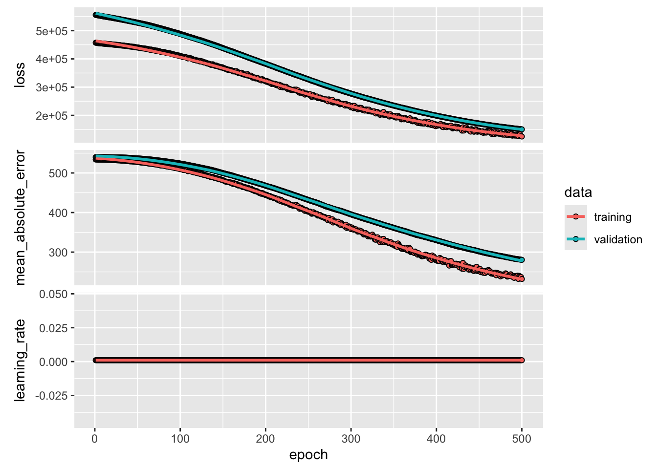 

plot(reg_history)

Figure 11.10: Training and validation MAE over epochs for the Hitters regression model. The gap between training and validation curves is a visual measure of overfitting — see Table 11.28.

11.11.3.6 Evaluate Against Benchmarks

npred   <- predict(reg_model, x[testid, ])

3/3 - 0s - 54ms/step

mae_nn  <- mean(abs(y[testid] - npred))

# Summary comparison — connects to @tbl-regression-metrics
tibble::tibble(
  Model = c("Linear Regression", "Lasso", "Neural Network (2-layer)"),
  MAE   = round(c(mae_lm, mae_lasso, mae_nn), 1)
) |>
  knitr::kable(caption = "Mean absolute error on the held-out test set for three models fitted to the `Hitters` salary data. {#tbl-reg-compare}")

Table 11.32: Mean absolute error on the held-out test set for three models fitted to the Hitters salary data.

Model	MAE
Linear Regression	254.7
Lasso	253.1
Neural Network (2-layer)	280.5

ImportantWhy does the NN lose to Lasso here?

The result in Table 11.32 is expected, not surprising. Three features of the Hitters data make it a poor fit for a neural network:

• Tiny \(n\). With only 175 training observations and 19 predictors, the NN has ~1,500 parameters to estimate from a handful of data points.
  • Lasso uses regularization to select a sparse subset of the 19 predictors; the NN has no such built-in parsimony.
  • The result is that the NN overfits the training data and generalizes poorly.
• Largely linear signal. Baseball salary is well-approximated by a linear combination of career statistics.
  • The non-linear interactions a NN is designed to exploit simply are not present in sufficient strength to justify the added model complexity.
• High irreducible noise. Salary negotiations involve factors (agent, market timing, team payroll constraints) that are not in the data.
  • When the noise floor is high, the NN’s extra flexibility fits noise rather than signal.

This is a deliberate first example: it establishes the baseline that a neural network is not automatically better than a regularized linear model.

• The next two examples test whether more data (\(n \approx 86{,}000\)) and genuinely non-linear signal change that conclusion.

---

11.11.4 Part 1b — Does More Data Always Help? NYC 311 Complaints

The Hitters result leaves open a natural question: is the NN’s poor performance simply a consequence of small \(n\)?

• This example tests that hypothesis with a much larger dataset (NYC 311 service requests (~86k rows)) to see whether scale alone is enough to flip the result.

NoteData

The two parquet files (nyc311_MANHATTAN_BRONX_2023-01.parquet, nyc311_MANHATTAN_BRONX_2023-07.parquet) contain all closed 311 complaints for Manhattan and the Bronx from January and July 2023 (~95,000 rows combined, zero nulls in key columns). They are read with arrow.

The January file is dominated by HEAT/HOT WATER complaints; July by Noise and Illegal Fireworks.

• The the seasonal contrast gives the model meaningful temporal signal to exploit.

The response variable is response_hours, the time from complaint creation to closure, which is pre-computed in the data.

11.11.4.1 Load and Combine Data

library(arrow)

jan <- read_parquet("data/nyc311_data/nyc311_MANHATTAN_BRONX_2023-01.parquet")
jul <- read_parquet("data/nyc311_data/nyc311_MANHATTAN_BRONX_2023-07.parquet")

raw311 <- bind_rows(jan, jul)
cat("Combined rows:", format(nrow(raw311), big.mark = ","), "\n")

Combined rows: 95,006 

11.11.4.2 Feature Engineering and Cleaning

The response is log-transformed to compress the heavy right tail (some complaints take weeks; most resolve within days).

• Categorical predictors are retained as factors and one-hot encoded in the next step.

df311 <- raw311 |>
  mutate(
    log_hrs        = log1p(response_hours),
    hour_of_day    = hour(created_date),
    day_of_week    = wday(created_date),
    month          = month(created_date),
    complaint_type = fct_lump_n(complaint_type, n = 20),
    agency         = fct_lump_n(agency,         n = 15),
    channel        = fct_lump_n(open_data_channel_type, n = 5)
  ) |>
  filter(
    response_hours > 0,
    response_hours < 24 * 30
  ) |>
  select(log_hrs, complaint_type, borough, agency,
         channel, hour_of_day, day_of_week, month) |>
  drop_na()

cat("Usable rows after filtering:", format(nrow(df311), big.mark = ","), "\n")

Usable rows after filtering: 86,180 

11.11.4.3 One-Hot Encode and Scale

The categorical predictors are one-hot encoded with model.matrix() (dropping the intercept column).

• Numeric predictors (hour_of_day, day_of_week, month) are range-scaled to \([0, 1]\) by dividing by their maximum, a simple scaling that preserves the cyclical spacing.

X311    <- model.matrix(log_hrs ~ ., data = df311)[, -1]

num_cols311 <- c("hour_of_day", "day_of_week", "month")
num_idx311  <- which(colnames(X311) %in% num_cols311)
X311[, num_idx311] <- apply(X311[, num_idx311], 2, \(v) v / max(v))

y311 <- df311$log_hrs
cat("Feature matrix:", nrow(X311), "rows x", ncol(X311), "columns\n")

Feature matrix: 86180 rows x 40 columns

NoteWhy One-Hot Encode Factors?

Neural networks require numeric input features, but variables such as borough, agency, and complaint_type are categorical factors stored as labels rather than numbers.

• One-hot encoding converts each category into a separate binary indicator column so the model can learn distinct weights for each category independently.

This avoids incorrectly imposing an artificial ordering on categories.

• For example, encoding boroughs as integers (Bronx = 1, Brooklyn = 2, etc.) would incorrectly imply numeric distance or rank relationships between categories that are purely nominal.

In R, model.matrix() provides a convenient and efficient way to automatically convert factors into a numeric design matrix suitable for machine learning frameworks such as Keras and TensorFlow.

• This preprocessing step is standard for neural networks and many other predictive modeling approaches using tabular data.

11.11.4.4 Train / Test Split

Set the random number seed and split 80-20.

set.seed(42)
tensorflow::set_random_seed(42L)

n311   <- nrow(X311)
idx311 <- sample(n311, size = floor(0.8 * n311))

x311_tr <- X311[idx311, ];   y311_tr <- y311[idx311]
x311_te <- X311[-idx311, ];  y311_te <- y311[-idx311]

cat("Train:", format(nrow(x311_tr), big.mark = ","),
    "| Test:", format(nrow(x311_te), big.mark = ","), "\n")

Train: 68,944 | Test: 17,236 

11.11.4.5 Baseline 1 — Linear Regression

lm311      <- lm(y311_tr ~ x311_tr)
pred_lm311 <- predict(lm311, as.data.frame(x311_te))
mae_lm311  <- mean(abs(pred_lm311 - y311_te))
cat("Linear regression MAE (log-hrs):", round(mae_lm311, 4), "\n")

Linear regression MAE (log-hrs): 2.1727 

11.11.4.6 Baseline 2 — Lasso

lasso311     <- cv.glmnet(x311_tr, y311_tr, alpha = 1)
pred_lasso311 <- predict(lasso311, x311_te, s = "lambda.min")
mae_lasso311 <- mean(abs(pred_lasso311 - y311_te))
cat("Lasso MAE (log-hrs):", round(mae_lasso311, 4), "\n")

Lasso MAE (log-hrs): 0.7194 

11.11.4.7 Neural Network

With ~70k training observations and 40 features, a wider architecture with batch normalization is appropriate, the opposite of the Hitters case.

NoteBatch normalization is back

With batch size 256 and ~70k training rows there are ≈ 270 batches per epoch , enough for stable batch norm running statistics.

• Compare this to the Hitters model where only ~5–6 batches per epoch made batch norm unreliable.

# Input: one-hot encoded + scaled predictors (p columns)
# L1: 128 nodes — wide enough to capture complaint_type x agency interactions
# L2:  64 nodes — compress
# L3:  32 nodes — compress further
# Output: 1 node, linear (regression)
p311 <- ncol(x311_tr)

nn311 <- keras_model_sequential(name = "nyc311_regression") |>
  layer_dense(units = 128, activation = "relu",
              input_shape = p311, name = "hidden_1") |>
  layer_batch_normalization(name = "bn_1") |>
  layer_dropout(rate = 0.3, name = "dropout_1") |>
  layer_dense(units = 64,  activation = "relu", name = "hidden_2") |>
  layer_batch_normalization(name = "bn_2") |>
  layer_dropout(rate = 0.2, name = "dropout_2") |>
  layer_dense(units = 32,  activation = "relu", name = "hidden_3") |>
  layer_dropout(rate = 0.1, name = "dropout_3") |>
  layer_dense(units = 1, name = "output")

summary(nn311)

Model: "nyc311_regression"
┏━━━━━━━━━━━━━━━━━━━━━━━━━━━━━━━┳━━━━━━━━━━━━━━━━━━━━━━━━┳━━━━━━━━━━━━━┳━━━━━━━┓
┃ Layer (type)                  ┃ Output Shape           ┃     Param # ┃ Trai… ┃
┡━━━━━━━━━━━━━━━━━━━━━━━━━━━━━━━╇━━━━━━━━━━━━━━━━━━━━━━━━╇━━━━━━━━━━━━━╇━━━━━━━┩
│ hidden_1 (Dense)              │ (None, 128)            │       5,248 │   Y   │
├───────────────────────────────┼────────────────────────┼─────────────┼───────┤
│ bn_1 (BatchNormalization)     │ (None, 128)            │         512 │   Y   │
├───────────────────────────────┼────────────────────────┼─────────────┼───────┤
│ dropout_1 (Dropout)           │ (None, 128)            │           0 │   -   │
├───────────────────────────────┼────────────────────────┼─────────────┼───────┤
│ hidden_2 (Dense)              │ (None, 64)             │       8,256 │   Y   │
├───────────────────────────────┼────────────────────────┼─────────────┼───────┤
│ bn_2 (BatchNormalization)     │ (None, 64)             │         256 │   Y   │
├───────────────────────────────┼────────────────────────┼─────────────┼───────┤
│ dropout_2 (Dropout)           │ (None, 64)             │           0 │   -   │
├───────────────────────────────┼────────────────────────┼─────────────┼───────┤
│ hidden_3 (Dense)              │ (None, 32)             │       2,080 │   Y   │
├───────────────────────────────┼────────────────────────┼─────────────┼───────┤
│ dropout_3 (Dropout)           │ (None, 32)             │           0 │   -   │
├───────────────────────────────┼────────────────────────┼─────────────┼───────┤
│ output (Dense)                │ (None, 1)              │          33 │   Y   │
└───────────────────────────────┴────────────────────────┴─────────────┴───────┘
 Total params: 16,385 (64.00 KB)
 Trainable params: 16,001 (62.50 KB)
 Non-trainable params: 384 (1.50 KB)

Compile the model

keras3::compile(nn311,
  optimizer = optimizer_adam(learning_rate = 1e-3),
  loss      = "mae",
  metrics   = list("mean_absolute_error")
)

Check if the model exists and if not fit the model and save the results as well as a plot of the training history.

model_path_311 <- "models/nn311.keras"

if (file.exists(model_path_311)) {
  nn311      <- load_model(model_path_311)
  history311 <- NULL
  cat("Loaded saved model from", model_path_311, "\n")
} else {
  dir.create("models", showWarnings = FALSE)
  history311 <- nn311 |> fit(
    x311_tr, y311_tr,
    epochs           = 30,
    batch_size       = 256,
    validation_split = 0.15,
    verbose          = 0
  )
  save_model(nn311, model_path_311)
  png("models/nn311_history.png", width = 800, height = 500)
  plot(history311)
  dev.off()
  cat("Trained and saved model to", model_path_311, "\n")
}

11.11.4.8 Training History

knitr::include_graphics("models/nn311_history.png")

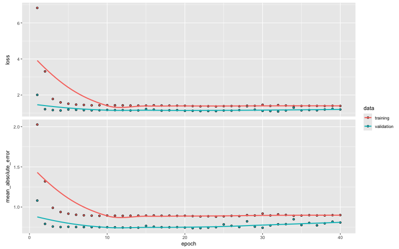
Figure 11.11: Training and validation MAE (log-hours) over epochs for the NYC 311 neural network. The x-axis extends to the maximum epochs specified (30) regardless of when training ended — default behaviour of plot.keras_training_history(). Both curves converge and track closely, indicating the model is not overfitting.

11.11.4.9 Evaluate on the Test Set

mae_nn311 <- nn311 |>
  evaluate(x311_te, y311_te, verbose = 0) |>
  (`[[`)("mean_absolute_error")

cat("Neural network MAE (log-hrs):", round(mae_nn311, 4), "\n")

Neural network MAE (log-hrs): 0.7459 

11.11.4.10 Compare All Three Models

tibble::tibble(
  Model          = c("Linear Regression", "Lasso", "Neural Network (3-layer)"),
  `MAE (log-hrs)` = round(c(mae_lm311, mae_lasso311, mae_nn311), 4)
) |>
  knitr::kable(
    caption = "Mean absolute error on the held-out test set for three models
    predicting log(resolution hours) on NYC 311 complaints.
    {#tbl-nyc311-compare}"
  )

Table 11.33: Mean absolute error on the held-out test set for three models predicting log(resolution hours) on NYC 311 complaints. {#tbl-nyc311-compare}

Model	MAE (log-hrs)
Linear Regression	2.1727
Lasso	0.7194
Neural Network (3-layer)	0.7459

ImportantLarge \(n\) alone does not guarantee a neural network win

Table 11.33 shows Lasso beating the NN despite ~86k training rows.

• The reason is signal structure, not sample size.

Simple linear models expose the problem. Three nested regressions on log_hrs:

Predictors	\(R^2\)
complaint_type only	0.642
+ agency	0.745
+ agency + month	0.747

74.5% of the variance in resolution time is explained by just two additive main effects.

• The residual variance is largely irreducible noise within complaint type \(\times\) agency cells.
• There is almost nothing left for the NN’s interaction-learning to exploit.
• Lasso finds the optimal combination of those main effects and stops, correctly.

The lesson: large \(n\) is a necessary condition for a NN win on tabular data, not a sufficient one.

• The signal must be genuinely non-linear.
• The next example demonstrates a dataset where that condition is met.

---

11.11.5 Part 1c — When the Neural Network Wins: NYC Taxi Fare Amount

NYC yellow taxi trips demonstrate genuine non-linearity: metered fare amount depends on the interaction of pickup location, dropoff location, trip distance, time of day, and day of week in ways no additive linear model can represent without explicit engineering.

• New York’s pricing structure contains hard discontinuities
  • flat-rate airport trips,
  • congestion-zone surcharges, and
  • distance thresholds

A NN can learn implicitly from raw zone IDs and distance, while Lasso must approximate them linearly.

NoteData

NYC TLC trip records are available as monthly parquet files from the TLC Trip Record Data page.

• The January 2023 yellow taxi parquet (~3M rows) is used here.
• We sample 300,000 trips to give the NN enough zone-pair coverage to detect the pricing discontinuities.
• The parquet is read directly from the TLC CloudFront CDN so no local download is needed.

We predict the metered fare (fare_amount), the base clock fare before surcharges, tips, or tolls.

• Excluding congestion_surcharge and airport_fee from the feature set is deliberate;if included, those additive terms hand Lasso a near-perfect linear signal and eliminate the NN’s advantage.
• The non-linearity we want the NN to discover is the zone-pair pricing structure embedded in trip_distance, PULocationID, and DOLocationID.

11.11.5.1 Load and Prepare Data

taxi_raw <- arrow::read_parquet(
  "https://d37ci6vzurychx.cloudfront.net/trip-data/yellow_tripdata_2023-01.parquet"
)

cat("Raw rows:", format(nrow(taxi_raw), big.mark = ","), "\n")

Raw rows: 3,066,766 

Set the random number seed and sample the filtered data

set.seed(42)
tensorflow::set_random_seed(42L)

taxi_fare300 <- taxi_raw |>
  mutate(
    duration_min = as.numeric(
      difftime(tpep_dropoff_datetime, tpep_pickup_datetime, units = "mins")
    ),
    hour_of_day = as.numeric(hour(tpep_pickup_datetime)),
    day_of_week = as.numeric(wday(tpep_pickup_datetime))
  ) |>
  filter(
    duration_min    >   1, duration_min    < 120,
    trip_distance   > 0.1, trip_distance   <  50,
    passenger_count >=  1,
    fare_amount     > 2.5, fare_amount     < 200,
    PULocationID    <=  263,
    DOLocationID    <=  263
  ) |>
  select(fare_amount, trip_distance, passenger_count,
         PULocationID, DOLocationID,
         hour_of_day, day_of_week, duration_min) |>
  drop_na() |>
  slice_sample(n = 300000)

cat("Usable rows:", format(nrow(taxi_fare300), big.mark = ","), "\n")

Usable rows: 300,000 

cat("Features:   ", ncol(taxi_fare300) - 1, "(excl. outcome)\n")

Features:    7 (excl. outcome)

NoteWhy Apply These Filters to NYC Taxi Data?

Real-world transportation data often contains invalid, incomplete, or highly unusual records caused by GPS failures, meter errors, cancelled trips, test records, or data-entry problems.

• These filters remove observations that are unlikely to represent normal taxi rides and help stabilize the analysis.
  • Trips shorter than one minute or longer than two hours are often errors or atypical events.
  • Distances under 0.1 miles or above 50 miles are similarly suspicious for standard NYC taxi trips.
  • Filtering fare amounts removes negative, zero, or implausibly large charges that can distort model training.
  • Requiring at least one passenger excludes invalid records,
  • Restricting pickup and dropoff location IDs to the valid NYC Taxi & Limousine Commission zone range ensures that only recognized taxi zones are included.

These filters improve data quality, reduce the influence of extreme outliers, and produce more stable and interpretable predictive models.

11.11.5.2 Scale Features and Split

Scale first then split the data into 80/20

x300 <- taxi_fare300 |>
  select(-fare_amount) |>
  as.matrix()

x300_means <- colMeans(x300)
x300_sds   <- apply(x300, 2, sd)
y300        <- taxi_fare300$fare_amount

set.seed(42)
idx300      <- sample(nrow(x300), floor(0.8 * nrow(x300)))
x300_tr     <- x300[idx300, ];   y300_tr <- y300[idx300]
x300_te     <- x300[-idx300, ];  y300_te <- y300[-idx300]

x300_tr_sc  <- scale(x300_tr, center = x300_means, scale = x300_sds)
x300_te_sc  <- scale(x300_te, center = x300_means, scale = x300_sds)

cat("Features:", ncol(x300),
    "| Train:", format(nrow(x300_tr), big.mark = ","),
    "| Test:",  format(nrow(x300_te), big.mark = ","), "\n")

Features: 7 | Train: 240,000 | Test: 60,000 

11.11.5.3 Baseline — Lasso

lasso300      <- cv.glmnet(x300_tr_sc, y300_tr, alpha = 1)
pred_lasso300 <- predict(lasso300, x300_te_sc, s = "lambda.min")
mae_lasso300  <- mean(abs(pred_lasso300 - y300_te))
cat("Lasso MAE (dollars):", round(mae_lasso300, 2), "\n")

Lasso MAE (dollars): 1.19 

11.11.5.4 Neural Network — 3-Layer, MAE Loss

Define the network.

nn300 <- keras_model_sequential(name = "taxi_fare") |>
  layer_dense(units = 256, activation = "relu", input_shape = 7L) |>
  layer_dropout(rate = 0.1) |>
  layer_dense(units = 128, activation = "relu") |>
  layer_dropout(rate = 0.1) |>
  layer_dense(units = 64,  activation = "relu") |>
  layer_dense(units = 1)

keras3::compile(nn300,
  optimizer = optimizer_adam(learning_rate = 1e-3),
  loss      = "mae"
)

Check if the model exists and if not fit the model and save the results and the training history plot.

model_path_300 <- "models/nn300.keras"

if (file.exists(model_path_300)) {
  nn300      <- load_model(model_path_300)
  history300 <- NULL
  cat("Loaded saved model from", model_path_300, "\n")
} else {
  dir.create("models", showWarnings = FALSE)
  history300 <- nn300 |> fit(
    x300_tr_sc, y300_tr,
    epochs           = 30,
    batch_size       = 512,
    validation_split = 0.1,
    callbacks = list(
      callback_early_stopping(monitor          = "val_loss",
                              patience         = 10,
                              restore_best_weights = TRUE)
    ),
    verbose = 0
  )
  save_model(nn300, model_path_300)
  png("models/nn300_history.png", width = 800, height = 500)
  plot(history300)
  dev.off()
  cat("Trained and saved model to", model_path_300, "\n")
}

11.11.5.5 Training History

knitr::include_graphics("models/nn300_history.png")

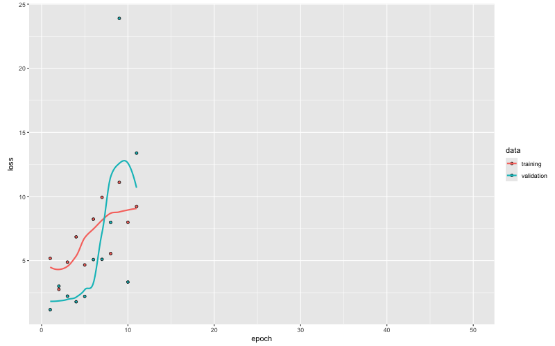
Figure 11.12: Training and validation MAE (dollars) over epochs. The x-axis extends to the maximum epochs specified (30) regardless of when early stopping triggered — this is the default behaviour of plot.keras_training_history(). Active training ended at epoch 11 (where the curves terminate); the flat region to the right is empty axis space, not stagnation. Best weights from epoch 11 are restored automatically by restore_best_weights = TRUE.

11.11.5.6 Evaluate on the Test Set

pred_nn300 <- predict(nn300, x300_te_sc, verbose = 0)
mae_nn300  <- mean(abs(pred_nn300 - y300_te))

cat("Lasso MAE (dollars):", round(mae_lasso300, 2), "\n")

Lasso MAE (dollars): 1.19 

cat("NN MAE    (dollars):", round(mae_nn300,    2), "\n")

NN MAE    (dollars): 1.17 

cat("Improvement:        ", round((1 - mae_nn300 / mae_lasso300) * 100, 1), "%\n")

Improvement:         1.5 %

11.11.5.7 Compare Models

tibble::tibble(
  Model           = c("Lasso", "Neural Network (3-layer)"),
  `MAE (dollars)` = round(c(mae_lasso300, mae_nn300), 2)
) |>
  knitr::kable(
    caption = "Mean absolute error predicting NYC yellow taxi metered fare (300k trips).
    {#tbl-taxi-compare}"
  )

Table 11.34: Mean absolute error predicting NYC yellow taxi metered fare (300k trips). {#tbl-taxi-compare}

Model	MAE (dollars)
Lasso	1.19
Neural Network (3-layer)	1.17

ImportantWhat the three examples teach together

Dataset	\(n\) (train)	Signal structure	Winner
Hitters salary	~175	Linear, low-dim	Lasso
NYC 311 resolution time	~68k	Additive main effects	Lasso
NYC taxi fare amount	~240k	Non-linear zone-pair pricing discontinuities	NN

The taxi fare data has the right conditions for a NN win:

• Pricing discontinuities. JFK and LaGuardia trips carry flat-rate surcharges; Manhattan’s congestion zone creates a step-change in effective fare per mile.
  • These are threshold effects that Lasso can only approximate linearly; the NN’s ReLU activations model thresholds naturally.
• Zone-pair interactions. The fare from zone 132 (JFK) to zone 161 (Midtown) is not the sum of a pickup effect and a dropoff effect so the combination matters.
• The NN learns these joint effects in its hidden layers; Lasso would need an explicit column for every zone pair (\(263 \times 263 \approx 69{,}000\) columns).
• Structured residual variance. Variance unexplained by linear main effects is predictable from zone-pair combinations; it is signal, not noise.

Core principle: a neural network wins when

• (1) \(n\) is large enough to estimate parameters reliably, and
• (2) the outcome depends on non-linear combinations of inputs too complex to engineer explicitly.

WarningMore data does not always favour the NN

It is tempting to assume that scaling from 300k to 3M rows would widen the NN’s lead further. For this dataset the opposite may be true.

• At very large \(n\), Lasso gains access to enough observations to estimate zone-pair effects precisely, effectively recovering the pricing structure without non-linear activations.
• The NN’s advantage comes partly from generalizing across sparse zone pairs; once every zone pair is densely observed, that advantage shrinks.

More fundamentally, the metered fare is close to linear in trip distance within each zone pair: it follows the TLC rate card (a fixed flag-drop charge plus a per-mile rate).

• The non-linearity is real but shallow.
• When \(n\) grows large enough for Lasso to fit each zone’s intercept shift accurately, the linear model converges toward the same solution and the MAE gap closes.

The lesson: the NN vs. Lasso contest depends on the depth of non-linearity relative to \(n\). Shallow non-linearity + very large \(n\) often tips back toward the simpler model.

---

11.11.6 Part 2 — Classification: Movie Hit or Flop

This example connects directly to Case B in Section 11.4. We simulate a movie dataset with features analogous to the worked example (budget, genre indicators, cast score, etc.) and predict whether a movie is a Hit (top tercile box office) or a Flop (bottom tercile).

Note

A real version of this analysis could use publicly available data from The Numbers or Box Office Mojo.

• The simulated data here is structured to match the worked example exactly so you can trace the computations from Section 11.4 through to the fitted model.

11.11.6.1 Simulate the Data

set.seed(42)
n_movies <- 500

movies <- tibble::tibble(
  budget_m      = runif(n_movies, 5, 200),         # $M production budget
  cast_score    = runif(n_movies, 0, 10),           # aggregate star power score
  sequel        = rbinom(n_movies, 1, 0.3),         # is it a sequel?
  genre_action  = rbinom(n_movies, 1, 0.25),
  genre_comedy  = rbinom(n_movies, 1, 0.20),
  marketing_m   = runif(n_movies, 1, 80)            # $M marketing spend
) |>
  dplyr::mutate(
    # True log-revenue depends on features + noise
    log_revenue = 0.8 * log(budget_m) +
                  0.5 * cast_score +
                  0.4 * sequel +
                  0.3 * genre_action +
                  0.2 * genre_comedy +
                  0.3 * log(marketing_m) +
                  rnorm(n_movies, sd = 0.8),
    # Hit = top tercile; Flop = bottom tercile; middle dropped for clarity
    tercile = dplyr::ntile(log_revenue, 3),
    hit     = dplyr::case_when(
      tercile == 3 ~ 1L,
      tercile == 1 ~ 0L
    )
  ) |>
  dplyr::filter(!is.na(hit))

cat("Dataset:", nrow(movies), "movies |",
    sum(movies$hit), "Hits |", sum(1 - movies$hit), "Flops\n")

Dataset: 333 movies | 166 Hits | 167 Flops

11.11.6.2 Prepare Features and Split

Split on 75:25.

tensorflow::set_random_seed(42L)

# Feature matrix — scale for gradient descent stability (@eq-xavier)
x_mov <- scale(as.matrix(
  movies[, c("budget_m", "cast_score", "sequel",
             "genre_action", "genre_comedy", "marketing_m")]
))
y_mov <- movies$hit

set.seed(42)
ntest_mov  <- trunc(nrow(movies) * 0.25)
testid_mov <- sample(seq_len(nrow(movies)), ntest_mov)

cat("Training:", nrow(movies) - ntest_mov,
    "| Test:", ntest_mov,
    "| Features:", ncol(x_mov), "\n")

Training: 250 | Test: 83 | Features: 6 

11.11.6.3 Baseline — Logistic Regression (Lasso)

Use {proc} to get the AUC values.

lasso_mov      <- cv.glmnet(
  x_mov[-testid_mov, ], y_mov[-testid_mov],
  alpha  = 1,
  family = "binomial"
)

prob_lasso_mov <- predict(lasso_mov, x_mov[testid_mov, ],
                          s = "lambda.min", type = "response")
pred_lasso_mov <- as.integer(prob_lasso_mov > 0.5)
acc_lasso_mov  <- mean(pred_lasso_mov == y_mov[testid_mov])

roc_lasso_mov  <- pROC::roc(y_mov[testid_mov], as.vector(prob_lasso_mov),
                             quiet = TRUE)
auc_lasso_mov  <- as.numeric(pROC::auc(roc_lasso_mov))

cat(sprintf("Logistic Lasso -- Accuracy: %.1f%%  AUC: %.3f\n",
            acc_lasso_mov * 100, auc_lasso_mov))

Logistic Lasso -- Accuracy: 91.6%  AUC: 0.972

11.11.6.4 Define the Classification Model Architecture

Specify the model design and compile the model.

# Architecture: 5 inputs → 32 → 16 → 1 (sigmoid output)
# - Sigmoid output gives P(Hit) ∈ (0, 1) — see @eq-sigmoid
# - Loss: binary cross-entropy — see @eq-cross entropy-loss
# - For multiclass (M > 2): use softmax + categorical_crossentropy
#   (@eq-softmax, @eq-total-loss-classification)

# keras3: input_shape declared on the constructor — not via layer_input()
clf_model <- keras_model_sequential(
  name        = "movie_classification",
  input_shape = ncol(x_mov)         # number of movie feature inputs
) |>
  layer_dense(units = 32, activation = "relu",
              name = "hidden_1") |>
  layer_batch_normalization(name = "bn_1") |>
  layer_dropout(rate = 0.3, name = "dropout_1") |>
  layer_dense(units = 16, activation = "relu",
              name = "hidden_2") |>
  layer_dropout(rate = 0.2, name = "dropout_2") |>
  layer_dense(units = 1, activation = "sigmoid",
              name = "output")         # P(Hit) — see @eq-sigmoid

keras3::compile(clf_model,
 
    optimizer = optimizer_adam(learning_rate = 1e-3),
    loss      = "binary_crossentropy",   # @eq-total-loss-classification
    metrics   = list("accuracy", metric_auc(name = "auc"))
  )

summary(clf_model)

Model: "movie_classification"
┏━━━━━━━━━━━━━━━━━━━━━━━━━━━━━━━┳━━━━━━━━━━━━━━━━━━━━━━━━┳━━━━━━━━━━━━━┳━━━━━━━┓
┃ Layer (type)                  ┃ Output Shape           ┃     Param # ┃ Trai… ┃
┡━━━━━━━━━━━━━━━━━━━━━━━━━━━━━━━╇━━━━━━━━━━━━━━━━━━━━━━━━╇━━━━━━━━━━━━━╇━━━━━━━┩
│ hidden_1 (Dense)              │ (None, 32)             │         224 │   Y   │
├───────────────────────────────┼────────────────────────┼─────────────┼───────┤
│ bn_1 (BatchNormalization)     │ (None, 32)             │         128 │   Y   │
├───────────────────────────────┼────────────────────────┼─────────────┼───────┤
│ dropout_1 (Dropout)           │ (None, 32)             │           0 │   -   │
├───────────────────────────────┼────────────────────────┼─────────────┼───────┤
│ hidden_2 (Dense)              │ (None, 16)             │         528 │   Y   │
├───────────────────────────────┼────────────────────────┼─────────────┼───────┤
│ dropout_2 (Dropout)           │ (None, 16)             │           0 │   -   │
├───────────────────────────────┼────────────────────────┼─────────────┼───────┤
│ output (Dense)                │ (None, 1)              │          17 │   Y   │
└───────────────────────────────┴────────────────────────┴─────────────┴───────┘
 Total params: 897 (3.50 KB)
 Trainable params: 833 (3.25 KB)
 Non-trainable params: 64 (256.00 B)

11.11.6.5 Fit with Early Stopping

callbacks_clf <- list(
  callback_early_stopping(
    monitor              = "val_auc",
    mode                 = "max",   # AUC should increase
    patience             = 25,
    restore_best_weights = TRUE
  )
)

clf_history <- clf_model |>
  fit(
    x_mov[-testid_mov, ], y_mov[-testid_mov],
    epochs          = 300,
    batch_size      = 32,
    validation_data = list(x_mov[testid_mov, ], y_mov[testid_mov]),
    callbacks       = callbacks_clf,
    verbose         = 0
  )

cat("Stopped at epoch:", length(clf_history$metrics$loss), "\n")

Stopped at epoch: 74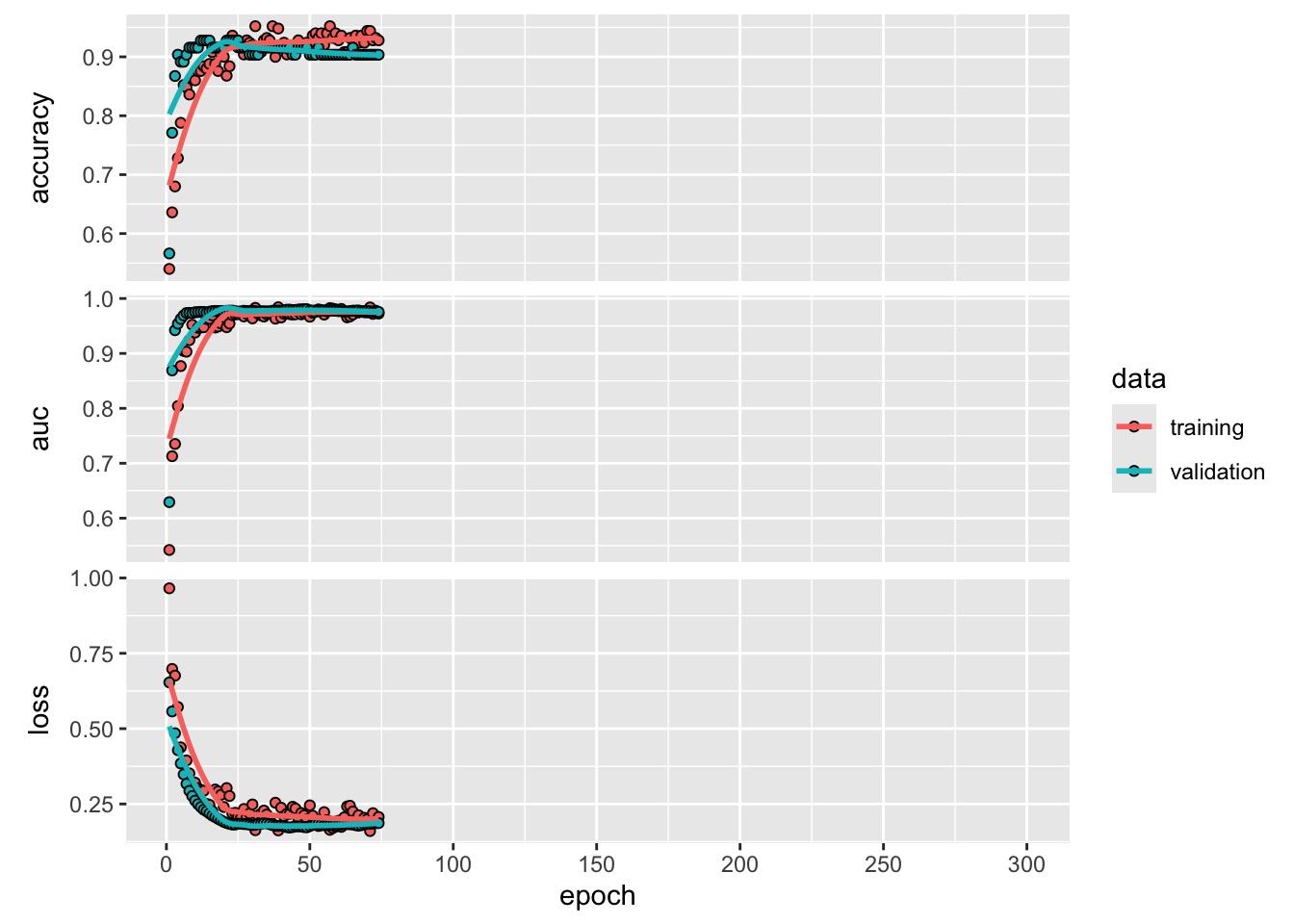 

plot(clf_history)

11.11.6.6 Evaluate the Classification Model

# Predicted probabilities -> class predictions at 0.5 threshold
prob_hit   <- predict(clf_model, x_mov[testid_mov, ], verbose = 0)
pred_class <- as.integer(prob_hit > 0.5)
true_class <- y_mov[testid_mov]

# Confusion matrix
conf_mat <- table(
  Predicted = factor(pred_class, labels = c("Flop", "Hit")),
  Actual    = factor(true_class,  labels = c("Flop", "Hit"))
)
print(conf_mat)

         Actual
Predicted Flop Hit
     Flop   36   2
     Hit     5  40

# NN metrics
acc_nn_mov <- mean(pred_class == true_class)
auc_nn_mov <- clf_model |>
  evaluate(x_mov[testid_mov, ], y_mov[testid_mov], verbose = 0)

# Side-by-side comparison with Lasso baseline
tibble::tibble(
  Model    = c("Logistic Regression (Lasso)", "Neural Network (3-layer)"),
  Accuracy = sprintf("%.1f%%", c(acc_lasso_mov, acc_nn_mov) * 100),
  AUC      = round(c(auc_lasso_mov, auc_nn_mov[["auc"]]), 3)
) |>
  knitr::kable(
    caption = "Classification performance predicting movie Hit vs. Flop
    (simulated data, 25% test set). {#tbl-movie-compare}"
  )

Table 11.35: Classification performance predicting movie Hit vs. Flop (simulated data, 25% test set).

Model	Accuracy	AUC
Logistic Regression (Lasso)	91.6%	0.972
Neural Network (3-layer)	91.6%	0.981

NoteInterpreting the Similar Performance of the Lasso and Neural Network

The neural network achieves only a slightly lower mean absolute error (MAE) than the lasso model (\(1.17\) versus \(1.19\)).

• This suggests that much of the predictive structure in NYC taxi fares is already well explained by relatively simple and approximately linear relationships among variables such as trip distance, trip duration, pickup/dropoff zones, and passenger count.

Taxi fares are heavily determined by a rule-based pricing system established by the NYC Taxi & Limousine Commission, meaning the underlying relationship between predictors and fare is largely additive and structured.

• As a result, a regularized linear model such as lasso can capture most of the signal effectively.

The neural network may still provide a modest improvement by learning nonlinear interactions and localized effects that the linear model cannot easily represent, such as congestion patterns, geographic interactions between neighborhoods, or nonlinear fare behavior at very short or very long trips.

• However, because the fare-generation process itself is relatively systematic, the advantage of a more flexible deep learning model remains limited in this setting.

---

11.11.7 Comparing the Two Tasks

The two models illustrate how the same architectural decisions from Section 11.4 and Table 11.1 play out differently depending on the task:

Design differences between the regression and classification labs.

Design choice	Regression (Hitters)	Classification (Movies)
Output activation	None (linear)	Sigmoid — Equation 11.5
Loss function	MSE — Equation 11.29	Binary cross-entropy — Equation 11.33
Monitoring metric	MAE	AUC (Table 11.26)
Early stopping monitor	val_mean_absolute_error	val_auc (mode = max)
Output interpretation	Predicted salary ($)	\(\hat{P}(\text{Hit})\)

The hidden layers, batch normalization, dropout, Adam optimizer, and early stopping callbacks are identical in both.

• This shows the core training machinery from Section 11.4 generalizes across task types.
• Only the output layer and loss function change.

11.12 Experimenting with Google Colab

Google Colab (https://colab.research.google.com/ ) provides a convenient browser-based environment for experimenting with neural networks and modern AI workflows without requiring you to install Python, TensorFlow, or other machine learning libraries on your personal computers.

• Colab notebooks run entirely in the browser and provide access to preconfigured Python environments with scientific computing and deep learning tools already installed.
• This allows one to focus on the conceptual aspects of neural networks such as forward passes, backpropagation, optimization, and hyperparameter tuning, rather than spending time debugging software installations or configuring local environments.

You can download a Colab Jupyter notebook at https://github.com/AU-datascience/data/blob/main/427-627/colab_nn_examples.ipynb and upload it into Google Colab to use as an interactive “playground” for experimenting with neural networks on small datasets.

• The noetbook is in written in Python but you can experiment by changing the cells that define the hyperparameters for the networks included as examples.
• You can can modify network architectures, activation functions, learning rates, and training parameters and immediately observe how those changes affect model performance.
• This environment is especially useful for comparing neural networks to more traditional statistical and machine learning models such as logistic regression or lasso regression, helping yiou to understand both the strengths and limitations of deep learning methods.

11.13 Convolutional Neural Networks (CNN)

Convolutional Neural Networks (CNNs) are a special type of neural network architecture designed for processing grid-like data, particularly images.

• CNNs excel at tasks such as image classification, object detection, and facial recognition by automatically learning useful visual features from pixel data.
• Unlike fully connected neural networks, where every neuron connects to every input value, CNNs apply learned filters (also called kernels) to small overlapping regions of the input image.
• As the filter moves across the image, the network computes weighted sums of the pixel values within each region using the learned filter parameters.
• The resulting values are passed through a nonlinear activation function, allowing the network to learn increasingly complex patterns and features.
• In mathematics, this sliding weighted-combination operation is called a Convolution, which gives Convolutional Neural Networks their name.

Figure 11.13 shows a typical CNN such as might be used for image classification (cat or dog).

Figure 11.13: Architecture of a typical Convolutional Neural Network (CNN) for image classification. From left to right: the raw pixel input image; alternating convolutional layers (which apply learned filters to detect local features) and pooling layers (which downsample the feature maps); flattening to a 1-D vector; fully connected dense layers; and a final softmax output layer producing class probabilities (e.g. cat vs. dog).

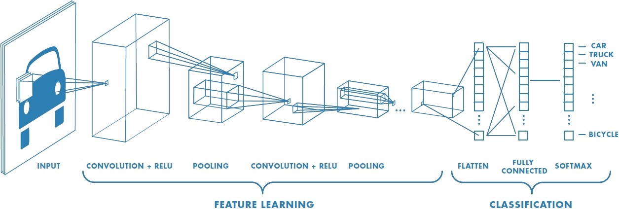
11.13.1 Input Layer has Raw Pixel Data

On the left of Figure 11.13 is the input layer.

Every CNN begins with an input layer that takes in the image as a multi-dimensional array of pixel values.

• For a color image, this typically includes three channels, red, green, and blue, resulting in a 3D input tensor (height × width × channels).
• The numerical values represent the intensity of each pixel.

11.13.2 Convolutional Layers for Feature Detectors

The next major component of a CNN is a convolutional layer, and CNNs often contain several such layers stacked together.

• A convolutional layer applies small, trainable filters (or kernels) that scan across the image to detect patterns and features.
• Each kernel performs an element-wise multiplication between the filter’s weights and a small region of the input image (for example, a \(3 \times 3\) patch of pixels).
• The resulting values are summed to produce a single activation value, which becomes one entry in the resulting feature map.
• The filter then moves across the image by a fixed number of pixels (called the stride) and repeats the process across the width and then height of the input.
• This continues until the filter has covered the entire image, producing a feature map: a 2D grid in which each value represents the strength or presence of a learned pattern at a particular location.

Key properties:

• Local connectivity: Filters examine local regions, preserving spatial relationships.
• Weight sharing: Each filter uses the same weights across the image, reducing model complexity.
• Depth: Multiple filters can be applied in a single convolutional layer, capturing various patterns simultaneously.

Early convolutional layers detect simple features like edges or colors; deeper layers detect more abstract concepts like shapes or object parts as shown in Figure 11.14.

Figure 11.14: Sample convolution operations and learned filters in a CNN. Early-layer filters (top row) respond to low-level features such as oriented edges, colour gradients, and corners. Deeper-layer filters (lower rows) respond to increasingly complex patterns such as textures, object parts, and whole shapes, illustrating the hierarchical feature-learning that makes CNNs effective for image tasks.

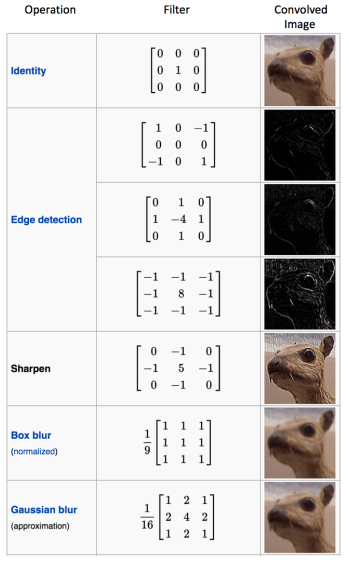
11.13.3 Activation Functions enable Non-Linearity

After each convolution operation, an activation function, usually ReLU, is used to introduce non-linearity by zeroing out negative values:

• This allows the network to model complex patterns and relationships that simple linear transformations cannot.

11.13.4 Pooling Layers Reduce the Dimensions of the Network

Next come pooling layers, which reduce the spatial dimensions of the feature maps.

• The most common pooling operation is “max pooling”, which slides a small window (e.g., 2×2) over the feature map and takes the maximum value in each region.
• This step simplifies the data, makes the network more computationally efficient, and introduces a level of translation invariance.

Key benefits:

• Reduces the number of parameters.
• Controls overfitting.
• Preserves the most important features while discarding minor variations.

Pooling doesn’t alter the number of feature maps; it just compresses them.

11.13.5 Stacking Multiple Layers Enables Hierarchical Learning about Image Features

CNNs often stack multiple convolutional and pooling layers to learn a hierarchy of features in the image as in Figure 11.13:

• Shallow layers detect low-level features like edges and corners.
• Intermediate layers detect textures, patterns, and shapes.
• Deep layers capture high-level features and object parts.

This layered approach is what gives CNNs their strength in capturing complex patterns in images while reducing computations.

11.13.6 Fully-Connected Layers are then Used for Classification

After the final convolutional and pooling layers, the high-level feature maps are flattened into a single vector and passed into one or more fully-connected layers.

• These layers act like a traditional neural network, using the learned features to predict a class label or probability distribution over multiple categories (e.g., Dog, Cat, Tiger, Lion).

11.13.7 Output Layer

The final layer is often a softmax classifier (for multi-class classification), which outputs a probability score for each class.

• The highest score determines the predicted category of the image.

NoteKernels in CNNs vs. SVMs

Note that kernels in CNNs are not the same as kernels in Support Vector Machines (SVMs):

• CNN kernels are learnable filters used to detect spatial patterns directly from input data.
• SVM kernels are mathematical functions (like polynomial) used to project data into higher-dimensional spaces to find separating boundaries.

While they share a name, they serve entirely different purposes in their respective algorithms.

CNNs are powerful for grid data because they combine:

• Local feature detection (via convolution),
• Efficient dimensionality reduction (via pooling),
• Non-linear transformations (via activation functions),
• and final classification (via fully connected layers).

This architecture allows them to automatically learn meaningful features and make accurate predictions from raw image data, without the need for manual feature engineering.

11.14 Transfer Learning and Pre-trained Models

11.14.1 Why Training from Scratch Is Rare

Training a network from scratch, initializing random weights (Equation 11.22) and running gradient descent (Equation 11.35) until convergence, is the process described throughout this chapter.

In practice, for most real-world problems in 2026, nobody does this.

The reason is scale.

• A frontier model like GPT-4 or Llama 3 has already consumed more text, images, or audio than any single organization could afford to process again.
• Its weight matrices (Equation 11.45) encode an enormous amount of general knowledge about language, visual structure, or domain reasoning.
• Starting from random weights throws all of that away.

Instead, practitioners use one of three strategies, in increasing order of cost:

11.14.2 Three Strategies for Using Pre-Trained Models

11.14.2.1 Strategy 1 — Feature Extraction (freeze and predict)

Take a pre-trained model, remove its output layer, and treat the activations of the final hidden layer as a fixed feature vector.

• Train only a new output layer on your data.
• The pre-trained weights are frozen; they receive no gradient updates (Equation 11.35 is not applied to them).

Characteristics:

• Cheapest: only the output layer parameters are learned.
• Works well when your data is small and similar to the pre-training domain.
• Example: use ResNet-50 (pre-trained on ImageNet) as a fixed feature extractor for a medical image classifier with only 500 labelled examples.

11.14.2.2 Strategy 2 — Fine-tuning

Start from a pre-trained model, then unfreeze some or all layers and continue training on your data with a very small learning rate \(\eta\) (see Table 11.29).

• The intuition: the pre-trained weights are already close to a good solution; large gradient steps would destroy that knowledge.
• Fine-tuning nudges them gently toward your specific task.

Characteristics:

• More expensive than feature extraction but often much better.
• A common pattern is to freeze early layers (which learn general low-level features) and fine-tune only the later layers (which learn task-specific features).
• Example: fine-tune BERT-base on a sentiment classification dataset with 5,000 labelled reviews.

In practice, deep learning frameworks allow each layer’s parameters to be marked as either trainable or non-trainable.

• Unfreezing a layer changes its parameters back to trainable so gradient descent can update them during optimization.

A common workflow is:

1. Start with all pre-trained layers frozen.
2. Train a new output layer on the target task.
3. Unfreeze the final few layers of the network.
4. Continue training with a small learning rate to fine-tune the model.

NoteFreezing and Unfreezing Layers in Keras

In Keras, layers can be marked as either trainable or non-trainable using the trainable attribute.

• A frozen layer does not update its weights during backpropagation:

layer$trainable <- FALSE

• An unfrozen layer allows gradient updates during training:

layer$trainable <- TRUE

• For example, a pre-trained model can initially be frozen:

base_model$trainable <- FALSE

Later, selected layers can be unfrozen for fine-tuning:

for(layer in tail(base_model$layers, 10)) {
  layer$trainable <- TRUE
}

After changing trainability settings, the model should typically be recompiled so the optimizer recognizes which parameters should be updated.

11.14.2.3 Strategy 3 — Retrieval Augmented Generation (RAG)

For large language models, an alternative to retraining is to give the model access to a retrieval system at inference time.

• When a query arrives, relevant documents are fetched from a database and inserted into the model’s context window.
• The model’s weights are never modified; it answers using retrieved evidence rather than memorized knowledge.

Characteristics:

• No training cost at all.
• Best for knowledge-intensive tasks where facts change frequently (company documents, recent news, proprietary data).
• The model itself remains a black box; the retrieval system is the engineering challenge.

11.14.3 Pre-trained Model Families

Table 11.36 summarizes the major families in use as of the end of 2025.

Table 11.36: Major families of pre-trained models and their primary use cases as of 2025.

Family	Representative models	Pre-training domain	Typical downstream use
Vision CNNs	ResNet-50/101, EfficientNet, ConvNeXt	ImageNet (1.2M images, 1000 classes)	Image classification, object detection
Vision Transformers	ViT, CLIP (vision encoder)	ImageNet, image–text pairs	Image classification, zero-shot recognition
Language encoders	BERT, RoBERTa, DeBERTa	Masked language modelling on large text corpora	Text classification, NER, question answering
Language decoders	GPT-2, GPT-4, Llama 3, Mistral	Next-token prediction on web-scale text	Text generation, summarization, code
Multimodal	CLIP, Gemini, GPT-4o	Image–text pairs, video, audio	Cross-modal retrieval, image captioning, VQA

All of these models are architecturally composed of the same building blocks covered in this chapter: linear combinations (Equation 11.23), activation functions (Equation 11.6, Equation 11.5), and output layers (Equation 11.28, Equation 11.9), just at a scale described by Table 11.20.

11.14.4 Hugging Face as a Model Registry

Hugging Face is the dominant public repository for pre-trained models, providing a standardized API (transformers, diffusers) to load, fine-tune, and deploy models with a few lines of Python or R code.

• As of 2025 it hosts over 900,000 public model checkpoints.

For most applied ML projects, the workflow is:

1. Search Hugging Face for a model pre-trained on a domain similar to yours.
2. Load the model and tokenizer/preprocessor.
3. Fine-tune on your labelled data (Strategy 2 above) or attach a new output head (Strategy 1).
4. Evaluate on held-out test data (Section 11.6).

This workflow is covered in detail in specialized NLP and computer vision courses; the key point here is that everything in this chapter, the loss functions, the backpropagation mechanics, the regularization and tuning decisions, applies equally when fine-tuning a pre-trained model.

• The only difference is the starting point of the weights.

11.15 Transformers: the Architecture Behind Frontier Models

The CNNs covered in Section 11.13 and the dense networks throughout this chapter are the foundations of deep learning.

But the architecture that underlies almost every frontier model in use in 2025, GPT-4, Llama 3, BERT, Gemini, Claude, is the Transformer, introduced by Vaswani et al. in 2017 in the paper “Attention is All You Need” (Vaswani et al. 2023).

11.15.1 What is Different about a Transformer?

A dense network (Equation 11.23) processes each input independently: the computation for observation \(i\) does not depend on observation \(j\).

• For sequences, a sentence, a time series, a genome, this is a problem, because the meaning of a word depends on the words around it.
• Earlier solutions (recurrent networks, Holst) processed sequences one element at a time, passing a hidden state forward.

Transformers replace this with self-attention: every position in the sequence is allowed to “look at” every other position simultaneously, weighting the information it collects by learned relevance scores.

11.15.2 The Attention Operation

For a sequence of \(T\) tokens, self-attention computes three matrices from the input:

\[\mathbf{Q} = \mathbf{X}\mathbf{W}_Q, \quad \mathbf{K} = \mathbf{X}\mathbf{W}_K, \quad \mathbf{V} = \mathbf{X}\mathbf{W}_V \tag{11.60}\]

where \(\mathbf{W}_Q\), \(\mathbf{W}_K\), \(\mathbf{W}_V\) are learned weight matrices (the same matrix multiplication as Equation 11.45).

The attention output is:

\[\text{Attention}(\mathbf{Q}, \mathbf{K}, \mathbf{V}) = \text{softmax}\!\left(\frac{\mathbf{Q}\mathbf{K}^\top}{\sqrt{d_k}}\right)\mathbf{V} \tag{11.61}\]

• \(\mathbf{Q}\mathbf{K}^\top\) is a \(T \times T\) matrix of pairwise similarity scores between all positions, again, a matrix multiplication (Equation 11.46).
• The softmax (Equation 11.9) converts each row to a probability distribution: “how much should position \(i\) attend to position \(j\)?”
• Multiplying by \(\mathbf{V}\) produces a weighted average of the value vectors, where the weights are the attention probabilities.

Every operation in Equation 11.60 and Equation 11.61 is matrix algebra.

• The forward and backward passes are structurally identical to what is described in Table 11.19, which is why the same GPU hardware (Note 11.1) that was designed for CNNs accelerates Transformers equally well.

You do not need to implement a Transformer in this course. But it is worth knowing that:

1. The mathematical foundations, linear combinations, activation functions, softmax, cross-entropy loss, backpropagation, gradient descent, are exactly the same as in this chapter.
2. Transformers are large (see Table 11.20), which is why transfer learning (Section 11.14) is the practical entry point for most applied work.
3. The attention weights \(\text{softmax}(\mathbf{Q}\mathbf{K}^\top / \sqrt{d_k})\) are one of the few parts of a neural network that offer some interpretability:
   • They show which parts of the input the model “looked at” when producing each output.
   • This is a partial glimpse inside the black-box of large networks.

11.16 Responsible Data Science with Neural Networks

Neural networks are among the most powerful predictive tools available, but that power comes with obligations.

Before training a deep learning model, a responsible data scientist should work through four questions:

• Should I use a neural network at all?
• Can I explain what it does?
• Is the model fair to the people it affects?
• What are the environmental and resource costs?

This section addresses each in turn.

11.16.1 Do You Need a Neural Network?

The most important question is whether a simpler model would serve equally well.

• Neural networks carry real costs, computational, financial, environmental, and interpretability, that are only justified if they deliver meaningfully better performance for the task at hand.

TipThe Simpler Model Checklist

Before committing to a neural network, ask:

Table 11.37: A checklist for considering a simpler model than a neural network.

Question	If yes, consider instead
Is \(n\) small (< 1,000 obs) or \(p\) small (< 20 features)?	Logistic regression, LDA/QDA, Ridge/LASSO
Are the relationships between predictors and outcome roughly linear?	Linear or logistic regression with interactions
Is interpretability a hard requirement (e.g., medical, legal, financial)?	Logistic regression, decision tree, GAM
Is the performance gap between neural network and best linear model < 5%?	Use the linear model
Is the input structured tabular data (not images, text, or sequences)?	Gradient boosted trees (Boost, Limelight) often match neural networks on tabular data with far less tuning
Are training resources limited (time, compute, electricity)?	Start with a well-tuned linear or tree-based model

The guiding principle is Occam’s razor applied to machine learning: prefer the simplest model whose performance is adequate for the task.

• A logistic regression that achieves 82% accuracy and whose coefficients can be explained to a stakeholder in plain language is often preferable to a neural network that achieves 84% accuracy and cannot.

Performance comparison in practice. The worked example (Section 11.4) uses the movie hit/flop classification problem.

• As a sanity check, compare the neural network against simpler methods on the same data before concluding that the added complexity is warranted:
• Logistic regression: linear decision boundary; fully interpretable coefficients; trains in milliseconds
• LDA / QDA: assumes Gaussian class distributions; very fast; QDA adds non-linearity without the tuning burden of a neural network
• SVM with RBF kernel: captures non-linear boundaries; no probabilistic output but strong generalization with well-chosen \(C\) and \(\gamma\)
• Gradient boosted trees: handles non-linearity and interactions automatically; often the strongest baseline on tabular data; faster to tune than a deep network
• Neural network; justified when the above methods all plateau and the performance gain justifies the cost

If a logistic regression achieves the same AUC as your neural network (Table 11.26), deploy the logistic regression.

11.16.2 Explainability and Transparency

Neural networks are black-box models by default: the prediction for a given observation is the result of hundreds or thousands of interacting non-linear transformations, and no single weight has an interpretation analogous to a regression coefficient.

This matters whenever predictions affect people e.g., in credit scoring, medical diagnosis, hiring, or content recommendation.

Several post-hoc explainability tools partially address this:

A summary of selected methods for supporting explainability of neural network models.

Method	What it explains	Limitation
SHAP (SHapley Additive exPlanations)	Feature-level contribution to each prediction; grounded in game theory	Computationally expensive for large networks; explains the model, not the true data-generating process
LIME (Local Interpretable Model-agnostic Explanations)	Locally approximates the model with an interpretable surrogate near a point of interest	Local approximation may not generalize; instability across runs
Attention weights	For Transformers (Section 11.15, Equation 11.61) determine which tokens influenced the output	Attention \(\neq\) explanation; high attention weight does not mean causal importance
Integrated Gradients	Attribution of prediction to input features via path integrals of gradients	Requires baseline choice; sensitive to saturation near Equation 11.6 dead zones
Saliency maps (CNNs, Section 11.13)	Which image pixels most influenced the prediction	Can highlight spurious features; adversarial examples can fool the map

The key caution: post-hoc explainability tools explain the model’s behavior, not the underlying causal structure of the data.

• A SHAP value that says “feature \(X_3\) increased this prediction by 0.4” tells you about the model’s decision, not whether \(X_3\) caused the outcome.
• When causal inference or regulatory accountability is required, a neural network with SHAP is not a substitute for a well-specified regression model with domain knowledge.

Documentation and transparency. For any deployed model, document:

1. The training data: its source, collection period, known biases, and exclusions
2. The architecture and training procedure (hyperparameters from Table 11.29, stopping criterion from Equation 11.54)
3. Performance metrics on held-out test data (Table 11.25 or Table 11.26) disaggregated by subgroup where relevant
4. Known failure modes and out-of-distribution behavior

This is sometimes called a Model Card ; a standardized one-page summary of what the model does, how it was trained, and where it should and should not be used.

11.16.3 Fairness and Bias

A neural network learns the patterns in its training data, including historical patterns that reflect systemic inequity.

• If the training data contains bias (e.g., hiring decisions made by biased humans, medical data collected from non-representative populations), the model will reproduce and potentially amplify that bias at scale.

Key sources of bias in neural network pipelines:

• Representation bias: the training sample does not reflect the deployment population. A model trained on patients from one hospital system may perform poorly on patients from another.
• Label bias: the outcome variable itself reflects historical human decisions that were biased (e.g., using past loan defaults as labels when lending was historically discriminatory).
• Proxy features: even after removing protected attributes (race, gender, age) from the input, neural networks can learn to use correlated features as proxies, reproducing discriminatory outcomes.
• Feedback loops: if a deployed model’s predictions influence future training data (e.g., a recommendation algorithm that determines what content users see), biases compound over time.

Fairness metrics that should be checked alongside accuracy, AUC, and RMSE:

Table 11.38: Fairness metrics for evaluating model equity across population subgroups

Metric	Definition	When to use
Demographic parity	\(P(\hat{Y}=1 \mid A=0) = P(\hat{Y}=1 \mid A=1)\)	When equal base rates across groups \(A\) are required
Equalized odds	Equal TPR and FPR across groups	When false negatives and false positives have asymmetric costs across groups
Calibration by group	Predicted probabilities match observed frequencies within each group	Whenever predicted probabilities are used for decisions
Individual fairness	Similar individuals receive similar predictions	Hard to operationalize without a similarity metric

No model is guaranteed fair simply because a protected attribute was excluded from the feature matrix.

Fairness auditing requires deliberate, group-specific evaluation using the disaggregated metrics above.

11.16.4 Compute, Energy, and Environmental Cost

The scale table (Table 11.20) in the worked example shows that frontier models require billions of parameters and thousands of GPU-hours to train.

Even smaller models consume meaningful resources as seen in Table 11.39:

Table 11.39: A summary of some examples of the compute “costs” for tuning neural networks.

Model scale	Approx. training energy	CO₂ equivalent
Our 10-obs example	< 1 watt-second	Negligible
ResNet-50 (25M params)	~30 GPU-hours	~3 kg
BERT fine-tuning	~100 GPU-hours	~10 kg
Training GPT-3 (175B)	~3,640 MWh	~550 tonnes
Training frontier model (~2T params)	Estimated 10,000–100,000 MWh	~1,500–15,000 tonnes

For the scale of models trained in this course, small networks on tabular data, the energy cost is trivial.

But the habit of asking “is this level of compute justified by the task?” scales to professional practice.

Practical guidelines:

1. Establish a baseline first. Train the simplest model (Table 11.37) before a neural network. If the baseline is good enough, stop there.
2. Use early stopping (Section 11.5.3, Equation 11.54). Training far longer than necessary wastes compute and risks overfitting.
3. Prefer fine-tuning over training from scratch (Section 11.14). Starting from a pre-trained model requires a fraction of the compute.
4. Choose hardware appropriately. A small network on tabular data does not need a cloud GPU; a laptop CPU suffices. Reserve GPUs for models that genuinely need them.
5. Report training costs alongside model performance in any publication or deployment documentation.

11.16.5 A Practical Decision Framework

The four considerations above can be summarized as a decision sequence to work through before and after training any neural network:

ImportantBefore you train

1. Necessity: Is a neural network likely to outperform a well-tuned logistic regression, SVM, or gradient boosted tree on this data and task? If not, use the simpler model.
2. Explainability requirement: Do stakeholders, regulators, or affected individuals have a right to an explanation of individual predictions? If yes, either use an interpretable model or commit to rigorous SHAP/LIME documentation.
3. Fairness audit plan: Which subgroups are present in the data and the deployment population? Which fairness metric (Table 11.38) is appropriate for this decision context? Plan the evaluation before training.
4. Compute budget: Is the training compute proportionate to the expected performance gain? Is fine-tuning (Section 11.14) a viable alternative to training from scratch?

After you train:

1. Compare against baselines: Does the neural network outperform logistic regression / SVM / gradient boosted trees by a meaningful margin on the test set (Section 11.6)?
2. Disaggregate metrics: Do performance metrics (Table 11.25, Table 11.26) hold across all relevant subgroups, or does the model perform well on average but poorly for a specific group?
3. Document: Write the Model Card describing training data, architecture, metrics, known limitations.
4. Revisit: Set a schedule to re-evaluate the model as the deployment distribution shifts over time.

11.17 From Neural Networks to Large Language Models and Agentic Systems

Everything in this chapter, weighted linear combinations (Equation 11.46), activation functions (Section 11.1.3), softmax outputs (Equation 11.9), cross-entropy loss, and backpropagation, is the mathematical substrate of the largest AI systems in deployment today.

Large Language Models (LLMs) such as GPT-4, Gemini, and Llama are Transformer networks (Section 11.15) scaled to hundreds of billions of parameters and trained on trillions of tokens of text.

Their forward pass is identical in structure to the multi-layer networks in this chapter:

• inputs are embedded as numeric vectors,
• passed through stacked layers of attention (Equation 11.61) and feed-forward sub-layers (each a dense layer with a non-linear activation), and
• a final softmax (Equation 11.9) converts the last layer’s output into a probability distribution over the vocabulary.

The model is trained by minimizing cross-entropy loss using mini-batch gradient descent (Section 11.3.1); exactly the procedure used to train the networks in Section 11.4, just at the scale of Table 11.20.

NoteWhy scale changes things — but not the math

An LLM with 70 billion parameters has \(7 \times 10^{10}\) weight values (\(w_{kj}\), \(\beta_k\), \(\mathbf{W}_Q\), \(\mathbf{W}_K\), \(\mathbf{W}_V\)) updated by backpropagation.

The update rule \(w \leftarrow w - \rho \frac{\partial \mathcal{L}}{\partial w}\) (Equation 11.16) is unchanged; only the dimensionality of the gradient vector is larger by many orders of magnitude.

Agentic systems extend LLMs by embedding them inside a decision loop: the model generates not just text but actions, calling external tools (search engines, code interpreters, databases), receiving the results as new input, and iterating until a task is complete.

• From a statistical learning perspective, this is still function approximation: at each step the LLM computes \(f(X) = \hat{P}(\text{next token} \mid \text{context})\) (Equation 11.9), where the context now includes the history of actions and observations accumulated across the loop.

11.17.1 From a Prompt to a Paragraph: Token-by-Token Generation

When you submit a prompt to an LLM, say, “Write a Python function that reads a CSV file and returns the column means”, the model does not produce the entire response in one forward pass.

• Instead, it generates the response one token at a time, where a token is roughly a word or sub-word piece (e.g., "def", " read", "_csv", "(").

The mechanism is a direct application of the softmax output layer (Equation 11.9):

1. Tokenize the prompt. The input string is converted into a sequence of integer indices, one per token: \(\mathbf{x} = (x_1, x_2, \ldots, x_T)\), where \(T\) may be thousands of tokens for a long prompt or conversation history. This sequence is the context window.

2. Embed and encode. Each token index is mapped to a dense numeric vector (an embedding), and the full sequence is passed through the Transformer’s stacked attention and feed-forward layers (Section 11.15).

   • The result is a single hidden-state vector \(\mathbf{h}_T \in \mathbb{R}^d\) summarizing the entire context.

3. Project to vocabulary logits. A final linear layer maps \(\mathbf{h}_T\) to a vector of raw scores \(\mathbf{z} \in \mathbb{R}^V\), one score per token in the vocabulary (typically \(V \approx 50{,}000\)–\(100{,}000\)).

4. Apply softmax to get a probability distribution.

\[\hat{P}(\text{next token} = v \mid \mathbf{x}) = \frac{e^{z_v}}{\sum_{v'=1}^{V} e^{z_{v'}}} \tag{11.62}\]

5. Sample or select the next token. The model either takes the highest-probability token (greedy decoding) or samples from the distribution (temperature sampling). Call this chosen token \(x_{T+1}\).

6. Append and repeat. \(x_{T+1}\) is appended to the context, \(T \leftarrow T+1\), and the entire forward pass is repeated from step 2.

   • This loop continues until the model generates a special end-of-sequence token or a length limit is reached.

A response of 200 words therefore involves roughly 250–300 forward passes through the full network; each one a complete evaluation of all \(w_{kj}\), \(\beta_k\), \(\mathbf{W}_Q\), \(\mathbf{W}_K\), and \(\mathbf{W}_V\) matrices (Section 11.15).

NoteWhy a code block emerges naturally

When the context contains a programming instruction and the model has been trained on billions of lines of source code, the token probabilities at each step strongly favor syntactically consistent continuations

• After generating ```python, the next highest-probability token is almost always a valid Python keyword or identifier, not a random word.
• The structured appearance of generated code is not a separate capability; it is the same softmax (Equation 11.62) operating over a context in which code tokens have dominated the training distribution for that type of prompt.

The responsible data science principles in Section 11.16 apply with even greater force to LLMs and agents.

• Explainability (Section 11.16.2): attention weights offer partial interpretability, but emergent multi-step reasoning in agents is far harder to audit than a single network’s predictions.
• Fairness (Section 11.16.3): training data at web scale encodes societal biases that propagate into every downstream application.
• Compute cost (Section 11.16.4): inference on frontier models — not just training — consumes substantial energy at population scale; every API call has a resource footprint.

ImportantThe practitioner’s takeaway

You do not need to train an LLM to use one responsibly or to contribute to applications built on top of one.

What you do need is exactly what this chapter provides: a precise understanding of how weights are learned, what loss functions optimize, why regularization matters, and what the model cannot know about fairness or causality from data alone.

The practitioner who understands gradient descent and softmax is far better positioned to evaluate, fine-tune (Section 11.14), prompt-engineer, and audit these systems than one who treats them as oracles.

11.18 Summary of Neural Network Models for Deep Learning

Deep Learning and Neural Networks is a vast field of research and application.

• There are multiple variants for working with special classes of problems such as Convolutional Neural Networks, or building models upon model or models that compete with other models.
• While Deep Learning and Neural Networks can be a powerful method for prediction, it often of little help in inference as the models tend to be “black-box” models where explainability is hard.

Deep Learning and Neural Networks may also be dominated by other methods depending upon the data set and question to be answered.

• Once one considers constraints on the available resources in computational power/memory as well as the time it takes to properly tune a model for maximum performance, other methods are often much better choices if they perform reasonably well.
• The practical decision framework in Section 11.16 provides a structured checklist for deciding when a neural network is, and is not, the right tool, and how to evaluate it responsibly with respect to explainability (Section 11.16.2), fairness (Section 11.16.3), and compute cost (Section 11.16.4).

To reduce some of that time and expense, consider the three strategies covered in Section 11.14:

• feature extraction (freeze pre-trained weights, train only a new output head),
• fine-tuning (continue gradient descent from a pre-trained starting point with a very small learning rate), or,
• Retrieval Augmented Generation (RAG — no retraining at all; retrieve relevant documents at inference time).

Pre-trained models for almost every domain are available on Hugging Face.

• The architecture behind most of these frontier models is the Transformer (Section 11.15), whose forward and backward passes are structurally identical to what is covered in this chapter, just at a scale described by Table 11.20.

Machines may learn, but humans still need to know how to make choices to generate useful results.

Brown, Tom B., Benjamin Mann, Nick Ryder, et al. 2020. Language Models Are Few-Shot Learners. arXiv:2005.14165. arXiv. https://doi.org/10.48550/arXiv.2005.14165.

Institute, QLB Brain. 2017. Stunning Neuroscience Images. https://qbi.uq.edu.au/blog/2017/07/stunning-neuroscience-images.

Kalinowski, Tomasz et al. 2022. TensorFlow for R. https://tensorflow.rstudio.com/.

Kalinowski, Tomasz, JJ Allaire, and François Chollet. 2025. Keras3: R Interface to Keras. https://keras3.posit.co/.

Kanwal, Maxinder S., Avinash S. Ramesh, and Lauren A. Huang. 2013. A Novel Pseudoderivative-Based Mutation Operator for Real-Coded Adaptive Genetic Algorithms. 2:139. F1000Research. https://doi.org/10.12688/f1000research.2-139.v2.

Kingma, Diederik P., and Jimmy Ba. 2017. Adam: A Method for Stochastic Optimization. arXiv:1412.6980. arXiv. https://doi.org/10.48550/arXiv.1412.6980.

Neuroscientifically Challenged. 2014. 2-Minute Neuroscience: The Neuron. https://www.youtube.com/watch?v=6qS83wD29PY.

Rashida048. 2020. Machine Learning: Gradient Descent Concept – Regenerative. https://regenerativetoday.com/machine-learning-gradient-descent-concept/.

Ushey, Kevin, JJ Allaire, and Yuan Tang. 2023. Reticulate: R Interface to Python. https://rstudio.github.io/reticulate/.

Vaswani, Ashish, Noam Shazeer, Niki Parmar, et al. 2023. Attention Is All You Need. arXiv:1706.03762. arXiv. https://doi.org/10.48550/arXiv.1706.03762.

Zhao, Bo, Robin Walters, and Rose Yu. 2025. “Symmetry in Neural Network Parameter Spaces.” Transactions on Machine Learning Research, December. https://openreview.net/pdf?id=jLpWq5QY6I.