4 Classification Methods
ISLRv2 Chapt 4
4.1 Introduction
Classification is a form of regression where your response variable \(Y\) is categorical – not a number.
It does not make sense to fit a linear regression as \(Y\) has a limited number of values and the \(\hat{Y}\) will not.
Show code
df <- tribble(
  ~"X", ~"Y",
  1., 0,
  1.7, 0,
  2.1, 0,
  2.7, 1,
  3, 1,
  2.8, 1,
  3.3, 1)
lm_out <- lm(Y ~ X, data = df)
p <- ggplot(df, aes(X, Y)) +
  geom_point(pch = 2, size = 2) +
  geom_abline(intercept = lm_out$coefficients[[1]],
              slope = lm_out$coefficients[[2]],
              color = "red", lty = 2) +
  labs(title = "Linear Regression on a Categorical Variable",
          subtitle = "Makes no sense!") +
  xlim(0, 3.5) +
  ylim(-1, 1.5)
p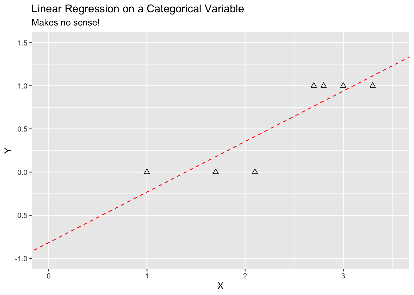
Categorical variables often have no order and if they do, it is not clear the “distance” between levels is the same, e.g., the difference from Low to Medium = the difference from Medium to High.
One cannot calculate, let alone minimize, \(SSE_{Err} = \sum(\hat{y}_i - y_i)^2\) if \(y\) is not a number.
What can we do? Let’s minimize another measure of model error - the error classification rate.
4.2 Error Classification Rate
Instead of measuring a distance like we can do with continuous space, let’s measure a binary response; close does not count. Either the estimate is correct or it is not.
Mathematically, we are interested in the probability of a wrong prediction (or mis-classification), denoted as:
\[ P(\hat{y}_i \neq y_i) \quad \equiv \quad P(\text{predicted response}_i \neq \text{actual response}_i) \tag{4.1}\]
We want to minimize our overall error rate.
This is equivalent to maximizing the correct classification rate (the complement) since
\[
P(\hat{y} \neq y) = 1 - P(\hat{y} = y).
\]
Since we don’t know the true form of \(Y = f(X)\), we don’t know the true probability, so we estimate it.
Let’s define the error classification rate as the number of observations that are mis-classified, divided by the sample size \(n\).
\[ \frac {1}{n} \sum_{i=1}^n I (\hat{Y}_i \neq y_i)\quad \text{ where } \quad I(\hat{Y}_i \neq y_i) = \cases{1 \text{ if } \hat {Y}_i \neq y_i \\ 0 \text{ otherwise}} \tag{4.2}\]
We will use this metric with the KNN Classification Method where “KNN” stands for K Nearest Neighbors.
4.3 KNN Classification
For any given \(X\) and a \(Y\) with \(j\) levels, we will estimate \(P(Y = j) \, \forall\, j\) by using the \(k\) data points “closest” to the given \(X\).
- These \(k\) points are the Nearest Neighbors of \(X\) and we get to choose \(k\), a tuning or hyper-parameter.
- We will define “closest” in terms of the usual Euclidean distance between the two points in \(X_p\) space.
\[ \text{Euclidean Distance}(\vec{X}_1, \vec{X}_2) = \sqrt{\sum_{i = 1}^{p}(X_{2_i} - X_{1_i})^2} \]We then choose the category level \(j\) with the highest (or maximum) estimated probability as the best estimate for \(\hat{Y}\).
\[ \hat{Y}_{x_i,k} = j \text{ where } \frac{1}{n}\sum_{m=1}^{k}I(y_m) \text{ is maximum}\quad \text{with } I(y_m) = \cases{1 \text{ if } y_m =j \\ 0 \text{ otherwise}} \]
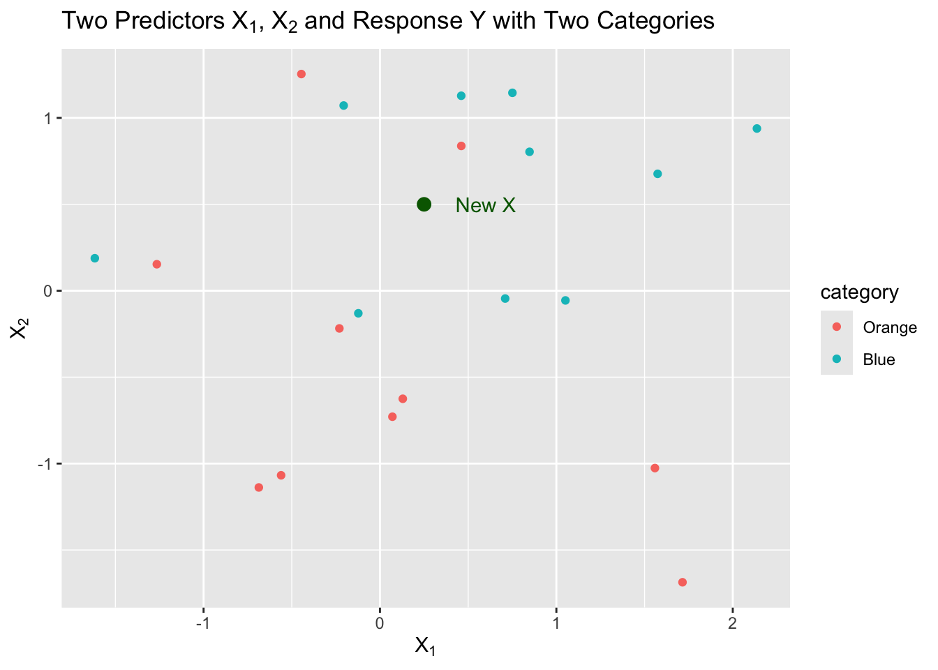
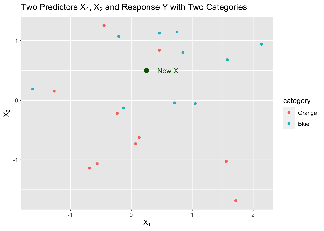
Let’s say we have a sample of 20 observations of two predictors, \(X1\) and \(X2\), with a response \(Y\) that has two categories, “Orange” and “Blue”.
We can visualize this as follows:
Show code
set.seed(123)
x1 <- c(rnorm(10), rnorm(10) + .35)
x2 <- c(rnorm(10), rnorm(10) + .25)
category <- parse_factor(c(rep("Orange", 10), rep("Blue", 10)))
df <- tibble("x1" = x1,
             "x2" = x2,
             "category" = category)

p <- ggplot(df, aes(x1, x2, color = category)) +
  geom_point() +
  labs(title = latex2exp::TeX("Two Predictors $X_1$, $X_2$ and Response Y with Two Categories")) +
  xlab(latex2exp::TeX("$X_1$")) +
  ylab(latex2exp::TeX("$X_2$"))
p
We now want to predict a response for a new point in our two dimensional \(X\) space.
Show code
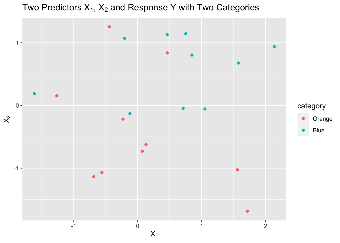
We decide we want to start by using \(k=5\), the five closest neighbors to \(X\). That is the neighborhood.
Show code

We have three neighbors from Blue and two from Orange so we estimate as follows:
\[ \begin{align} \text{3 Blue} & \implies \hat{P}(Y = 2) = \frac{3}{5}\\ \text{2 Orange} & \implies \hat{P}(Y = 1) = \frac{2}{5}\\ \end{align} \] These are estimates of the probability of a correct classification based on the sample proportion.
We want to maximize this probability (which minimizes our error classification rate).
- What is our \(\hat{Y}\) in this example? Which probability is higher?
- In this case, it is Blue, or category 2, since \(\frac{3}{5} > \frac{2}{5}\).
Let’s look at an example.
4.3.1 KNN Example with NFL Field Goal Data
Professor Baron has a data set from ESPN on all of the field goal attempts in the National Football League in 2003.
Read in the data from the following url (http://fs2.american.edu/baron/www/627/R/Field%20goals.txt), while adding in column names for
yards,successandweek.Use
glimpse()andsummmary()to look at the data.
Show code
Rows: 948
Columns: 3
$ yards   <dbl> 30, 41, 50, 22, 33, 44, 40, 55, 49, 51, 27, 39, 26, 38, 36, 50…
$ success <dbl> 1, 1, 1, 1, 1, 1, 1, 0, 1, 1, 1, 1, 1, 1, 1, 1, 1, 1, 1, 0, 0,…
$ week <dbl> 1, 1, 1, 1, 1, 1, 1, 1, 1, 1, 1, 1, 1, 1, 1, 1, 1, 1, 1, 1, 1,… yards success week
Min. :18.0 Min. :0.0000 Min. : 1.000
1st Qu.:28.0 1st Qu.:1.0000 1st Qu.: 5.000
Median :37.0 Median :1.0000 Median : 9.000
Mean :36.5 Mean :0.7975 Mean : 8.989
3rd Qu.:45.0 3rd Qu.:1.0000 3rd Qu.:13.000
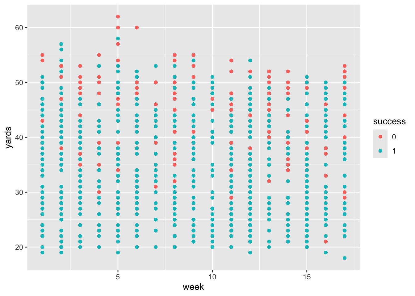
Max. :62.0 Max. :1.0000 Max. :17.000 The data is numeric but it looks like success should be categorical so let’s convert to a factor and check the levels.
Show code
[1] "0" "1" [1] 2 2 2 2 1 2 2 2 2 2 1 2 2 2 2 2 2 1 1 2Since we have two predictors, let’s plot and color code by our categorical response variable.
What is the average success rate across the season?
  0   1
192 756 # A tibble: 2 × 2
f n
<fct> <int>
1 0 192
2 1 756 n
1 0.7974684[1] 0.7974684Can we do better if we include week and yards as predictors? How can we tell if they are “significant” predictors?
This is a standard coaching decision that has many factors but we will try to see if we can do better than the average.
A knn() function is in the {class} package. Install and load the package.
Let’s first just look at overall performance (training data is the entire data set) and predict a kick in week 8 for 55 yards using 10 nearest neighbors - the 10 most similar situations.
Show code
[1] 0
Levels: 0 1
What if we chose a smaller \(k\)?
What if we chose a larger \(k\)?
What would you expect with a \(k\) this large for any week or yardage? Is it helpful?
We could also change the yardage and week.
Show code
[1] 1
Levels: 0 1
What are the implications for using a model like this early in the season say in week 3?
Can we choose a \(k\) so our predictions are better than 0.7974684 accuracy rate?
4.3.2 Training and Testing Split
Let’s split the data into two sets for training and testing.
- Set a seed for the random number generator
- Create a random vector
Zof indexes for rows from the data by sampling without replacement. - Let’s use 50% of the data for training and 50% for testing.
- We can use
Zand-Zto select the training and the testing data so no rows appear in both.
Now let’s recreate our KNN results
- We can test a single data point as before, only now we know the data was not used in training the model.
- We can use predict for entire test data set.
Show code
[1] 1
Levels: 0 1[1] 0
Levels: 0 1Show code
  [1] 1 1 1 1 1 1 1 1 1 1 1 1 1 1 1 1 1 1 1 1 1 1 1 1 1 1 0 1 1 1 1 1 1 1 1 1 1
 [38] 1 1 1 1 1 1 1 1 1 1 1 1 1 0 1 1 1 1 1 1 1 1 1 1 1 1 1 1 1 1 1 1 1 1 1 1 1
 [75] 1 1 1 1 1 1 1 1 1 1 1 1 1 1 1 1 1 1 1 1 1 1 1 1 1 1 1 1 1 1 1 1 1 1 1 1 1
[112] 1 1 1 1 1 1 1 1 1 1 1 1 1 1 1 1 1 1 1 1 1 1 1 1 1 1 0 0 1 1 1 1 1 1 1 1 1
[149] 1 1 1 1 1 1 1 1 1 1 1 1 1 1 1 1 0 1 1 1 1 1 1 0 1 1 1 1 1 1 1 1 1 1 1 1 1
[186] 1 1 1 1 1 1 1 1 1 1 1 1 1 1 1 1 1 1 1 1 1 1 0 1 0 1 1 1 1 1 1 0 1 1 1 1 1
[223] 1 1 1 1 1 1 0 0 1 1 1 1 1 1 1 1 1 0 1 0 0 1 1 1 1 1 1 1 1 1 1 1 1 1 1 1 1
[260] 1 1 0 1 1 1 1 1 1 1 1 0 1 1 1 1 1 1 1 1 1 1 0 1 0 1 1 0 1 1 1 1 1 1 1 1 0
[297] 1 0 1 1 1 1 1 1 1 1 1 1 1 1 1 1 1 1 1 1 1 1 0 1 1 1 1 1 1 1 1 1 1 1 1 1 1
[334] 1 1 1 1 1 1 1 1 1 0 1 1 1 1 1 1 1 1 1 1 1 1 1 1 1 1 0 1 1 1 1 1 1 1 1 0 1
[371] 1 1 1 1 1 1 1 1 1 1 1 0 1 1 1 1 1 1 1 1 1 1 1 1 1 1 1 1 1 1 1 1 1 1 1 1 1
[408] 1 1 1 1 1 1 1 1 1 1 0 1 1 0 1 1 1 1 1 1 1 0 1 1 1 0 1 0 1 1 0 1 1 1 1 1 1
[445] 1 1 1 1 0 1 1 1 1 1 1 0 1 1 1 1 1 1 1 1 1 1 1 1 1 1 1 1 1 1
Levels: 0 1[1] 4744.3.3 Example by Hand
We want to predict if a new drug will have serious side effects based on two quantitative predictors.
We have the following data for 5 randomly chosen test subjects.
| Subjects | S1 | S2 | S3 | S4 | S5 |
|---|---|---|---|---|---|
| \(x_1\) | 0 | 0 | 1 | 1 | 0 |
| \(x_2\) | 2 | 3 | 3 | 4 | 4 |
| Side Effects (YesNo) | N | Y | Y | N | N |
- Subjects are broken into two sets: train(1, 3, 4) and test (2,5)
- Create test set predictions for two models with \(k=1\) and \(k=3\).
- Calculate the Misclassification rate for each model.
| Test | \(x_1\) | \(x_2\) | \(Y\) | Dist to S2(0,3) | Dist to S5 (0,4) | \(k=1\) | \(k=1\) | \(k= 3\) | \(k = 3\) |
|---|---|---|---|---|---|---|---|---|---|
| S2 Neigh | S5 Neigh | S2 Neigh | S5 Neigh | ||||||
| S1 | 0 | 2 | N | \(1=\sqrt{0^2 + 1^2}\) | \(2=\sqrt{0^2 + 2^2}\) | 1/2 | 1 | 1 | |
| S3 | 1 | 3 | Y | \(1=\sqrt{1^2 + 0^2}\) | \(\sqrt{2}=\sqrt{1^2 + 1^2}\) | 1/2 | 1 | 1 | |
| S4 | 1 | 4 | N | \(\sqrt{2}=\sqrt{1^2 + 1^2}\) | \(1=\sqrt{1^2 + 0^2}\) | 1 | 1 | 1 |
| Test | \(x_1\) | \(x_2\) | \(Y\) | Dist to S2(0,3) | Dist to S5 (0,4) | \(k=1\) | \(k=1\) | \(k= 3\) | \(k = 3\) |
|---|---|---|---|---|---|---|---|---|---|
| S2 Neigh | S5 Neigh | S2 Neigh | S5 Neigh | ||||||
| S1 | 0 | 2 | N | \(1\) | \(2\) | 1 /2 | 1 | 1 | |
| S3 | 1 | 3 | Y | \(1\) | \(\sqrt{2}\) | 1/2 | 1 | 1 | |
| S4 | 1 | 4 | N | \(\sqrt{2}\) | \(1\) | 1 | 1 | 1 |
| \(\hat{y}\) | 1/2 Y 1/2 N | N | N | N | |||||
| \(y\) | Y | N | Y | N | |||||
| Mis-Class | 1/2 | 0 | 1 | 0 | |||||
| Rate | .5/2= .25 | 1/2=.5 |
There is no single method for breaking ties in either the nearest neighbor or the majority rules. Options include:
- Randomly chose one candidate from the set of ties,
- Choose them all.
- Increase \(k\) until the tie is broken for that point.
The class::knn() function includes all the candidates and then breaks ties at random in the majority rules.
This is usually not a major issue for large data sets for either prediction or calculation of performance metrics.
So in general, how do we evaluate performance, and tune our model? Which \(k\) is better?
4.4 Flexible or Restrictive
Recall optimizing the bias-variance trade off requires finding the right level of flexibility or restrictiveness in the model.
As you think about KNN, how does the model flexibility change with \(k\)?
- Model tries to follow the sample data more closely.
- With \(k = 1\), \(\hat{Y}\) is based on a single value from the sample.
- Lower \(k\) is more flexible.
- Higher \(k\) uses more and more data points so if \(k = n\) it is estimating the sample mean.
- Higher \(k\) is more restrictive.
- This is opposite of linear regression where more parameters is more flexible.
4.5 Evaluating Classification Model Performance
To tune a KNN classification model ( to find the “best” \(k\)), we have to be able to quantitatively evaluate the model performance on the testing data and compare to other models that may be more restrictive (higher \(k\)) or more flexible (lower \(k\)).
We have \(X_1, \ldots, X_p\) predictor variables and \(Y\) is our categorical response variable.
We are estimating the true form of \(Y=f(X)\) by estimating \(\hat{Y}\) as a categorical response.
Using the complement form of Equation 4.1, we get a form of Equation 4.2 such that
\[ \text{Classification Rate}\,= \frac {1}{n} \sum_{i=1}^n I (\hat{Y}_i = y_i)\quad \text{ where } \quad I(\hat{Y}_i = y_i) = \cases{1 \text{ if } \hat {Y}_i = y_i \\ 0 \text{ otherwise}} \]
This is interpreted as the number of times we predicted correctly divided by the total sample size, or, the sample proportion of correct predictions.
- The error classification rate is the complement of the classification rate. It is the proportion of incorrect predictions.
- We can calculate either of these metrics on the training data (from 1 to 100% of the data) or on the test data used for prediction.
We can use this metric to tune the model by choosing the best \(k\); the \(k\) that minimizes the Testing (aka Prediction) Error Rate.
If the \(k\) is too little (too flexible), the estimate \(\hat{y}\) may not be reliable. It is based on small sets of data which leads to overfitting with High Variance for \(\hat{y}\).
If the \(k\) is too large (too restrictive), the estimate \(\hat{y}\) is based on irrelevant, remote points which leads to underfitting with high Bias for \(\hat{y}\).
4.6 Binary Classification Confusion Matrices
4.6.1 Types of Classification Methods
We will consider two types of classification methods.
- Some classification methods make direct predictions of the outcome, e.g., true or false. KNN is one of those.
- Other classification methods estimate the probability or likelihood of an event being true or false based on the “strength of the signal”. Logistics Regression is an example.
- This strength of signal (versus noise), could be an estimated probability or the ratio of dark pixels in an area to light pixels in the area.
- Methods that estimate the strength of the signal have to set or choose a threshold to convert the estimated strength to a final prediction.
- As an example, if the strength (or probability) is greater than some value, predict TRUE, otherwise FALSE.
By ensuring each classification method results in a prediction, we can examine the prediction performance using a Confusion Matrix.
- Confusion Matrices organize the counts of various outcomes in a table so one can calculate error rates or other metrics to assess performance and tune the model (aka the classifier).
When we have binary response data (positives and negatives) we can calculate two metrics based solely on the number of samples or observations, \(n\), the number of positives, \(P\), and the number of negatives, \(N\).
- Actual Positive Rate: \(P/n\) - the average number of positives in the sample.
- Actual Negative Rate: \(N/n\) - the average number of negatives in the sample.
4.6.2 Binary Classification Outcomes
When we create a model with \(p\) predictors \(X\), for a binary classification problem, (True/False, Yes/No, Positive/Negative, …), there are four possible outcomes for predictions.
We will define the following metrics in terms of TRUE and FALSE but the same definitions apply for YES/NO or SUCCESS/FAILURE etc..
True Positive: a predicted value of \(\hat{y}_i= \text{TRUE}\) is correct as the actual value is \(y_i = \text{TRUE}\) or \(\hat{y}_i = y_i= \text{TRUE}\).
-
False Positive: a predicted value of \(\hat{y}_i= \text{TRUE}\) is incorrect as the actual value is \(y_i = \text{FALSE}\) or \(\hat{y}_i \neq y_i\).
- Also known as Type I error
-
False Negative: a predicted value of \(\hat{y}_i= \text{FALSE}\) is incorrect as the actual value is \(y_i = \text{TRUE}\) or \(\hat{y}_i \neq y_i\).
- Also known as Type II error
True Negative: a predicted value of \(\hat{y}_i= \text{FALSE}\) is correct as the actual value is \(y_i = \text{FALSE}\) or \(\hat{y}_i = y_i= \text{FALSE}\).
4.6.3 2x2 Confusion Matrices
A 2x2 confusion matrix shows the performance of a model on a sample of size \(n\) by organizing the \(n\) predictions into each of the four possible outcomes and showing the counts for each outcome.
- A confusion matrix allows one to see how much or how little a model “confuses” the two classifications.
| Actual \ Predicted | Positive (PP) | Negative (PN) |
|---|---|---|
| Positive (P) | True Positive (TP) count | False Negative (FN) count |
| Negative (N) | False Positive (FP) count | True Negative (TN) count |
Columns and Rows add up to their top/left totals
- \(\text{PP} + \text{PN} = n\)
- \(\text{TP} + \text{FN} = P\)
- \(\text{FP} + \text{TN} = N\)
- \(\text{TP} + \text{FP} = PP\), \(\text{FN} + \text{TN} = PN\)
- \(\text{TP} + \text{FN} + \text{FP} + \text{TN} = n\)
4.6.4 Confusion Matrix Performance Metrics
Given the counts, we can then define corresponding rates for each of the four outcomes as:
-
True Positive Rate: \(TPR = TP/P\): ratio of True Positive Predictions to actual Positives.
- Other names: Sensitivity, Hit Rate, Probability of Detection something that is actually there, or Power.
- \(P(\hat{Y}) = 1\, |\, Y = 1)\) as a Conditional Probability.
-
False Positive Rate: \(FPR = FP/N\): ratio of False Positive Predictions to actual Negatives.
- Other names: False Alarm rate, Overestimation Rate
- \(P(\hat{Y}) = 1\, |\, Y = 0)\)
-
False Negative Rate: \(FNR = FN/P\): ratio of False Negative Predictions to actual Positives.
- Other names: Miss rate
- \(P(\hat{Y}) = 0\, |\, Y = 1)\)
-
True Negative Rate: \(TNR = TN/N\): ratio of True Negative Predictions to actual Negatives.
- Other names: Specificity
- \(P(\hat{Y}) = 0\, |\, Y = 0)\)
Each of these rates can be used as a performance metric for tuning to optimize the model performance based on question being asked and the purpose of the model.
-
Other metrics are also defined and used for tuning or optimizing the model.
- Accuracy: \((TP + TN)/n\): ratio of correct predictions to total predictions or average correct classification rate.
- Here are some examples from a Wikipedia discussion on confusion matrices in machine learning, Binary Classification Confusion Matrix Metrics
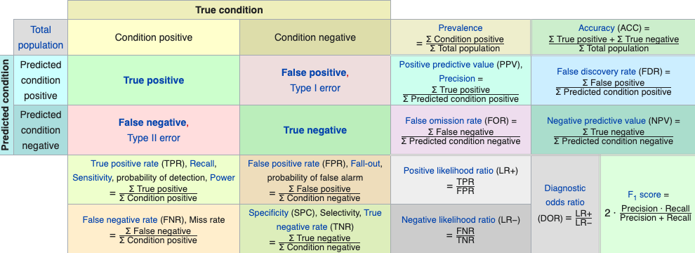
- We can use multiple metrics in a Receiver Operating Characteristic (ROC) curve to help balance the bias and variance in a model or and choose between models.
4.7 The Receiver Operating Characteristic Curve
The Receiver Operating Characteristic curve or ROC curve is a graphical method for describing the performance of a “receiver” based on two performance characteristics and a range of thresholds.
- ROC Curves have been used since World War II when they were originally developed to help compare different radar systems ability to differentiate between signal (Success) and noise (Failure).
- The receiver refers to the system under study.
- The characteristics are usually a desirable performance characteristic and an undesirable performance characteristic where the two characteristics are linked such that increasing one can also increase the other so there is a trade off to be made.
ROC curves are useful in binary classification methods where a threshold is used to determine if an event is a success or failure based on the strength of signal (hit or miss, signal or noise, cancer or non-cancer, … .
- ROC curves are used in many different fields for a variety of binary classification problems to compare models.
- Standard ROC curves use as characteristics the True Positive Rate and the False Positive Rate of the receiver when it is operating under fixed conditions (here, our \(k\)).
The ROC is a plot of desirable True Positive Rate (TPR), for a given threshold, on the \(Y\) axis, against the undesirable False Positive Rate (FPR) for that same threshold on the \(X\) axis.
- The TPR and FPR are calculated for many different threshold values to create the ROC curve.
- The TPR can be considered the “Benefit” while the FPR can be considered the “Cost” of the model outcomes for that threshold.
- We want the TPR to be high and the FPR to be low but there is a trade off.
- An abline with slope 1 indicates when \(TPR = FPR\) or equal performance between good and bad.
The Area Under the Curve (AUC) is the total benefit of a model across the range of thresholds.
We would like an ROC curve to look something like the following:
- We want a sharply rising curve on the left so a high TPR at a low FPR.
- The greater the AUC, the better the performance of the model. This is often used when comparing multiple models, each with their own ROC curve.
Show code
df <- tibble(x = seq(1:100)/100, y = c(9.2*x[1:10],  (rep(.92, 90) + (seq(1:90)/4000))))
ggplot(df, aes(x, y)) +
  geom_line() +
  ylim(0, 1) +
  xlim(0, 1) +
  xlab("False Positive Rate") +
  ylab("True Positive Rate") +
  geom_line(data = tibble(x = c(0,1), y = c(0,1)), aes(x, y), color = "red",
            lty = 3) +
  # geom_line(data = tibble(x = c(.05,.15), y = c(.85,1)), aes(x, y),
  #           color = "darkgreen", lty = 1, linewidth = 2) +
  # annotate("text", x = .15, y = .95, label = "Elbow in the Curve", color = "darkgreen",
  #          hjust = 0) +
  geom_area(data = tibble(x = c(0, .1, 1), y = c(0, .92, max(df$y))),
            aes(x = x, y = y), fill = "blue", alpha = .25) +
  annotate("text", x = .5, y = .7, label = "AUC - Area under the Curve", color = "blue")
- Normally curves are not as straight or as nice.
We can use the ROC curve to look for the “best” threshold based on an “elbow” or ’knee” in the curve.
This is the threshold where the later increase in TPR is minimal (the benefit) compared to the later increase in FPR (the cost).
- Choose \(k\) to match the elbow in the curve.
Show code
ggplot(df, aes(x, y)) +
  geom_line() +
  ylim(0, 1) +
  xlim(0, 1) +
  xlab("False Positive Rate") +
  ylab("True Positive Rate") +
  geom_line(data = tibble(x = c(0,1), y = c(0,1)), aes(x, y), color = "red",
            lty = 3) +
  geom_line(data = tibble(x = c(.05,.15), y = c(.85,1)), aes(x, y),
            color = "darkgreen", lty = 1, linewidth = 2) +
  annotate("text", x = .15, y = .95, label = "Elbow in the Curve", color = "darkgreen",
           hjust = 0) #+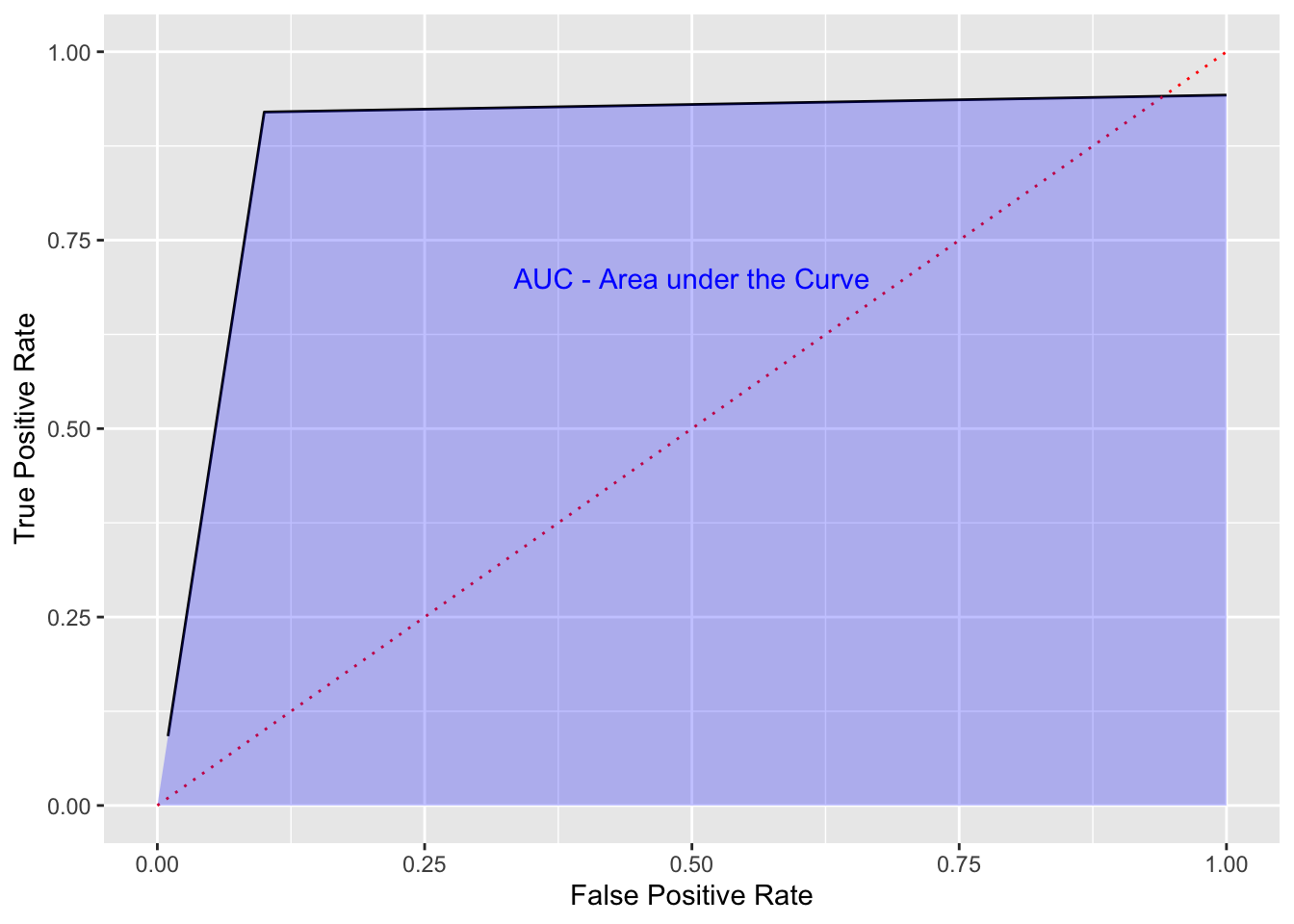
4.7.1 Finding a Good \(k\) Using ROC Curves
Now in this case, \(k\) is not really a threshold. In fact we are comparing different KNN models, not one model across different thresholds.
- That means the ROC curve may not be a “relatively smooth” monotonic curve, but it could be useful.
Our Steps
- Pick a \(k.\)
- Identify the neighborhood.
- Predict \(\hat{y}_i\) for each point in the test data and count the number of each of the four outcomes by comparing \(\hat{y}_i\) to \(y_i.\)
- Calculate the True Positive Rate and the False Positive Rate for that \(k.\)
- Repeat for each \(k\) of interest.
- Plot the Error Classification Rate for each \(k\) and then the ROC Curve.
Let’s use a for-loop to calculate TPR and FPR for \(k\) from 1 to 100 on the Field Goal data.
Then, select a good \(k\) based on the error classification rate.
[1] 948Z = sample(nrow(fg), training_pct*nrow(fg))
# Set our test and training data
Xtrain = fg[Z,c("yards", "week")] # Our training set X
Ytrain = fg$success[Z] # Our training set y
Xtest = fg[-Z,c("yards", "week")] # The test data set
Ytest = fg$success[-Z]
# Initialize data
err_class <- rep(1:100)
tpr <- rep(1:100)
fpr <- rep(1:100)
# run the loop
for (k in 1:100) {
Yhat <- knn(Xtrain, Xtest, Ytrain, k = k)
err_class[k] <- mean(Yhat != Ytest) # The prediction is not correct
tpr[k] <- sum(Yhat == 1 & Ytest == 1) / sum(Ytest == 1) # TP/P
fpr[k] <- sum(Yhat == 1 & Ytest == 0) / sum(Ytest == 0) # FP/N
}
ggplot(tibble(err_class, k = 1:100), aes(x = k, y = err_class)) +
geom_line()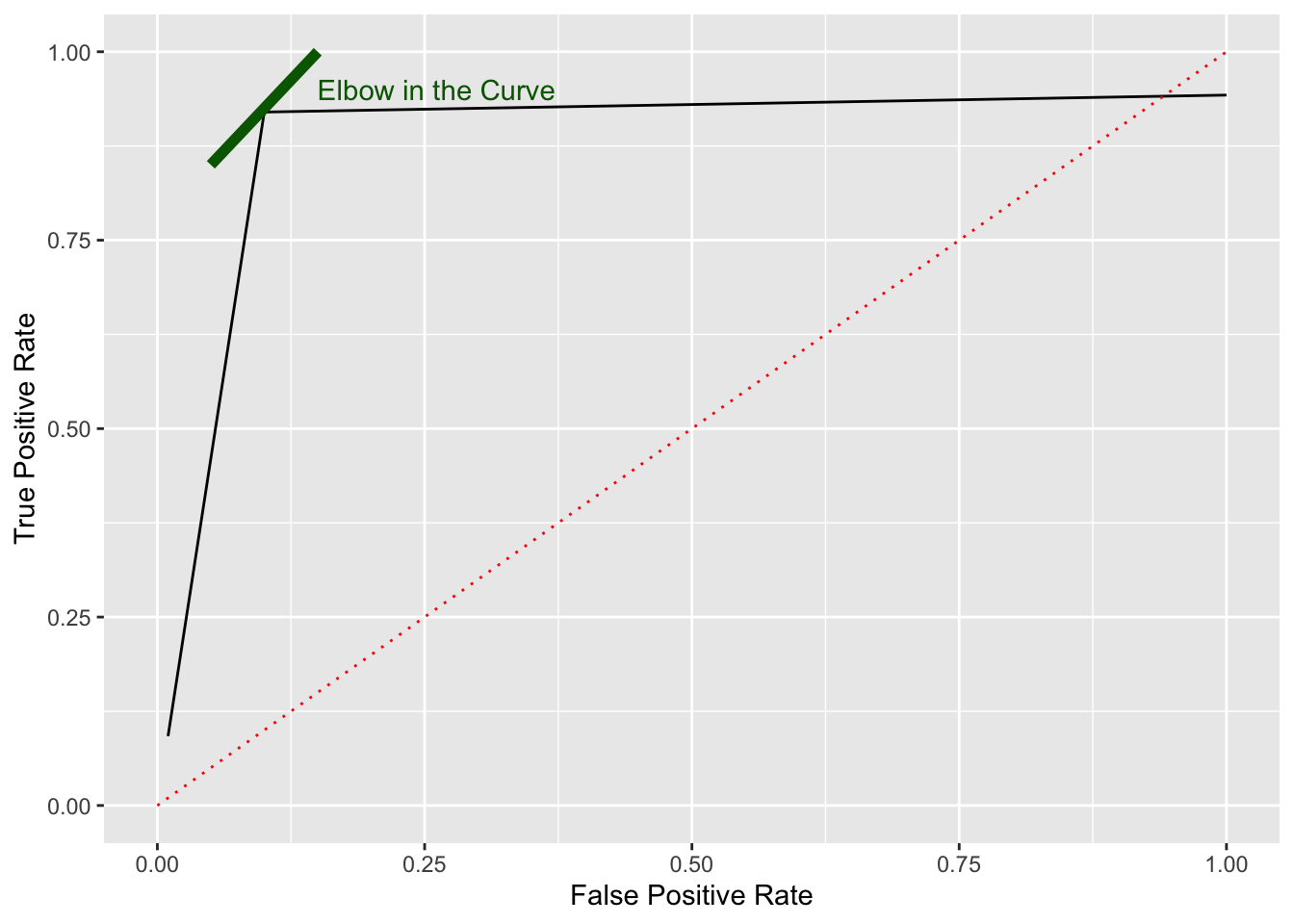
[1] 19[1] 0.185654[1] 0.814346# calculate the accuracy for the best k
Yhat <- knn(Xtrain, Xtest, Ytrain, k = which.min(err_class))
table(Ytest, Yhat) # the Confusion Matrix Yhat
Ytest 0 1
0 21 75
1 16 362[1] 0.8080169- Note the variability if we change seed or size of the training set.
Use the table() function with \(Y_i^{test}\) and \(\hat{Y}_i\) to get a confusion matrix for the predicted outcomes.
     Yhat
Ytest   0   1
    0   0  96
1 0 378[1] 0.7974684With \(k=100\), our neighborhood is so large we always predict Success.
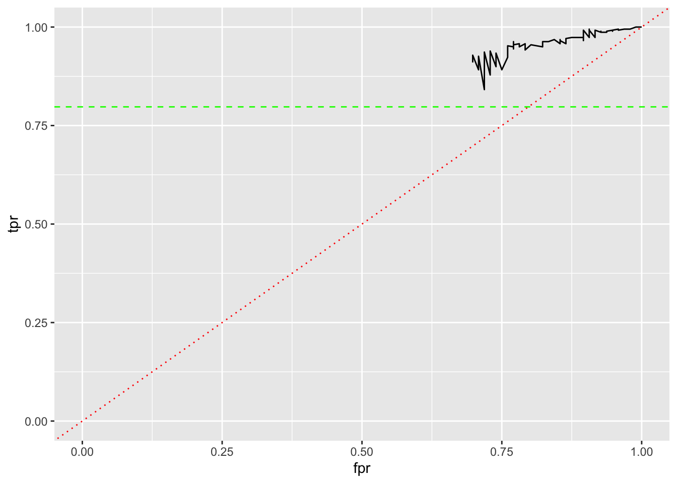
Let’s look at an ROC curve and see if it helps identify a “best” K based on FPR and TPR.
- Can we see an elbow in the black line?
- What do the red and green lines represent on this graph?
- How do we interpret the black line?
Show code
     Yhat
Ytest   0   1
    0  22  74
    1  16 362
Show code
If we believe the point with the lowest FPR and then the highest TPR is the best, we can find the \(k\) for it.
# A tibble: 1 × 3
      k   fpr   tpr
  <int> <dbl> <dbl>
1    12 0.698 0.929
If we believe the point with the highest TPR and then the lowest FPR is the best, we can find the \(k\) for it.
# A tibble: 17 × 3
       k   fpr   tpr
   <int> <dbl> <dbl>
 1    84 0.990     1
 2    85 1         1
 3    86 1         1
 4    87 1         1
 5    88 1         1
 6    89 1         1
 7    90 1         1
 8    91 1         1
 9    92 1         1
10    93 1         1
11    94 1         1
12    95 1         1
13    96 1         1
14    97 1         1
15    98 1         1
16    99 1         1
17   100 1         1
Plotting those points with a LOESS smoother shows a range of options with no clear “best”.
Show code
     Yhat
Ytest   0   1
    0  22  74
    1  15 363
Show code
ggplot(tibble(tpr, fpr), aes(x = fpr, y = tpr)) +
  geom_line() +
  geom_abline(color = "red", lty = 3) +
  ylim(0.65, 1) + xlim(0.65, 1) +
  geom_hline(yintercept = mean(as.numeric(fg$success)-1), color = "green", lty = 2) +
  geom_point(data = filter(tibble(k = seq_along(fpr), tpr, fpr), k == 12),
             size = 3, color = "blue") +
  geom_point(data = filter(tibble(k = seq_along(fpr), tpr, fpr), k == 84),
             size = 3, color = "purple") +
  geom_smooth(se = FALSE)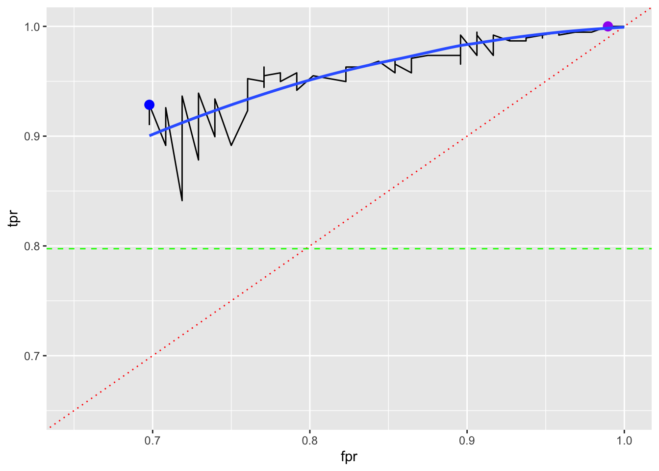
4.7.2 Let’s Try with a Reduced Model with Just yards.
-
knn()requires at least two variables so we can add a dummy variable of 1.
Show code
fg1 <- tibble(dummy = rep(1, nrow(fg)), yards =  fg$yards)
err_class2 <- tpr2 <- fpr2 <- rep(1:100)
Xtrain <- fg1[Z,]
Xtest <- fg1[-Z,]
for (k in 1:100) {
  Yhat <- knn(Xtrain, Xtest, Ytrain, k = k)
  err_class2[k] <- mean(Yhat != Ytest) # The prediction is not correct
  tpr2[k] <- sum(Yhat == 1 & Ytest == 1) / sum(Ytest == 1) # TP/P
  fpr2[k] <- sum(Yhat == 1 & Ytest == 0) / sum(Ytest == 0) # FP/N
}

ggplot(tibble(err_class2, k = 1:100), aes(x = k, y = err_class2)) +
  geom_line(color = "blue") +
  geom_line(data = tibble(err_class, k = 1:100), mapping = aes(x = k, y = err_class))
[1] 0.814346[1] 0.8101266ROC Curve
Show code
ggplot(tibble(tpr, fpr), aes(x = fpr, y = tpr)) +
  geom_line() +
  geom_abline(color = "red", lty = 3) +
  ylim(0.65, 1) + xlim(0.65, 1) +
  geom_hline(yintercept = mean(as.numeric(fg$success)-1), color = "green", lty = 2) +
  geom_line(data = tibble(tpr2, fpr2), mapping = aes(x = fpr2, y = tpr2),
color = "blue") 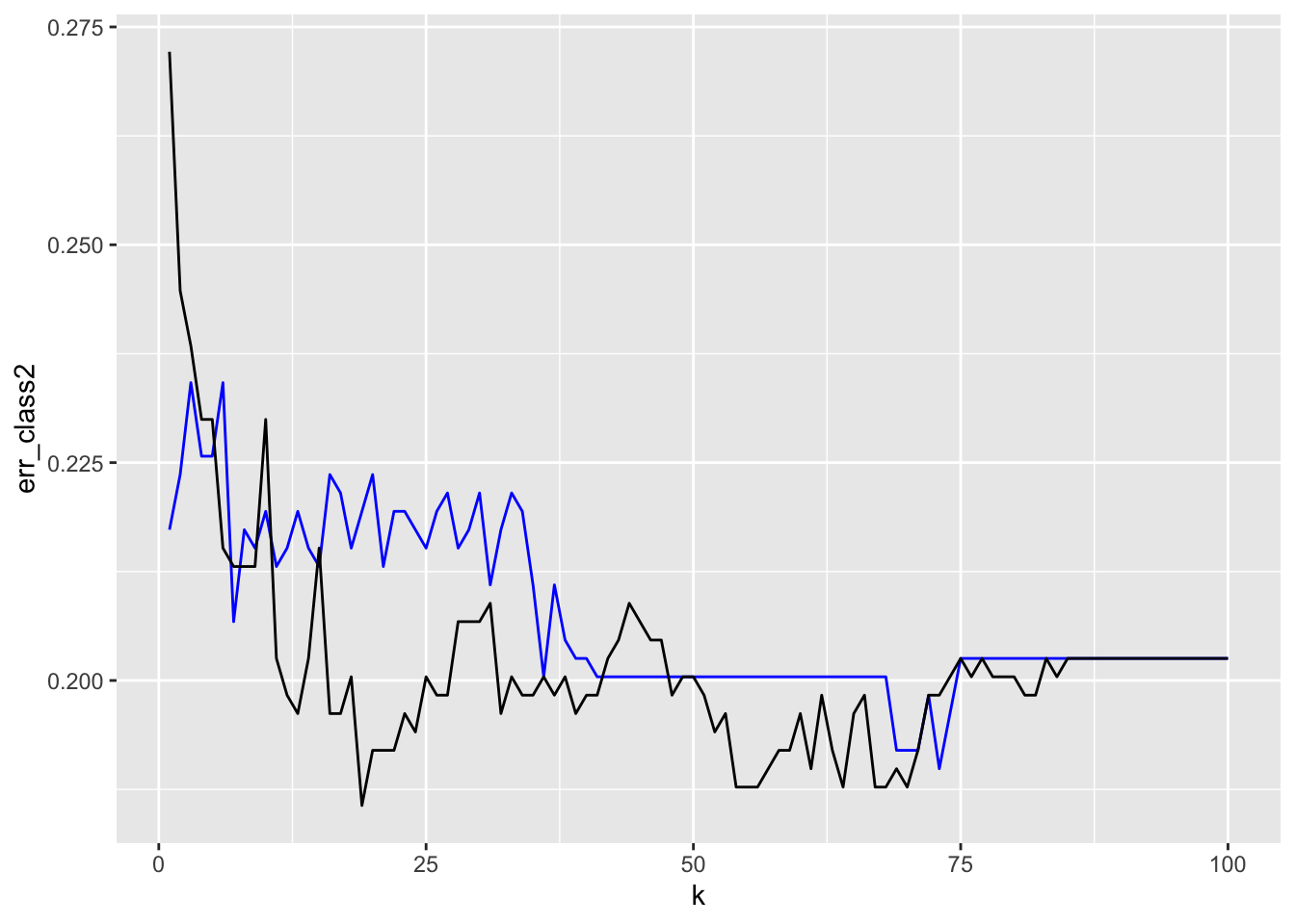
The points are Not in the order of the \(k\).
How would you interpret this plot in comparing the two models?
Different models but the results are close although the Full model gives access to lower FPR.
4.7.3 Summary of KNN
A non-parametric classification method useful for predicting a categorical outcome based on multiple predictors.
4.7.4 Foreshadowing Logistic Regression
- In contrast to KNN, Logistic Regression is a parametric method for classification we will discuss next.
Show code
       1
2.055085
Use the argument type = "response" to get the prediction in the \(Y\) space or as a probability.
        1
0.9260122 1
0.8572845 Note we can use summary here as well to check the “significance” of the predictors.
Call:
glm(formula = success ~ yards + week, family = "binomial", data = fg)

Coefficients:
            Estimate Std. Error z value Pr(>|z|)
(Intercept)  6.29969    0.51105  12.327   <2e-16 ***
yards       -0.11274    0.01076 -10.477   <2e-16 ***
week        -0.05243    0.01832  -2.862   0.0042 **
---
Signif. codes:  0 '***' 0.001 '**' 0.01 '*' 0.05 '.' 0.1 ' ' 1

(Dispersion parameter for binomial family taken to be 1)

    Null deviance: 955.38  on 947  degrees of freedom
Residual deviance: 808.86  on 945  degrees of freedom
AIC: 814.86

Number of Fisher Scoring iterations: 5
Now let’s look at Logistic Regression in more detail.
4.8 Logistic Regression (Chap 4.3)
4.8.1 Logistics Regression is Useful for a Binary Response
Logistic Regression is a classification method for categorical response data.
- When we had a categorical predictor, we used \(k-1\) dummy variables of 0 and 1 for \(k\) category levels.
For a categorical response variable, OLS will not work for \(k>2\).
We could use dummy variables and fit \(k-1\) logistics regression equations but this can be onerous.
- This is why logistics regression is mostly used for \(k =2\), binary classification, and other methods are more popular for \(k>2\).
- KNN, or Linear or Quadratic Discriminant analysis as well as decision trees or Support Vector Machines (SVM) are more popular for \(k>2\).
- With \(k=2\) we need just one dummy variable.
We could fit a linear regression using OLS for \(k=2\), so \(Y = 0 \text{ or } 1\).
- OLS will calculate residuals and sum the squared differences.
- However, as we saw in Figure 4.1, the OLS prediction can be unbounded and values of \(\hat{y} <0\) or \(\hat{y} >1\) do not make sense.
In the binary case of logistic regression, we are not trying to predict the category level directly, e.g., 0 or 1, but predict the probability or likelihood of a Success, a 1.
- A Bernoulli trial is situation with a binary outcome \(Y\) for each trial. The value of the outcome (1 or 0) is a random variable where it has the value 1 (a success) with probability \(p\).
- These random variables are described by a Bernoulli Distribution where the \(E[Y] = P(Y=1) = p\).
- The Bernoulli distribution is a subfamily of the Binomial Distribution.
- The Binomial Distribution describes the number of successes in \(n\) independent Bernoulli trials where each success has probability \(p\).
In Logistic Regression with \(k=2\), the response is a Bernoulli random variable with parameter \(p\) as the probability of success, which is the same as Binomial\((n=1, p)\).
For \(0<\hat{y} <1\), if we we think of \(Y\) as having a Bernoulli distribution, it can be shown that \(\hat{y}\) is the expected value of \(Y\) or \(E[Y] = P(y =1)\).
4.8.2 Estimating Probabilities with the Logistic Function
We want to use Logistic Regression to estimate the probability of a success.
Let \(p(X)\) be a function denoting the conditional probability of a success \(Y=1\) given the values of a predictor \(X\), or
\[ p(X) = P(Y=1|X) \]
If we try to fit \(P(X) = \beta_0 + \beta_1 X\) we get the unbounded results in Figure 4.1 (where the \(Y\) axis represents a probability).
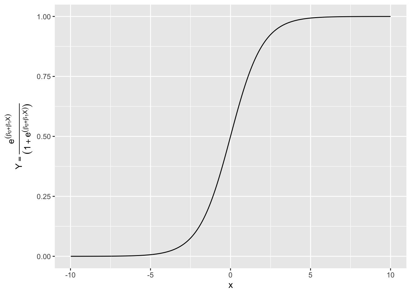
To estimate probabilities, we need a function that is bounded between 0 and 1. While many functions could do this, in Logistic Regression we use the Logistic Function.
- The Logistic Function (aka a Logistic Curve or an S-curve) has the following formula.
\[ p(X) = \frac{e^{\beta_0 + \beta_1X}}{1 + e^{\beta_0 + \beta_1X}} \tag{4.3}\]
- This function is always positive and the difference between the top and bottom of the ratio is 1 so \(0<p(X)<1\).
With a little algebra Equation 4.3 gives us
\[ \frac{p(X)}{1-p(X)} = e^{\beta_0 + \beta_1X} \tag{4.4}\]
Equation 4.4 is known as the Odds or Odds Ratio as it is the ratio of the odds (the probabilities).
- Note it can range from \(0 \rightarrow \infty\).
If we take the log() of both sides of Equation 4.4, we get
\[ \ln{\frac{p(X)}{1-p(X)}} = \beta_0 + \beta_1X \tag{4.5}\]
- The left side of Equation 4.5 is known as the logit or log(odds).
- This can range from \(-\infty\) to \(\infty\).
- Note that the right side of Equation 4.5 is linear in \(X\) as we saw in OLS.
- Here, increasing \(X\) by one unit changes the log odds by \(\beta_1\).
- This means the amount that \(p(X)\) changes due to a one-unit change in \(X\) depends on the current value of \(X\).
If we solve the logistic regression using Equation 4.5, we can do the reverse algebra to get \(p(Y=1\)) as
\[ \begin{align} \ln{\frac{p(X)}{1-p(X)}} &= \beta_0 + \beta_1X &\implies \\ \frac{p(X)}{1-p(X)} &= e^{\beta_0 + \beta_1X} &\implies \\ p(X) &= (1-p(X))e^{\beta_0 + \beta_1X} &\implies \\ p(X) &= e^{\beta_0 + \beta_1X} - p(X)e^{\beta_0 + \beta_1X} &\implies \\ p(X) + p(X)e^{\beta_0 + \beta_1X} &= e^{\beta_0 + \beta_1X} &\implies \\ p(X)(1 + e^{\beta_0 + \beta_1X}) &= e^{\beta_0 + \beta_1X} &\implies \\ p(X) &= \frac{e^{\beta_0 + \beta_1X}} {(1 + e^{\beta_0 + \beta_1X})} \end{align} \] which matches Equation 4.3.
4.8.3 Examples of Logistic Function Curves
Show code
What happens if we change the intercept to \(\beta_0 = 2\)
Show code
Note the shift to the right. The \(\beta_0\) represents the logit of the probability when \(x=0\).
What happens if we change the slope to \(\beta_1 = 2.\)
Show code
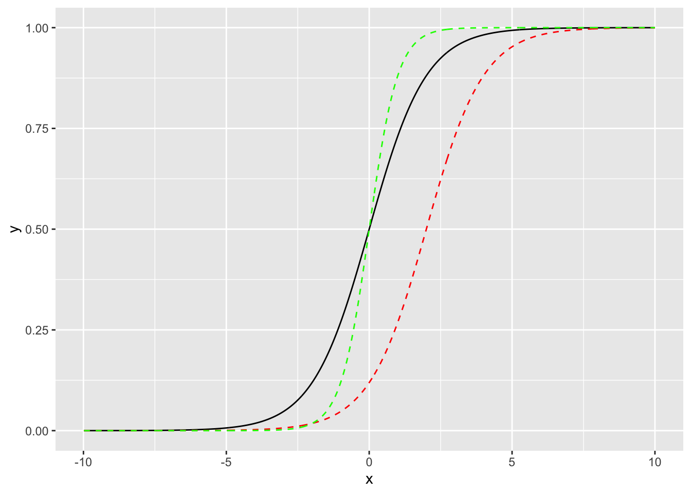
To explore the effect of changes in the \(\beta_j\) on the shape of the logistic curve, try the app at Explore the Logistic Curve.
4.8.4 Why the Logit Function?
We can see the logistic curves have some nice properties.
- Our curve gives reasonable predictions when we are close to 0 and 1.
- When \(Y\) is close to 0, there is very little change in the curve.
- When \(Y\) is close to 1, there is very little change in the curve.
We can describe this mathematically (using some calculus terms) where the derivative of \(Y\) with respect to \(X\) (or the change in \(Y\) as \(X\) changes by a small amount) has the following relationship (\(k\) is a proportionality constant for scale).
\[ \frac{dY}{dX} =k * Y (1-Y) \]
This relationship means whenever \(Y\) is close to 0 or 1, the change in \(Y\) is small for small changes in \(X\).
One can use methods from calculus to figure out what function \(Y\) has this derivative.
- We can solve this differential equation for \(Y\), which is \(p(X)\), so we know \(0<Y<1\).
- Let’s separate the variables and integrate each side and then manipulate with algebra to get
\[ \begin{align} \int \frac{dY}{Y(1 - Y)} &= \int k dX \\ \int\left(\frac{1}{Y} + \frac{1}{1-Y}\right)dY &=kX + c \\ \int\frac{dY}{Y} + \int\frac{dY}{1-Y} &=kX + c \\ \ln(Y) - \ln(1-Y) &=kX + c \quad \text{we can drop the |Y| as we know Y is in [0,1]}\\ \ln\left(\frac{Y}{1-Y}\right) &= kX + c \quad \text{this is the logit or log odds of the probability Y}\\ &\text{Let's solve for Y} \\ \frac{Y}{1-Y} &= e^{kX + c} \\ Y &= e^{kX + c} - Ye^{kX + c} \\ Y (1 + e^{kX + c}) &= e^{kX + c} \\ Y &= \frac{e^{kX + c}} {(1 + e^{kX + c})} \end{align} \]
- Rearrange the exponent term and use \(\beta_0\) for \(c\) and \(\beta_1\) for \(k\) and we have Equation 4.3.
Taking the log of Equation 4.3 now makes the logit a linear function of the \(X_i\) as in Equation 4.5, so we can estimate our parameters.
4.8.5 Multiple Logistic Regression
Equation 4.3 can be generalized for multiple predictors as
\[ p(X) = \frac{e^{\beta_0 + \beta_1X + \ldots, \beta_pX_p}}{1 + e^{\beta_0 + \beta_1X + \ldots, \beta_pX_p}} \tag{4.6}\]
To interpret the coefficients
- \(\beta_0\): We estimate \(\widehat{E[Y]} = \hat{p} = \frac{e^{\beta_0}}{1+e^{\beta_0}}\) when all \(X_i = 0\) or
\[ \hat{\beta}_0 = \ln\frac{\hat{p}}{1-\hat{p}} \quad \text{the logit of }\hat{p} \text{ when all }X_i = 0 \]
- \(\beta_i\): The larger the value of an individual \(\beta_i\) the greater the effect of the \(X_i\) on the expected response, either positive or negative, all other variables held the same.
4.8.6 Estimating \(\hat{p}\) Using Maximum Likelihood
We could try to use OLS to minimize the Mean Squared Error for the residuals from the logistic curve.
Consider Figure 4.2 with some sample points on it. This shows the probability space for \(Y\) for our data.
Show code
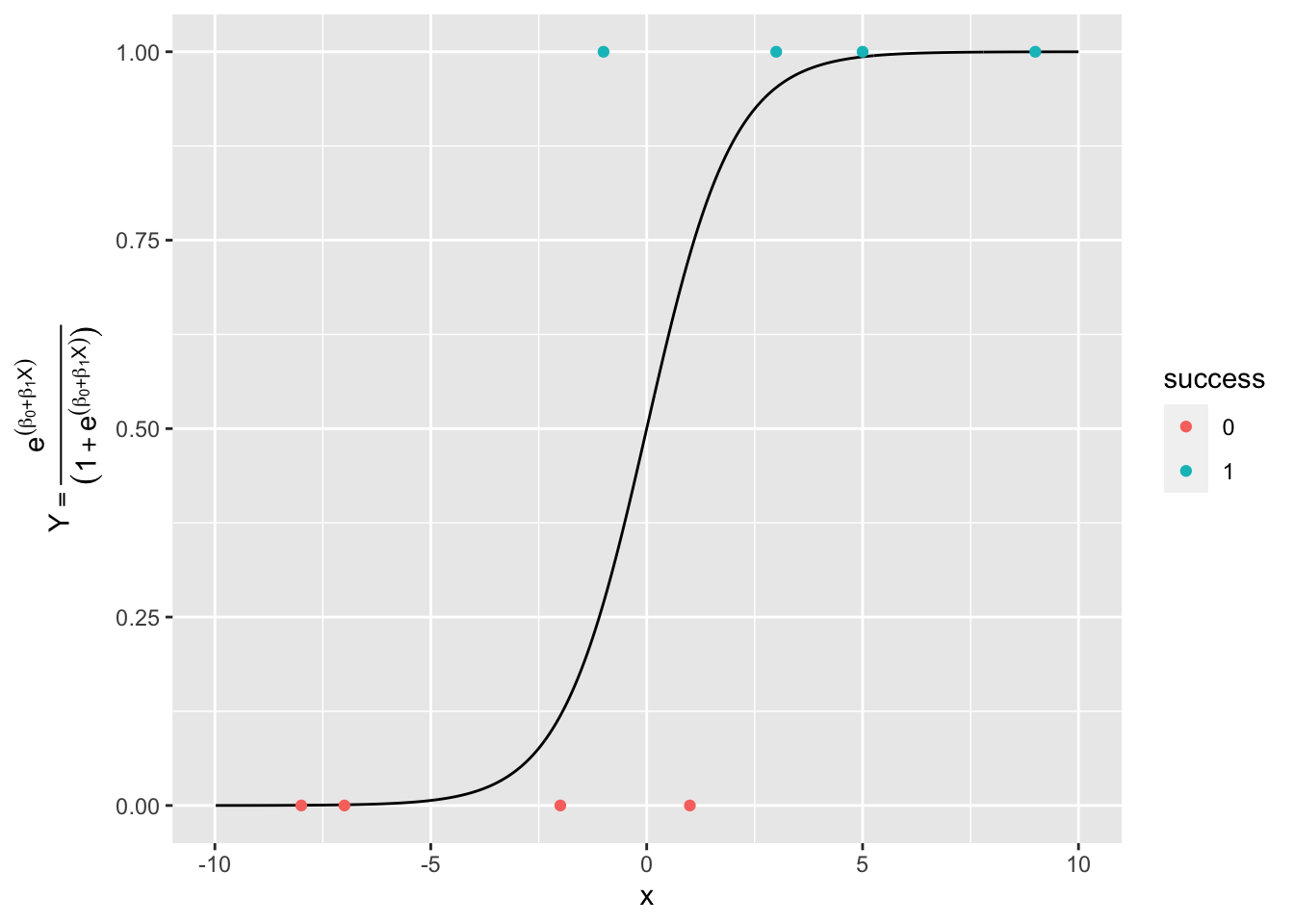
Let’s apply the logit transform to our data to get to the log-odds or logit view of \(Y\).
- What is the value of \(\ln(1/(1-1)\) or \(\ln(0/(1-0)\)?
Show code
df_example$logit_y <- log(df_example$y/(1-df_example$y))
df$logit_line <- log(df$y/(1-df$y))

ggplot() +
  geom_line(df, mapping = aes(x, logit_line), color = "darkgreen", lty = 2) +
  geom_point(df_example, mapping = aes(x, logit_y, color = success), size = 5) +
  annotate("text", x = -2, y = 0, label = "+ Fitted Line", size = 4, color = "darkgreen") +
  annotate("text", x = -4, y = 10, label = "+ Inf", size = 4, color = "blue") +
  annotate("text", x = 4, y = -10, label = "  - Inf", size = 4, color = "red") +
  geom_segment(aes(x = 3.5, y = -10, xend = 2, yend = -12), color = "red",
               arrow = arrow(ends = "last", type = "closed",
                             length = unit(.1, "inches"))) +
  geom_segment(aes(x = -3.7, y = 10.5, xend = -1.2, yend = 13), color = "blue",
               arrow = arrow(ends = "last", type = "closed",
                             length = unit(.1, "inches"))) +
ylab("y = Logit(x)")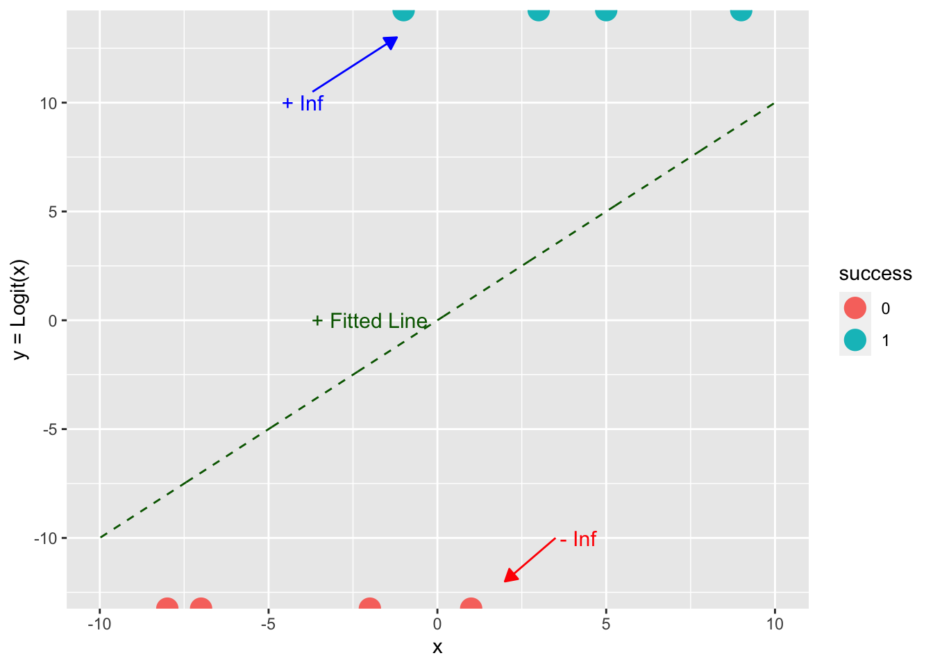
What does this mean for the residuals??
- All the \(Y = \text{Logit}(X)\) values are \(\pm\,\infty\) so we can’t calculate \((\hat{y}_i - y)^2.\)
Thus we will use Maximum Likelihood Estimation.
For any set of \(\beta_0, \beta_1, \ldots, \beta_p\), define the likelihood as:
\[ \text{Likelihood} = \text{Probability of Observing the original } y_i \text{ with their values of 0 or 1}. \]
We assume the \(y_i\) are independent, so we can calculate the individual probabilities and multiply them together.
- This gives us a Likelihood Function for our estimates.
\[ \mathrm{L}(\beta_0, \beta_1, \ldots, \beta_p) = \prod_{i = 1}^{n} \underbrace{p_i^{y_i}}_{\text{Prob }y_i=1}\underbrace{(1-p_i)^{1-y_i}}_{\text{ Prob }y_i = 0} \tag{4.7}\]
Note what happens for \(y_i = 1\) and \(y_i =0\).
We can rewrite Equation 4.7 using Equation 4.6 for the logistic function as
\[ \begin{align} \mathrm{L}(\beta_0, \beta_1, \ldots, \beta_p) &= \prod_{i = 1}^{n} \underbrace{p_i^{y_i}}_{\text{Prob }y_i=1}\underbrace{(1-p_i^{1-y_i})}_{\text{ Prob }y_i = 0} \\ \mathrm{L}(\beta_0, \beta_1, \ldots, \beta_p) &= \prod_{i = 1}^{n}\left( \frac{e^{\beta_0 + \beta_1X_1 + \ldots, + \beta_pX_p}} {(1 + e^{\beta_0 + \beta_1X_1 + \ldots, + \beta_pX_p})}\right)^{y_i} \left( \frac{1}{(1 + e^{\beta_0 + \beta_1X_1 + \ldots, + \beta_pX_p})}\right)^{1-y_i} \end{align} \tag{4.8}\]
R will try to maximize Equation 4.8 by finding the values for the \(\beta\)s that are most consistent with the observed values.
- R takes the logit of this expression and estimates \(\beta_j\) parameters for an initial fitted line in the logit space (Figure 4.4).
- R then projects the \(x_i\) onto the fitted line in logit space to find the \(\text{Logit}(\hat{y}_i)\) on the \(\text{Logit}(Y)\) axis.
- R then transforms the \(\text{Logit}(\hat{y}_i)\) values back to the probability space using Equation 4.3 to calculate likelihood value using Equation 4.8.
- There is no closed-form simple solution to Equation 4.8 as in OLS so software packages use an iterative method to converge on the optimal solution.
- R then updates the estimated \(\beta_j\) parameters of the fitted line in the logit space, in a sense “rotating the line” in Figure 4.4, doing the projections onto the new line to get the new \(\text{Logit}(\hat{y}_i)\), transforming to probabilities to calculate the new Likelihood value.
- R keeps rotating the line and calculating the likelihood function until it converges (reaches a threshold for minimal change in the likelihood.
- The maximum likelihood function is convex so the iterative method uses a weighted form of the linear regression solutions to calculate the next step in estimating the \(\beta_j\)s which means it usually converges in a few iterations.
- R then provides the estimates for the set of \(\beta_j\) that gives the maximum likelihood and calculates the deviances.
4.8.7 Example of Using R for Logistic Regression
Professor Baron has a data set from a study of 1,594 high school students with values for socio-economic and family factors that may be associated with stress and depression.
| Column | Variable | Notes |
|---|---|---|
| 1 | Participant’s identification number | |
| Predictors | ||
| 2 | Gender | Female or Male |
| 3 | Guardian status | 0 = does not live with both natural parents, 1 = lives with both natural parents |
| 4 | Community Cohesion Score: how strongly the participant is connected to the community | 16-80 |
| Response variables | ||
| 5 | Total Depression Score | 0 - 60 |
| 6 | Clinical Diagnosis of Major Depression (or the clinical sample of patients only | 1 = positive diagnosis, 0 = negative diagnosis |
We are interested in predicting the probability of a Clinical Diagnosis of Major Depression based on the possible predictors of Gender, Guardian Status, and Community Cohesion Score.
4.8.7.1 Get and Review the Data
- Read in the data from the following url (https://raw.githubusercontent.com/rressler/data_raw_courses/main/depression_data.csv).
- Use
glimpse()andsummary()to look at the data.
Show code
Rows: 3,189
Columns: 6
$ ID               <dbl> 1, 2, 3, 4, 5, 6, 7, 8, 9, 10, 11, 12, 13, 14, 15, 16…
$ Gender           <chr> "Male", "Male", "Male", "Female", "Male", "Female", "…
$ Guardian_status  <dbl> 1, 1, 0, 1, 0, 1, 1, 0, 1, 0, 1, 0, 0, 1, 1, 1, 1, 0,…
$ Cohesion_score   <dbl> 80.0, 57.1, 36.3, 44.0, 46.0, 40.0, 60.0, 64.0, 76.0,…
$ Depression_score <dbl> 3, 17, 17, 17, 19, 31, 26, 2, 10, 30, 17, 6, 3, 3, 18…
$ Diagnosis <dbl> NA, NA, NA, NA, NA, NA, NA, NA, NA, 0, NA, NA, 0, NA,… ID Gender Guardian_status Cohesion_score
Min. : 1 Length:3189 Min. :0.0000 Min. :16.00
1st Qu.: 800 Class :character 1st Qu.:0.0000 1st Qu.:48.00
Median :1597 Mode :character Median :1.0000 Median :58.00
Mean :1597 Mean :0.5177 Mean :56.24
3rd Qu.:2394 3rd Qu.:1.0000 3rd Qu.:66.00
Max. :3191 Max. :1.0000 Max. :80.00
Depression_score Diagnosis
Min. : 0.00 Min. :0.0000
1st Qu.: 8.00 1st Qu.:0.0000
Median :14.00 Median :0.0000
Mean :15.56 Mean :0.1572
3rd Qu.:21.00 3rd Qu.:0.0000
Max. :54.00 Max. :1.0000
NA's :2731 It appears not all students were diagnosed so Diagnosis has a lot of NAs. Let’s get rid of them using drop_na() for the specific variable.
Rows: 458
Columns: 6
$ ID               <dbl> 10, 13, 28, 30, 40, 45, 47, 78, 79, 87, 102, 105, 117…
$ Gender           <chr> "Female", "Male", "Male", "Male", "Female", "Male", "…
$ Guardian_status  <dbl> 0, 0, 1, 0, 0, 0, 0, 0, 1, 0, 1, 0, 0, 0, 0, 0, 0, 0,…
$ Cohesion_score   <dbl> 69.0, 72.0, 78.0, 56.5, 28.0, 62.0, 43.0, 29.0, 54.0,…
$ Depression_score <dbl> 30, 3, 9, 12, 46, 15, 35, 54, 33, 21, 8, 46, 44, 32, …
$ Diagnosis <dbl> 0, 0, 0, 0, 0, 1, 0, 1, 1, 0, 0, 1, 1, 1, 1, 0, 0, 0,… ID Gender Guardian_status Cohesion_score
Min. : 10.0 Length:458 Min. :0.0000 Min. :16.00
1st Qu.: 884.2 Class :character 1st Qu.:0.0000 1st Qu.:42.00
Median :1720.0 Mode :character Median :0.0000 Median :51.10
Mean :1686.7 Mean :0.4913 Mean :51.78
3rd Qu.:2580.2 3rd Qu.:1.0000 3rd Qu.:62.00
Max. :3182.0 Max. :1.0000 Max. :80.00
Depression_score Diagnosis
Min. : 0.00 Min. :0.0000
1st Qu.:12.00 1st Qu.:0.0000
Median :23.00 Median :0.0000
Mean :22.86 Mean :0.1572
3rd Qu.:32.00 3rd Qu.:0.0000
Max. :54.00 Max. :1.0000 It looks like Diagnosis and Gender should be categorical so we could convert to factors but let’s wait for a few minutes.
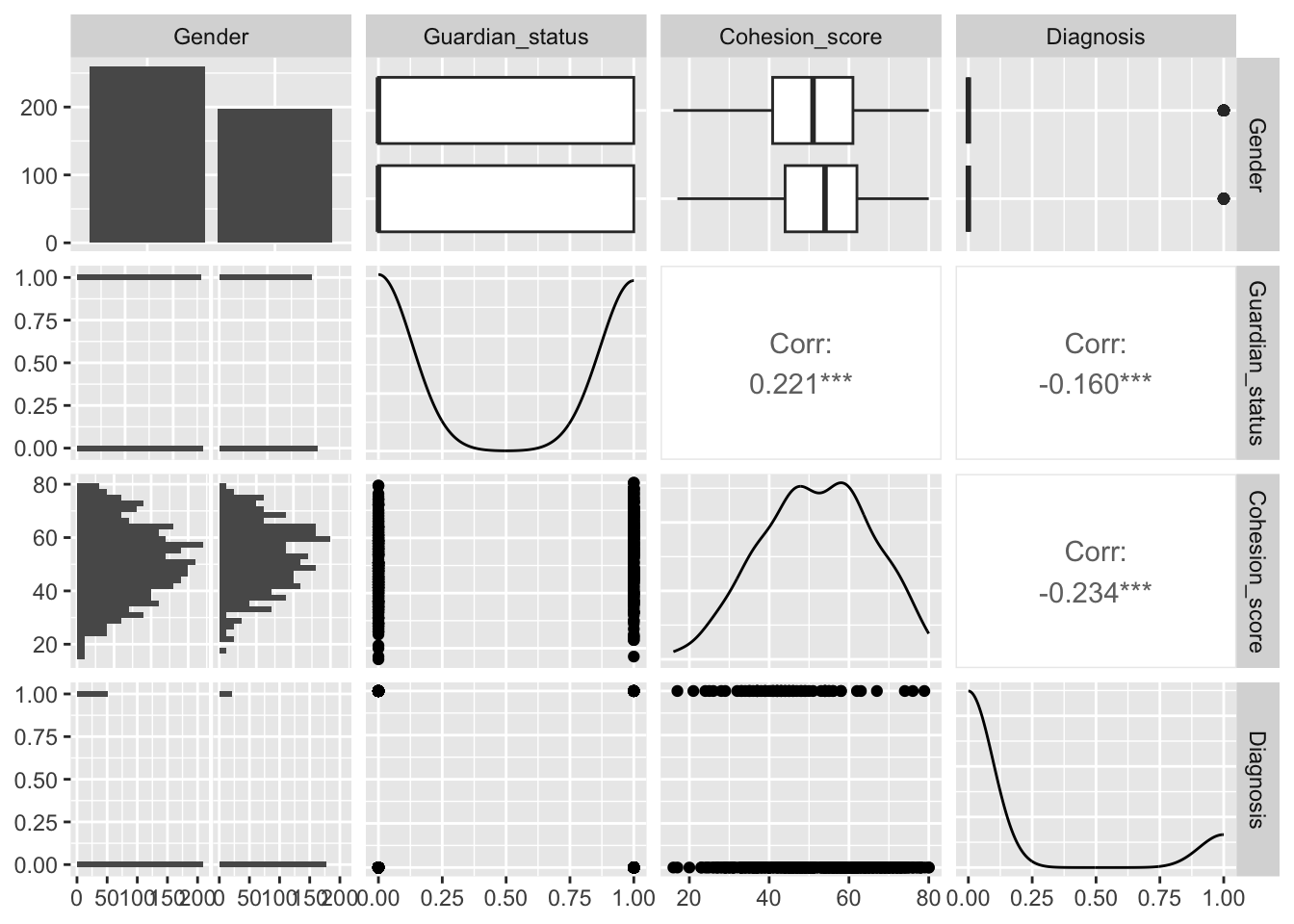
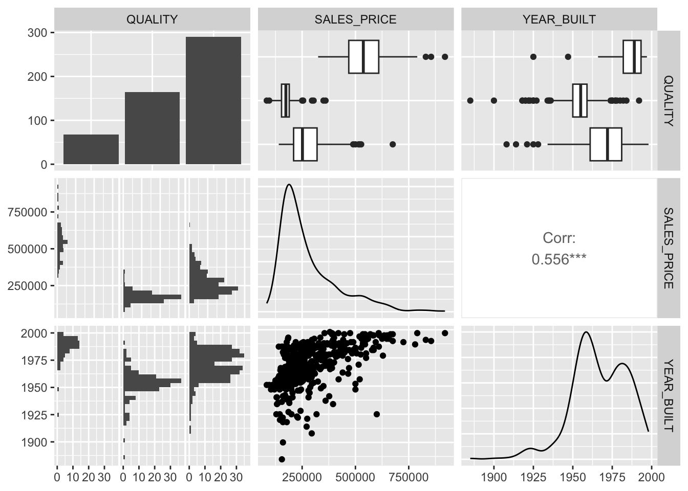
Let’s use GGally::ggpairs() to look at our four variables of interest.
4.8.7.2 Build and Interpret Results for a Logistic Regression Model in R
We can use the stats::glm() function to run a logistic regression model.
The default for the family = argument is “gaussian” which means this default version of glm() runs a standard OLS model where \(Y\) is NOT categorical, just a double, with values of 0, 1.
The summary() of a glm() output object looks similar to a lm() output object with a few differences at the bottom.
Call:
glm(formula = Diagnosis ~ Gender + Cohesion_score + Guardian_status,
    data = depr)

Coefficients:
                 Estimate Std. Error t value Pr(>|t|)
(Intercept)      0.512988   0.065434   7.840 3.25e-14 ***
GenderMale      -0.080745   0.033179  -2.434   0.0153 *
Cohesion_score  -0.005386   0.001241  -4.340 1.76e-05 ***
Guardian_status -0.085443   0.033627  -2.541   0.0114 *
---
Signif. codes:  0 '***' 0.001 '**' 0.01 '*' 0.05 '.' 0.1 ' ' 1

(Dispersion parameter for gaussian family taken to be 0.123044)

    Null deviance: 60.681  on 457  degrees of freedom
Residual deviance: 55.862  on 454  degrees of freedom
AIC: 346.12

Number of Fisher Scoring iterations: 2
Let’s look at a histogram of the fitted values and the plots of the OLS results.

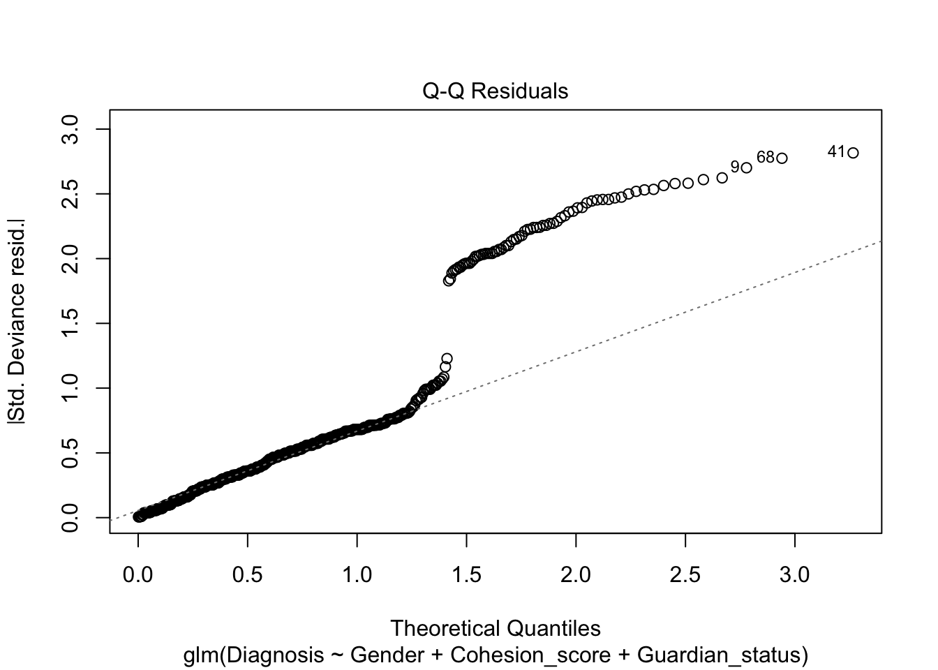
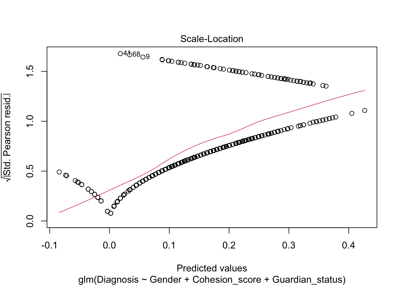
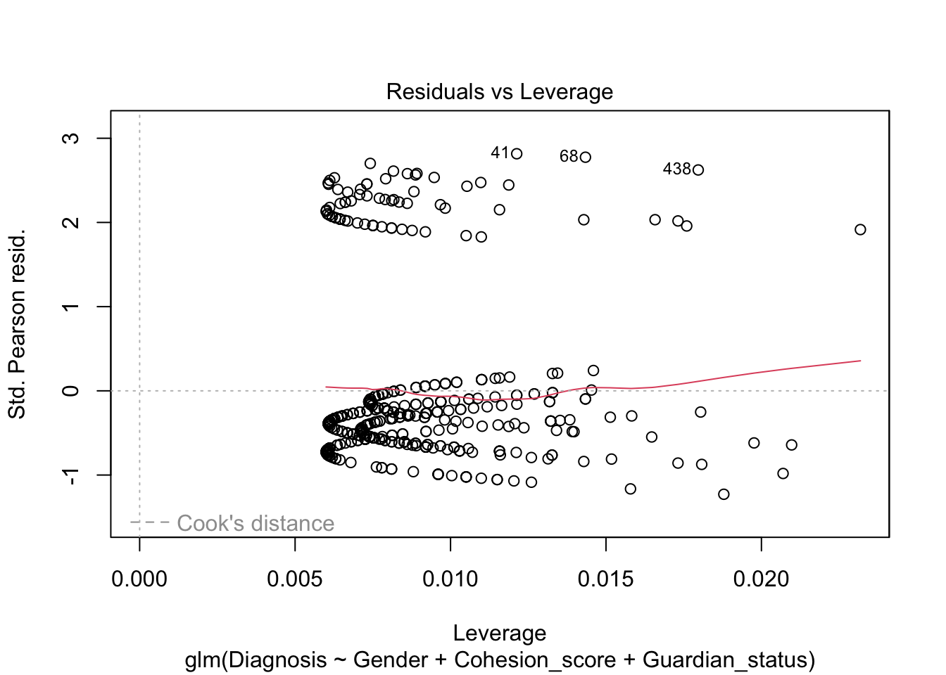
Not very satisfactory; note the predicted probabilities where \(\hat{y}<0.\) Let’s re-run as a logistic regression.
We could convert Gender and Diagnosis to factors, but R will treat response variables with binary values (character or numeric) as factors when using Logistic Regression, so it will create dummy variables for \(Y\) behind the scenes.
Show code
Call:
glm(formula = Diagnosis ~ Gender + Cohesion_score + Guardian_status,
    family = binomial, data = depr)

Coefficients:
                Estimate Std. Error z value Pr(>|z|)
(Intercept)      1.00832    0.50478   1.998  0.04577 *
GenderMale      -0.68744    0.28848  -2.383  0.01718 *
Cohesion_score  -0.04358    0.01046  -4.167 3.09e-05 ***
Guardian_status -0.74835    0.28602  -2.616  0.00889 **
---
Signif. codes:  0 '***' 0.001 '**' 0.01 '*' 0.05 '.' 0.1 ' ' 1

(Dispersion parameter for binomial family taken to be 1)

    Null deviance: 398.47  on 457  degrees of freedom
Residual deviance: 360.38  on 454  degrees of freedom
AIC: 368.38

Number of Fisher Scoring iterations: 5
Three slopes. All are negative. How do we interpret the slopes?
-
Increasing the value of \(X\) with a negative slope will reduce the probability.
- Males have lower probability of depression than females.
- Increasing cohesion will lower the probability of depression.
- Having a parent or guardian will lower the probability of depression.
We can plot the fitted values using a histogram.
Show code
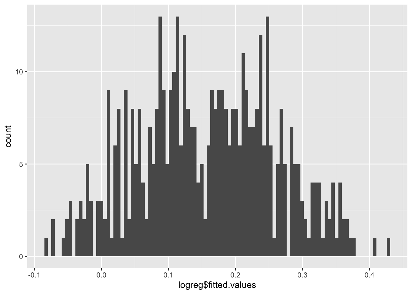
Now the predicted probabilities are \(0<\hat{y}<1.\)
Note, the plot() defaults for the residuals are still not very useful.
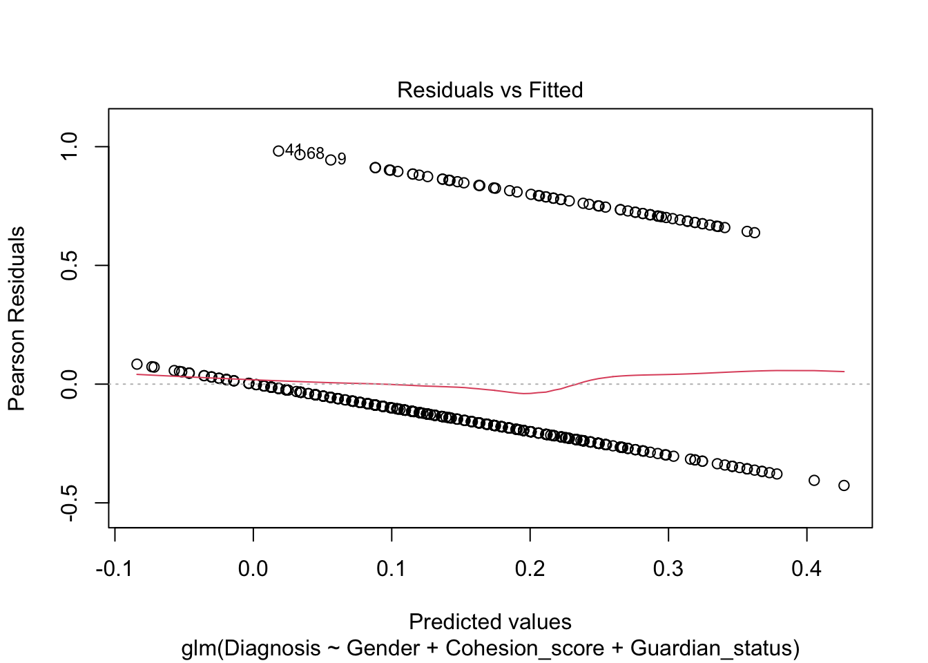


We see a measure of “Deviance” in bottom of the summary. What is this instead of \(R^2\)?
4.8.8 Deviance
Deviance is a measure of the goodness of fit used in general linear models.
- It can be considered a replacement for, or extension of, the concept of Error Sum of Squares (aka SSE or Residual Sum of Squares (RSS)) when using maximum likelihood methods.
- There are multiple approaches to using and calculating deviance. We are using the one used in R.
For logistic regression, deviance is considered the sum of the individual deviance for each \(\hat{y}_i\) , \(D(y, \hat{y}) = \sum_i d(y_i, \hat{y}_i)\).
- The Total Deviance for a fit model, where the likelihood \(L\) has been maximized, is calculated using the following formula :
\[ D(y, \hat{y}) = D_\text{saturated}-2\,\ln\left(\mathrm{L}(\hat{\beta_0}, \hat{\beta}_1, \ldots, \hat{\beta}_p)\right) \tag{4.9}\]
- The \(D_\text{saturated}\) is the deviance for a perfect saturated model where every point as an individual fit. It is usually scaled so \(D_\text{saturated}=0.\)
- The 2 in Equation 4.9 is needed so the distribution of the deviance is approximately \(\chi^2\).
- The log is used to help scale the results.
The Null Deviance is the calculated deviance for the Null (Dull) Hypothesis model with only an intercept term \(\hat{\beta}_0\) and assuming all the other \(\beta_i = 0\) i.e., they have no predictive power in explaining the variance of the logit(\(y\)).
The Residual Deviance is deviance for the fitted model, with the best fitting \(\hat{\beta}_i.\)
The lower the Residual Deviance the better the fit.
Since the calculated deviance is always a comparison with a perfect, saturated model, the Null Hypothesis is that if all the assumptions are true, the fitted model is a good fit, close to “perfect”.
Thus we want the \(p\)-value to be close to 1 so there is no evidence to reject the model.
- The deviances follow a \(\chi^2\) distribution with \(df = n - p\) degrees of freedom.
- We can use this with the output of the fitted model object to calculate a \(p\)-value for the Null Hypothesis being true.
[1] 0.9774268[1] 0.9995629The closer the \(p\)-value is to 1, the closer the model corresponds to a “perfect” saturated model.
4.8.9 Predicting New Values
We have a model, so we can predict for new cases using the estimates produced by our model.
Call:
glm(formula = Diagnosis ~ Gender + Cohesion_score + Guardian_status,
    family = binomial, data = depr)

Coefficients:
                Estimate Std. Error z value Pr(>|z|)
(Intercept)      1.00832    0.50478   1.998  0.04577 *
GenderMale      -0.68744    0.28848  -2.383  0.01718 *
Cohesion_score  -0.04358    0.01046  -4.167 3.09e-05 ***
Guardian_status -0.74835    0.28602  -2.616  0.00889 **
---
Signif. codes:  0 '***' 0.001 '**' 0.01 '*' 0.05 '.' 0.1 ' ' 1

(Dispersion parameter for binomial family taken to be 1)

    Null deviance: 398.47  on 457  degrees of freedom
Residual deviance: 360.38  on 454  degrees of freedom
AIC: 368.38

Number of Fisher Scoring iterations: 5
We can get the logit manually, using Equation 4.5 as follows:
\[ \begin{align} \text{logit}(Y) = \ln\frac{p}{1-p} &= \beta_0 + \beta_1 X_1 + \beta_2 X_2 + \beta_3 X_3 \\ &= 1.00832 - 0.68744 * \text{GenderMale} - 0.04358 * \text{Cohesion score}- 0.74835 * \text{Guardian status} \\ \end{align} \]
If we predict for a Male, living with parents and cohesion score of 20, we get a logit (aka log odds) of
Using R we enter the new data into the predict() function.
Show code
       1
-1.29902
This result is the logit of the probability.
We could convert to the probability for \(Y = 1\) using Equation 4.3 as follows:
\[ \begin{align} p &= \frac{e^{\beta_0 + \beta_1 X_1 + \beta_2 X_2 + \beta_3 X_3}}{1 + e^{\beta_0 + \beta_1 X_1 + \beta_2 X_2 + \beta_3 X_3}} \\ &= \frac{e^{1.00832 - 0.68744 * \text{GenderMale}- 0.04358 * \text{Cohesion score}- 0.74835 * \text{Guardian status}}}{1 + e^{1.00832 - 0.68744 * \text{GenderMale} - 0.04358 * \text{Cohesion score}- 0.74835 * \text{Guardian status}}} \\ \end{align} \]
- With a result of
Or, we can use the predict() function’s argument type = "response" to have R transform the output into the original space of the \(Y\).
Show code
      1
0.21433 Show code
        1
0.3516983
Show code
       1
0.534139
What can we do to help college students?
Assuming fixed gender and parental/guardian situations, focus on Cohesion Score.
4.8.10 Converting Logistic Regression Probabilities into Predictions (Classifications)
Logistic Regression is a useful parametric classification method for binary response variables where we are trying to estimate the probability of a success.
- Categorical, binary, response is represented by dummy variable with values 0 or 1.
- The Logistic Regression Model from Equation 4.6 can be seen as:
\[ E[Y] = p(Y = 1|X) = p(X) = \frac{e^{\beta_0 + \beta_1X + \ldots, \beta_pX_p}}{1 + e^{\beta_0 + \beta_1X + \ldots, \beta_pX_p}} \]
- All \(\beta_j\) are estimated by the method of Maximum Likelihood Estimate (MLE), not Least Squares.
- MLE means choosing values for the parameters (\(\beta\)s) that make what we observe in the \(Y\) and \(X\) have the highest probability of occurring.
- We get estimates for \(\hat{\beta}_j\) which results in \(\hat{p}(Y = 1)\) but this is a probability of an outcome, not a prediction.
4.8.11 Convert \(p(Y=1)\) into a Classification Prediction
There are several ways to convert to a classification:
- We could just say if \(\hat{p}(Y = 1) \geq .5\) predict a success. That approach is not robust and it leaves out information about the risks of the outcomes.
- We could tune the model to select the “best” threshold.
- We could use a Decision-theoretic approach which considers benefits and risks or costs in terms of gains and losses. We’ll discuss this in a few minutes.
4.8.12 Tuning the Model to Select a Threshold: Example with Titanic Data
Let’s consider data about the outcomes of the ill-fated voyage of the RMS Titanic as an example (Trailer Clip). The ship had 2,207 passengers and crew and only 711 survived.
The {DALEX} package’s titanic data set includes a complete list of the passengers and crew. You can get it from the package or from https://raw.githubusercontent.com/rressler/data_raw_courses/main/titanic_dalex.csv/
Show code
Rows: 2,207
Columns: 9
$ gender   <chr> "male", "male", "male", "female", "female", "male", "male", "…
$ age      <dbl> 42.0000000, 13.0000000, 16.0000000, 39.0000000, 16.0000000, 2…
$ class    <chr> "3rd", "3rd", "3rd", "3rd", "3rd", "3rd", "2nd", "2nd", "3rd"…
$ embarked <chr> "Southampton", "Southampton", "Southampton", "Southampton", "…
$ country  <chr> "United States", "United States", "United States", "England",…
$ fare     <dbl> 7.1100, 20.0500, 20.0500, 20.0500, 7.1300, 7.1300, 24.0000, 2…
$ sibsp    <dbl> 0, 0, 1, 1, 0, 0, 1, 1, 0, 0, 0, 0, 1, 0, 0, 0, 0, 0, 0, 0, 0…
$ parch    <dbl> 0, 2, 1, 1, 0, 0, 0, 0, 0, 0, 0, 0, 0, 1, 1, 0, 0, 0, 0, 0, 0…
$ survived <chr> "no", "no", "no", "yes", "yes", "yes", "no", "yes", "yes", "y… gender age class embarked
Length:2207 Min. : 0.1667 Length:2207 Length:2207
Class :character 1st Qu.:22.0000 Class :character Class :character
Mode :character Median :29.0000 Mode :character Mode :character
Mean :30.4367
3rd Qu.:38.0000
Max. :74.0000
NA's :2
country fare sibsp parch
Length:2207 Min. : 0.000 Min. :0.0000 Min. :0.0000
Class :character 1st Qu.: 0.000 1st Qu.:0.0000 1st Qu.:0.0000
Mode :character Median : 7.151 Median :0.0000 Median :0.0000
Mean : 19.773 Mean :0.2972 Mean :0.2294
3rd Qu.: 20.111 3rd Qu.:0.0000 3rd Qu.:0.0000
Max. :512.061 Max. :8.0000 Max. :9.0000
NA's :26 NA's :10 NA's :10
survived
Length:2207
Class :character
Mode :character
  no  yes
1496 711 # A tibble: 1 × 9
gender age class embarked country fare sibsp parch survived
<int> <int> <int> <int> <int> <int> <int> <int> <int>
1 0 2 0 0 81 26 10 10 0Variable Notes
-
pclass: A proxy for socio-economic status (SES): 1st = Upper, 2nd = Middle, 3rd = Lower. -
age: Age is fractional if less than 1. If the age is estimated, is it in the form of xx.5. -
sibsp: Sibling = brother, sister, stepbrother, stepsister; Spouse = husband, wife (mistresses and fiancés were ignored) -
parch: Parent = mother, father; Child = daughter, son, stepdaughter, or stepson. Some children traveled only with a nanny, thereforeparch=0for them. -
embarked: Port of embarkation (C = Cherbourg, Q = Queenstown, S = Southampton)
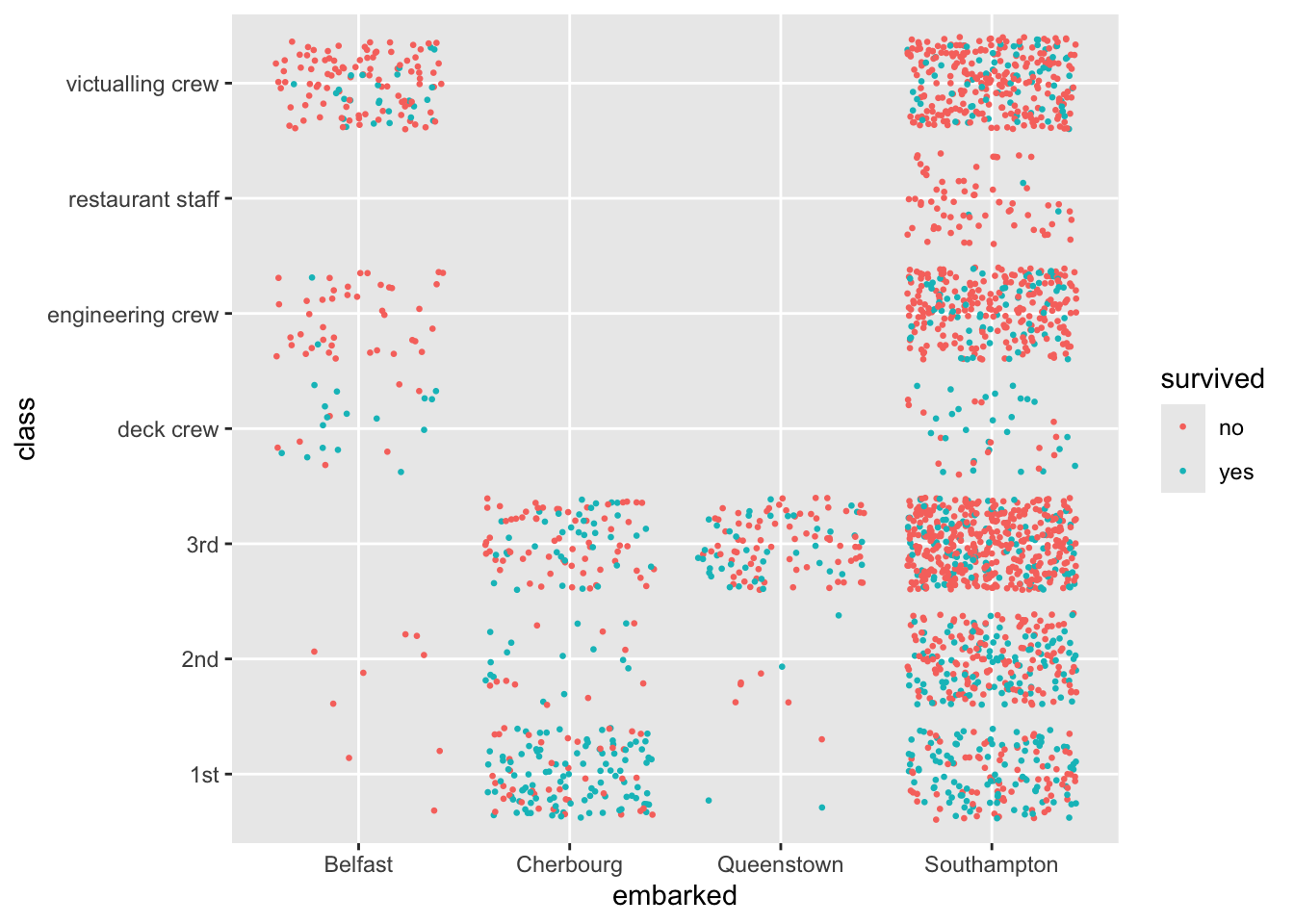
Let’s plot some of the data.
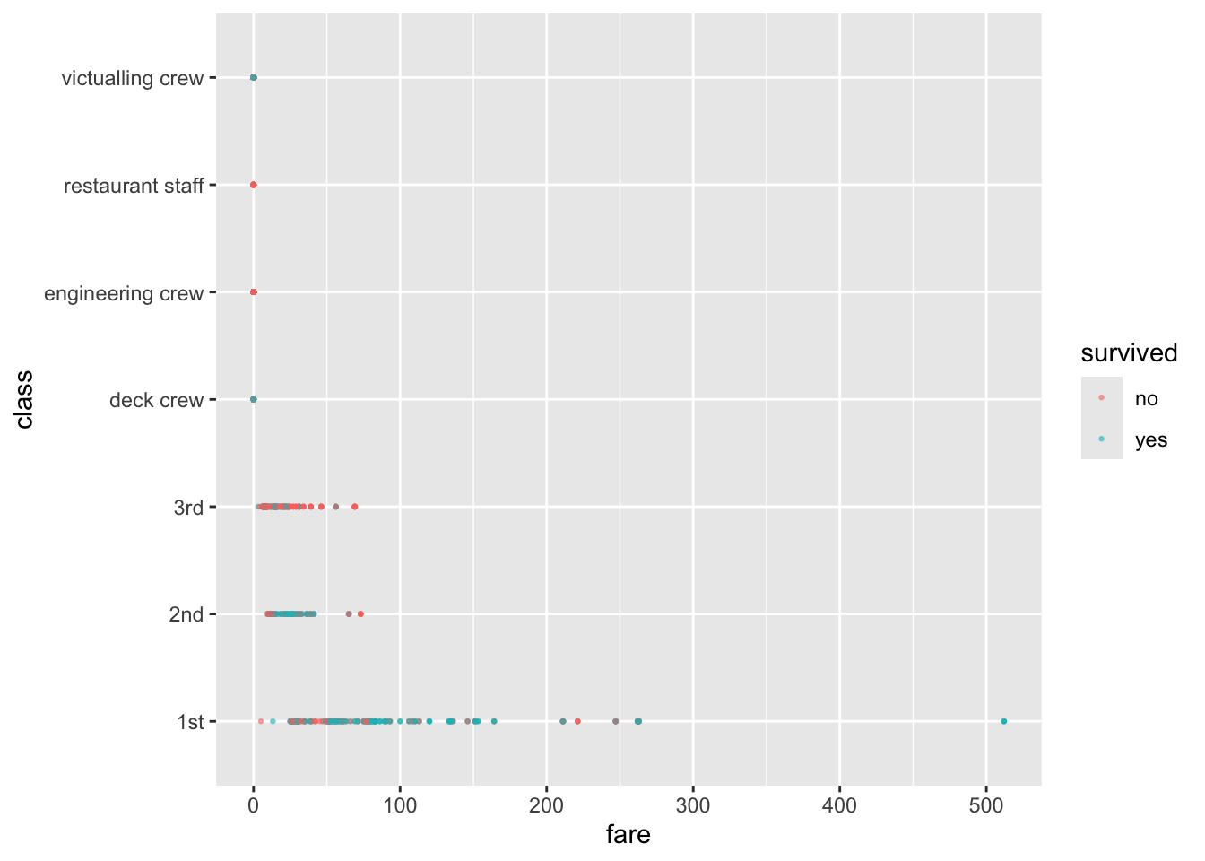
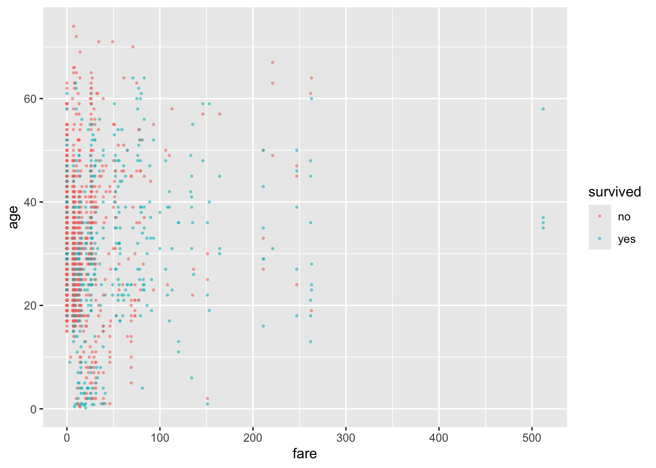
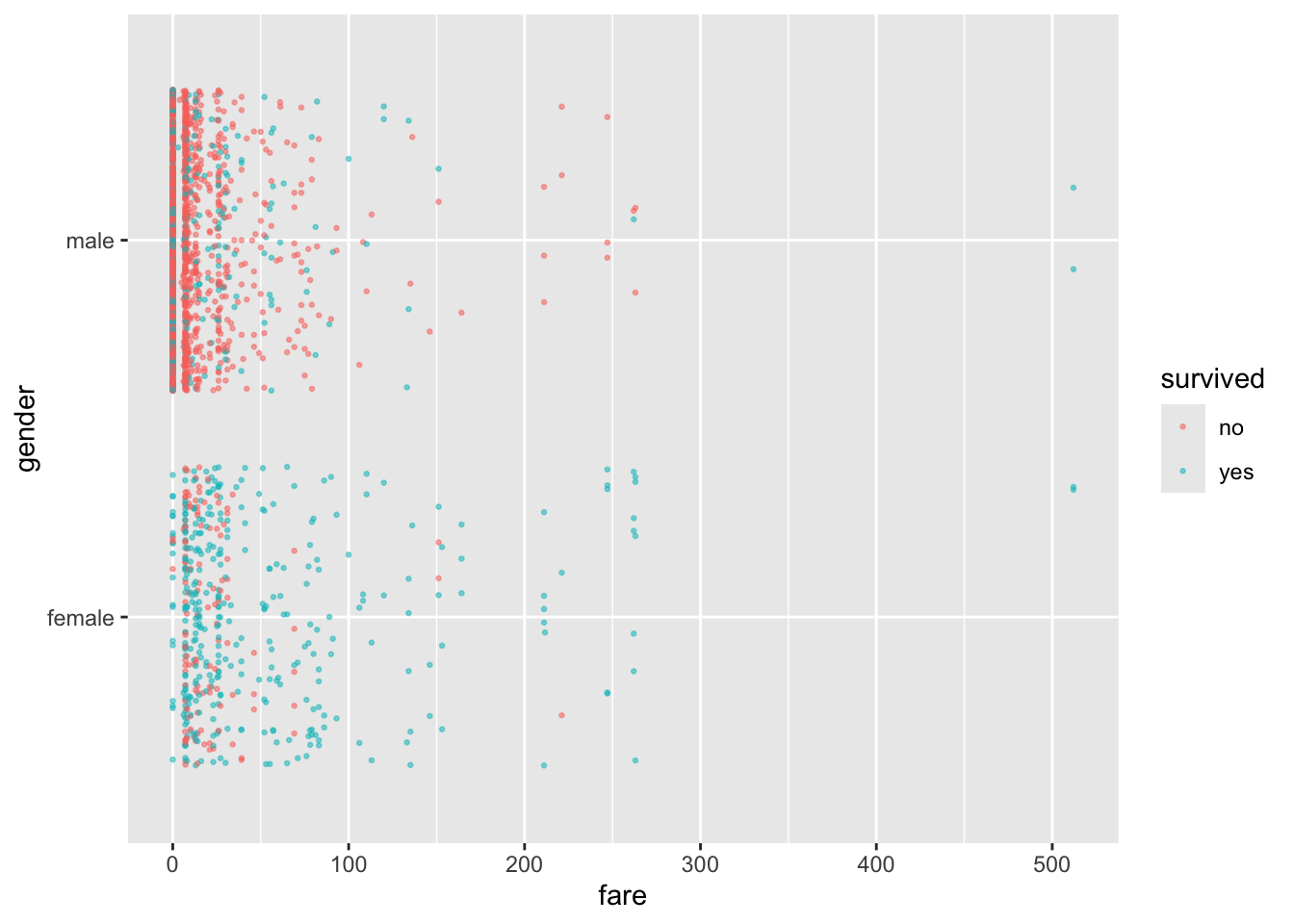
Let’s create an initial logistic regression model using glm().
logreg <- glm(as.factor(survived) ~ age + gender + class + fare + embarked,
              data = titanic, family = "binomial")
summary(logreg)
Call:
glm(formula = as.factor(survived) ~ age + gender + class + fare +
    embarked, family = "binomial", data = titanic)

Coefficients:
                        Estimate Std. Error z value Pr(>|z|)
(Intercept)            3.1774860  0.4078547   7.791 6.66e-15 ***
age                   -0.0317519  0.0051464  -6.170 6.84e-10 ***
gendermale            -2.5835288  0.1486233 -17.383  < 2e-16 ***
class2nd              -1.1103673  0.2455656  -4.522 6.14e-06 ***
class3rd              -2.2245019  0.2425002  -9.173  < 2e-16 ***
classdeck crew         1.0555309  0.3449171   3.060 0.002212 **
classengineering crew -0.9877114  0.2573233  -3.838 0.000124 ***
classrestaurant staff -3.2304528  0.6489321  -4.978 6.42e-07 ***
classvictualling crew -1.1119024  0.2540240  -4.377 1.20e-05 ***
fare                  -0.0008393  0.0017167  -0.489 0.624923
embarkedCherbourg      0.7398312  0.2867817   2.580 0.009887 **
embarkedQueenstown     0.2568812  0.3322973   0.773 0.439495
embarkedSouthampton    0.1106313  0.2152828   0.514 0.607330
---
Signif. codes:  0 '***' 0.001 '**' 0.01 '*' 0.05 '.' 0.1 ' ' 1

(Dispersion parameter for binomial family taken to be 1)

    Null deviance: 2749.3  on 2178  degrees of freedom
Residual deviance: 2038.9  on 2166  degrees of freedom
  (28 observations deleted due to missingness)
AIC: 2064.9

Number of Fisher Scoring iterations: 5
What can we say about the significance of the slopes?
-
fareandembarkeddo not seem significant. Why do you think that is?
Let’s predict for the entire data set and look at the summary().
   Min. 1st Qu.  Median    Mean 3rd Qu.    Max.
 0.0166  0.1338  0.2210  0.3254  0.5182  0.9670
We can make a reduced model without fare and embarked.
- When we do this, recall that
agehad twoNAs so we will remove those rows before running our model.
titanic <- tidyr::drop_na(titanic, age)
logreg <- glm(as.factor(survived) ~ age + gender + class,
              data = titanic, family = "binomial")
summary(logreg)
Call:
glm(formula = as.factor(survived) ~ age + gender + class, family = "binomial",
    data = titanic)

Coefficients:
                       Estimate Std. Error z value Pr(>|z|)
(Intercept)            3.481343   0.276971  12.569  < 2e-16 ***
age                   -0.032148   0.005088  -6.319 2.63e-10 ***
gendermale            -2.608988   0.144603 -18.042  < 2e-16 ***
class2nd              -1.300607   0.210413  -6.181 6.36e-10 ***
class3rd              -2.275826   0.197398 -11.529  < 2e-16 ***
classdeck crew         0.862530   0.297321   2.901  0.00372 **
classengineering crew -1.157325   0.200923  -5.760 8.41e-09 ***
classrestaurant staff -3.392692   0.628902  -5.395 6.87e-08 ***
classvictualling crew -1.297206   0.190148  -6.822 8.97e-12 ***
---
Signif. codes:  0 '***' 0.001 '**' 0.01 '*' 0.05 '.' 0.1 ' ' 1

(Dispersion parameter for binomial family taken to be 1)

    Null deviance: 2772.6  on 2204  degrees of freedom
Residual deviance: 2071.0  on 2196  degrees of freedom
AIC: 2089

Number of Fisher Scoring iterations: 5
Let’s predict for Rose and Jack from the movie.
        1
0.9495412 1
0.1111957 1
0.2491098 1
0.5491511 Let’s tune the model by creating training and testing data and then searching for the threshold that reduces the mis-classification rate.
Create the model using the training data and the predictions with the test data.
logreg <- glm(as.factor(survived) ~ age + gender + class,
              data = titanic[Z,], family = "binomial")
summary(logreg)
Call:
glm(formula = as.factor(survived) ~ age + gender + class, family = "binomial",
    data = titanic[Z, ])

Coefficients:
                       Estimate Std. Error z value Pr(>|z|)
(Intercept)            3.317224   0.374814   8.850  < 2e-16 ***
age                   -0.031366   0.007075  -4.433 9.28e-06 ***
gendermale            -2.445826   0.201992 -12.109  < 2e-16 ***
class2nd              -1.278162   0.294380  -4.342 1.41e-05 ***
class3rd              -2.175948   0.266656  -8.160 3.35e-16 ***
classdeck crew         1.027517   0.431904   2.379 0.017358 *
classengineering crew -1.153568   0.275801  -4.183 2.88e-05 ***
classrestaurant staff -3.010567   0.788051  -3.820 0.000133 ***
classvictualling crew -1.272025   0.258695  -4.917 8.78e-07 ***
---
Signif. codes:  0 '***' 0.001 '**' 0.01 '*' 0.05 '.' 0.1 ' ' 1

(Dispersion parameter for binomial family taken to be 1)

    Null deviance: 1379.1  on 1101  degrees of freedom
Residual deviance: 1059.4  on 1093  degrees of freedom
AIC: 1077.4

Number of Fisher Scoring iterations: 5Let’s check for a range of thresholds between 0 and 1.
- We already have the predictions, we just need to calculate the results by comparing to each threshold.
[1] 101[1] 0.00 0.01 0.02 0.03 0.04 0.05Show code
TPR <-  FPR <- err.rate <- rep(0, length(threshold))

for (i in seq_along(threshold)) {
Yhat <- rep(NA_character_, nrow(titanic[-Z,]))
Yhat <-  ifelse(Prob >= threshold[[i]], "yes", "no")

err.rate[i] <- mean(Yhat != titanic[-Z,]$survived)
TPR[[i]] <- sum(Yhat == "yes" & titanic[-Z,]$survived == "yes") /
  sum(titanic[Z,]$survived == "yes")
FPR[[i]] <- sum(Yhat == "yes" & titanic[-Z,]$survived == "no") /
  sum(titanic[-Z,]$survived == "no")
}
Now we have the data to plot the error rate.
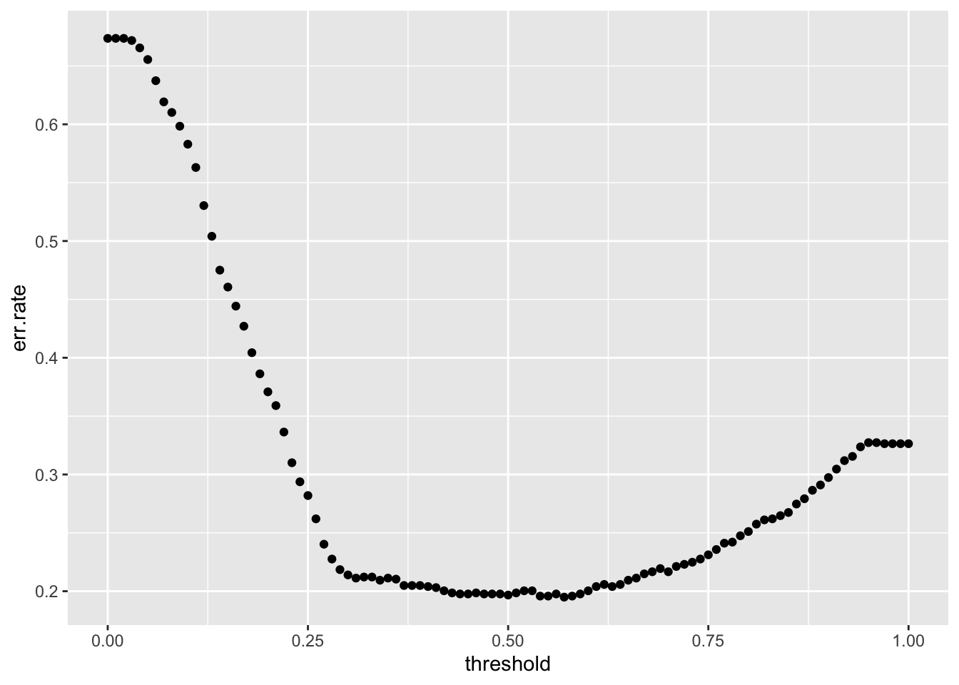
 no yes
751 351 [1] 0.3185118So a low threshold says everyone will survive when in fact only 31.85% of our training data survived.
What is the best threshold?
[1] 58[1] 0.57[1] 0.1949229Let’s reset our Yhat to the threshold that minimizes the error rate and create a confusion matrix .
Show code
Yhat   no yes
  no  690 162
  yes  53 198
So a threshold of 0.57 for this sample is correct and we predict 80.51% correctly
We can also plot an ROC Curve for the training data.
Show code
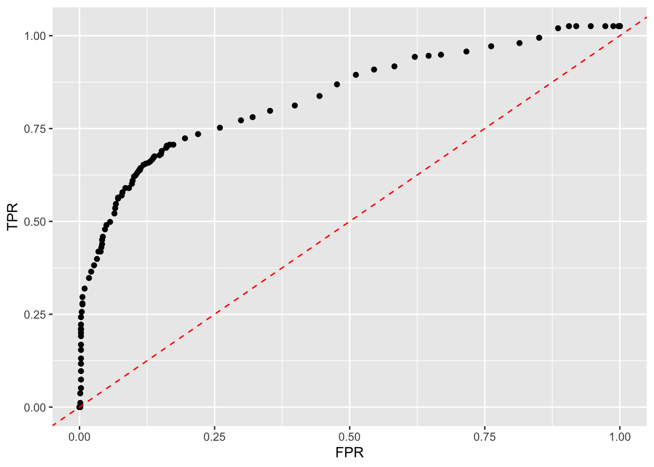
Note the top right of the curve depicts low thresholds since our data has a low rate of survival.
- The lower the threshold, the more likely to say someone survived so you will catch all the actual survivors, but, generate a lot of False Positives.
- The higher the threshold, the more likely to say someone died, so will not get all of the survivors (a lower True Positive Rate) but, have lower chance of a False Positive.
Show code
ggplot(tibble(TPR,FPR),
       aes(FPR, TPR)) +
  geom_point() +
  geom_point(aes(FPR[11], TPR[11]),
             color = "red", size = 5) +
  annotate("text", x = .85, y = .8, label = "Low Threshold", color = "red") +
geom_point(aes(FPR[90], TPR[90]),
             color = "blue", size = 5) +
  annotate("text", x = .2, y = .08, label = "High Threshold", color = "blue") +
geom_point(aes(FPR[51], TPR[51]),
             color = "darkgreen", size = 5) +
  annotate("text", x = .3, y = .58, label = "Best Threshold", color = "darkgreen")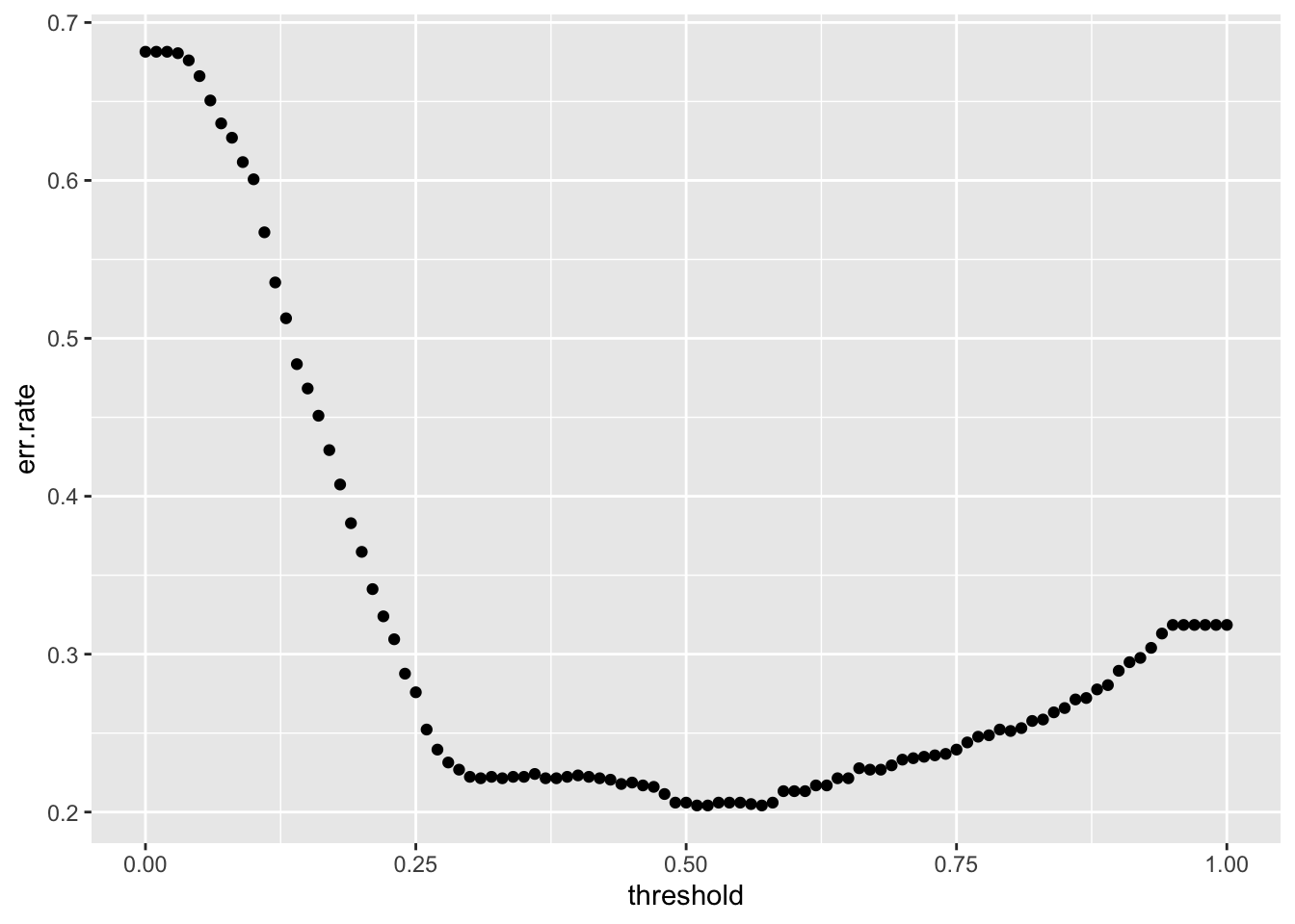
4.8.13 Determining Thresholds Using Loss Functions - a Decision Theoretic Approach
Let’s assume the actual value is either \(Y\) = 1, with probability \(p\), or \(Y=0\) with probability \((1-p)\). We then have the choice of predicting \(\hat{Y} = 1\) or \(\hat{Y} = 0\) based on a threshold for \(p\) that we get to choose. We want to choose a threshold for \(p\) that minimizes our decision risk or the expected loss from our where we set our threshold.
To structure our approach, let’s create a 2 x 2 matrix of the actual values and our possible predictions \(\hat{Y}\) where the intersection is one of our four possible outcomes.
We then enter the associated loss for each outcome, based on whether \(\hat{Y} = Y.\)
When we predict correctly, \(\hat{Y} = Y\), (on the main diagonal from top left to bottom right), the value of the loss function is 0, as we were correct.
-
When we predict incorrectly, \(\hat{Y} \neq Y\), (the off-main diagonal), we represent the loss functions for each error as \(L_0\) and \(L_1\).
- \(L_1\) is the loss associated with a False Positive.
- \(L_2\) is the Loss associated with a False Negative.
Our table looks like the following:
| Loss function | \(Y = 1\) | \(Y= 0\) |
|---|---|---|
| \(\hat{Y} = 1\) | 0 | \(L_1\) |
| \(\hat{Y} = 0\) | \(L_0\) | 0 |
It is not clear that \(L_1 = L_0\) in all situations.
- Consider the choice of a car insurance company. Is the loss the same when they lose a customer (don’t issue a policy) to a safe driver (False Negative) or if they issue a policy to a driver who then has an accident (False Positive)?
In a decision theory approach, we estimate \(p\) with \(\hat{p}\) and want to find a threshold for the probability \(\hat{p}\) so we can create a decision rule to minimize the risk (expected loss) of future predictions.
How do we calculate the risk for each choice from our 2x2 table?
- The actual or true \(p(Y = 1) = p\) (the expected value (mean) of the Bernoulli Distribution).
We define Risk as the Expected Value of the Loss for a prediction (or it may be referred to as the Expected Cost of a prediction).
- Many risk models are 2x2 where they estimate the probability of occurrence for a risk and the effect of the the risk if it happens.
- Organizations develop risk mitigation strategies to minimize one or both dimensions.
- They often consider risks across Cost, Performance, and Schedule.
We want to minimize the Risk (Expected Value of the Loss) over all possible decision choices (our choices are to predict 1, or 0).
- This means we want to minimize the Expected Loss expressed as:
\[ \text{Risk}= E[\text{Loss}] = \sum_{i = Choices}p(\text{Loss value}_i)\times \,\,\text{Loss value}_i \tag{4.10}\]
Equation 4.10 follows the standard approach to calculate the expected value of a discrete random variable; the sum, over all possible values, of the probability of a value \(\times\) that value.
In our example Loss function, Equation 4.10, we have two choices for a prediction (1, or 0), so we can calculate the risk for each choice.
For the choice of \(\hat{y} = 1\), we use the top row of the table to get:
\[\text{Risk}(\hat{y} = 1) = p\times 0 + (1-p)\times L_1 = (1-p)L_1. \tag{4.11}\]
- Equation 4.11 is the risk or expected loss of a False Positive.
For the choice of \(\hat{y} = 0\), we use the second (bottom) row of the table:
\[\text{Risk}(\hat{y} = 0) = = p \times L_0 + (1-p)\times 0 = p L_0 \tag{4.12}\]
- Equation 4.12 is the risk or expected loss of a False Negative.
Given the two choices for our prediction, we can compare their risk values from Equation 4.11 and Equation 4.12.
To minimize our risk, we choose the prediction with the smaller risk value as our prediction.
Combining Equation 4.11 and Equation 4.12, we can create a decision rule to minimize our prediction risk.
\[ \text{Predict } \hat{Y} = 1 \quad \text{ if }\quad (1-p)L_1 < p L_0 \tag{4.13}\]
Equation 4.13 can be read as: Predict 1 when the Risk of a False Positive is less than the Risk of a False Negative.
An equivalent decision rule is: \[ \text{Predict } \hat{Y} = 0 \quad \text{ if }\quad (1-p)L_1 > p L_0 \tag{4.14}\]
Equation 4.14 can be read as: Predict 0 when the Risk of a False Positive is greater than the Risk of a False Negative.
We can manipulate Equation 4.13 to create a ratio of the two expected losses:
\[ \text{Predict } \hat{Y} = 1 \text{ if }\quad \frac{L_1}{L_0} < \frac{p}{1-p} \quad \text{(the odds ratio)} \tag{4.15}\]
We can also interpret Equation 4.15 in terms of decision “guidance” for making a predication:
- Predict \(\hat{y} = 1\) if it has a “small” loss \(L_1\) (if it is wrong), or,
- Predict \(\hat{y} = 1\) if \(p(Y=1)\) is “large”.
We need to define what “small” and “large” mean to create a useful rule.
Let’s look at the case when \(L_1 = L_0\), so there is the same loss for either false prediction (this is what we have already been assuming in previous examples).
- When \(L_1 = L_0\), Equation 4.15 implies “large” is when the odds ratio is larger than 1 or \(1< \frac{p}{1-p}\). When does this happen?
- Let’s do the math …
\[ p \text{ is Large} \iff1 <\frac{p}{1-p} \iff (1-p)< p \iff 1< 2p \iff 1/2 < p. \]
- So, set the threshold for \(\hat{p}\) at \(\hat{p} = 1/2\) and predict \(\hat{y}_i = 1\) for any \(\hat{p}_i \geq 1/2\).
What about when \(L_1 \neq L_0\)?
Let’s assume \(L_1 = 2L_0\); the loss from a false positive is twice as bad as a false negative.
We can use Equation 4.15 to predict \(\hat{y} = 1\) when:
\[ \frac{L_1}{L_0} < \frac{p}{1-p} \iff \frac{2L_0}{L_0} < \frac{p}{1-p} \iff 2 < \frac{p}{1-p} \iff 2-2p < p \iff 2/3<p \]
- So, set the threshold for success at \(\hat{p} = 2/3\) and predict \(\hat{y}_i = 1\) for any \(\hat{p}_i \geq 2/3\).
We are setting the threshold at a specific value of equality and making decisions for values greater than or equal to the threshold. Recall that for continuous random variables, the probability that we will get any specific value is 0 so it does not change the result by using $\geq$.- We are setting a high threshold as the risk of a False Positive is relatively high and we want to minimize them.
What if the Loss for \(L_1 = cL_0\) for some positive constant \(c>0\).
\[ \frac{L_1}{L_0} < \frac{p}{1-p} \iff \frac{cL_0}{L_0} < \frac{p}{1-p} \iff c < \frac{p}{1-p} \iff c-cp < p \iff \frac{c}{1+c}<p \] What happens as \(c\) gets really large and goes to \(\infty\)?
\[ \frac{c}{1+c}\leq p \longrightarrow \frac{c}{c}\leq p \implies 1 \leq p. \] The higher the risk of a false positive to a false negative, the higher the optimal threshold until you never predict \(\hat{y} = 1\).
The ratio of the loss functions for the False Positives and False Negatives will establish the threshold for \(\hat{p}\) to determine when to decide to predict or \(\hat{y_i} = 1\) given a \(\hat{p}_i.\)
You can also extend the analysis to include gains or benefits for correct decisions.
4.8.14 Summary of Logistic Regression
Logistic Regression is a useful method with binary response variable, where \(p(Y=1) = p\) and \(p(Y=0) = (1-p)\)s and we want to predict the conditional probability \(\hat{p}=p(Y = 1|X)\).
We saw the method has s few major differences from linear regression.
- The need to transform the data back and forth between the \(p\) pace and the \(logit(p)\) space.
- The need to use maximum likelihood and iterate to a final solution for the estimates.
- The need to identify a threshold for \(\hat{p}\) such that we predict \(\hat{y}_i = 1 \iff \hat{P}_i \geq p_{threshold}\).
Our steps to get to a \(\hat{p}_i\):
To avoid challenges with estimating a binary response with linear regression, we use the logistic function to model \(\hat{p}=p(Y = 1|X) = \frac{e^{\beta_0 + \beta_1 X_1 + \cdots + \epsilon}}{1 + e^{\beta_0 + \beta_1 X_1 + \cdots + \epsilon}}\).
Since the Logistic function is non-linear in \(X\), we transform from \(p\) space to \(logit(p)\) space such that \(\log\frac{p}{1-p} = \beta_0 + \beta_1 X_1 + \cdots + \epsilon\) is linear in \(X\). This is known as the logit or log-odds transformation and it enables us to work with a linear combination of the \(X\).
The \(\text{logit}(y|x)\) has no closed form solution, so we estimate the \(\beta_i\), calculate the \(logit(p_i)\), convert that back to \(\hat{p_i}\) using the logistic function, and then maximize a Likelihood function (of the \(\hat{p}_i\)to calculate the likelihood of \(\hat{p}=p(Y = 1|X)\).
We then use the information from the likelihood to generate updates to the \(\beta_i\) and rebuild a new model in the logit space and go back to the \(\hat{p}\) space to calculate the new likelihood.
We iterate through the solutions until the difference in the likelihoods is below a threshold and declare convergence.
We then report the \(\hat{p}_i\), the \(\hat{\beta}_i\), and the Null and Residual deviance.
We use a method to determine the threshold so that we predict \(\hat{y}_i = 1 \iff \hat{P}_i \geq p_{threshold}\). We could use a method such as the decision theoretic approach if we believe the loss from a False Positive is much different than the loss from a False Negative.
Next, we will next go from this type of Decision theory approach where we consider Loss functions to Bayesian Decision Theory where we add information about the prior distribution and we want to minimize our losses.
We will translate prior distribution probabilities \(p(Y=k)\), from before we look at the \(X\) data, to posterior probabilities \(p(Y=k|X)\), where we update our prior based on the \(X\) data.
Recall Bayes Formula for conditional probabilities:
\[ p(A|B) = \frac{p(A)p(B|A)}{p(B)} \]
We will use Bayes formula as a basis for generative models such as Linear and Quadratic Discriminant Analysis.
4.9 Generative Models (Chap 4.4)
So far we have covered two classification algorithms or models.
- KNN is a non-parametric method where we estimated \(\hat{Y} = l\) by choosing the level \(l\) with the maximum probability of occurrence among the set of \(k\) nearest neighbors (the points closest to \(Y\) based on Euclidean distance).
- Logistic Regression is a parametric method where we predict \(\hat{p}(Y = 1 | X)\) based on using the “fixed” values of the \(X\) to estimate the parameters \(\beta_j\) of the \(\text{logit}(Y)\) that *maximize the likelihood of \(p(Y=1|X)\). Logistic regression is known as a discriminative model.
Discriminative models (aka conditional models) are a class of parametric methods (algorithms) that estimate the conditional probability of \(P(Y=1|X)\) to determine boundaries that discriminate (or differentiate) between regions of the points in \(X\) so one can estimate the conditional probability \(p(Y|X)\), when \(X\) is in a specific region.
- Discriminative models ignore any interactions among the \(X\) since they do not care about the joint probability distribution of \(p(Y,X)\)
- The terms discriminative and generative are used in multiple ways that can appear at times to overlap since some specific methods have features of both.
We will now go beyond the binary classification of Logistic regression to where instead of two levels, 0, 1, the response variable \(Y\) has \(m\) classes/categories/levels. We will want to predict the class \(\hat{y} = k\) where \(k\) ranges from \(1 \ldots, m\).
We will look at Linear Discriminant Analysis (LDA) and Quadratic Discriminant Analysis, two methods that do discriminate between regions but they are generative models.
We will now discuss several different kinds of generative models.
Generative models are a class of parametric methods (algorithms) for estimating the joint probability distribution \(p(Y, X)\) first and then using the joint distribution to estimate the conditional probability \(p(Y=l|X)\).
- Generative models usually require more data as there are many more parameters to estimate for the joint distribution.
- Generative models can be more flexible as one can estimate interactions among the \(X\) and non-linear relationships.
- Given an estimated joint probability distribution, generative models allow one to generate new samples of training data based on that joint probability distribution.
4.9.1 Conditional Probability and Bayes’ Theorem (Rule/Law/Formula)
To work with generative models, we should understand a bit about Joint and Conditional Probabilities.
Given a response variable \(Y\) and a set of predictor variables \(X,\) we are interested in the possibility that there exists a joint probability distribution between \(Y\) and \(X\) such that knowing something about the value of \(X\) gives us information about the value of \(Y\).
Probability theory defines the conditional probability of two events \(A\) and \(B\) as the probability that \(A\) occurs given \(B\) is known or assumed to have occurred (so \(P(B) \neq 0\)). This can be written as:
\[ P(A|B) = \frac{P(A \text{ and } B)}{P(B)} \iff P(A|B)P(B) = P(A \text{ and } B) \tag{4.16}\]
- \(P(A \text{ and } B)\) can be thought of spatially as the overlap of \(P(A)\) and \(P(B)\), e.g., in a Venn diagram.
What does it mean if \(A\) and \(B\) are independent?
- Then there is no overlap, and \(P(A|B) = P(A)\).
It can also be seen, by reversing \(A\) and \(B\) in Equation 4.16, that
\[ P(B|A) = \frac{P(A \text{ and } B)}{P(A)} \iff P(B|A)P(A) = P(A \text{ and } B) \tag{4.17}\]
Combining Equation 4.16 and Equation 4.17, we get
\[ P(A|B)P(B) = P(B|A)P(A) \] Which then leads to:
\[ P(A|B) = \frac{P(B|A)P(A)}{P(B)} = \frac{P(A)P(B|A)}{P(B)}. \tag{4.18}\]
The formula in Equation 4.18 is known as Bayes Theorem.
Breaking out \(P(B)\) based on conditional probabilities for \(p(A)\) and \(A\) complement \(A'\), Equation 4.18 is also written at times as:
\[ P(A|B) = \frac{P(B|A)P(A)}{P(B|A)P(A) + P(B |A')P(A')}. \tag{4.19}\]
- Bayes Theorem helps solve a number of problems in inverse probability; about how to use knowledge about events that already occurred, to learn about future events.
- His work inspired a different approach to interpretations and methods in probability theory that considered the strength of evidence about distributions instead of making the assumptions about the distributions often used in “frequentist” methods.
- This field is known as Bayesian Statistics and it gained ground in the late 20th century as computers enabled the numerous computations on large data sets it can require.
We will use Equation 4.18 to explore the joint probability distributions of \(Y\) and \(X\) in generative models for classification.
4.10 Linear Discriminant Analysis (LDA) and Quadratic Discriminant Analysis (QDA)
LDA and QDA are generative methods. This means they first
- Estimate the joint distribution of \(Y\) and \(X\).
- Then, they apply Bayes Theorem, from Equation 4.18, to compute the conditional probability \(p(Y=k|X)\) for each class/category/level \(k\), where \(k\) ranges from 1 to \(m\).
We will use the terms class, category, or level to describe the discrete values that may be taken by \(Y\).
Classification, in general, is about estimating \(p(Y = k \text{ some class }| \text{ some data})\).
We can rewrite this equation using Equation 4.18 as
\[ \begin{align} p(y = k |\text{ data)} &= \frac{p(\text{data} | y=k)p(y=k)}{p(\text{data})}\\ &\\ \underbrace{p(k|x)}_{\text{Posterior Probability of } k}& = \frac{\overbrace{f_k(x)}^{\text{Conditional Dist p(x|y=k)}}\qquad\overbrace{p(y=k)}^{\text{Prior Prob y=k}}}{\underbrace{p(x)}_{\text{ Marginal probability of }x \text{ across all classes}}} \end{align} \tag{4.20}\]
where, given a joint distribution \(p(Y, X)\):
- \(f_k(x)\) is the conditional probability density function of just the \(x\) associated with class \(k\) (\(x\) whose corresponding \(y\) values are \(k\)).
- \(p(k)\) is the unconditional probability of class \(k\), also known as the Prior Probability of \(k\), before looking at the \(X\) data. We can estimate this in a variety of ways, to include looking at just the \(y\) or just guessing.
In LDA/QDA we are trying to discriminate between the different distributions \(f_k(X)\) associated with each level \(k\).
In LDA/QDA we make an important assumption: \(f_k(x)\,\,\forall k\) has a Normal distribution.
- The set of \(x_i\) associated with \(y_i = k\) is distributed Normal \((\mu_k, \sigma_k)\).
- The \(m\) conditional distributions do not have to have the same mean and variance, as long as they are Normal, \(\text{N}(\mu_k, \sigma_k^2),\) with the following Normal distribution probability density function (pdf):
\[ f_k(x) = \frac{1}{\sigma_k\sqrt{2 \pi}} e^{\frac{-(x - \mu_k)^2}{2\sigma_k^2}} \tag{4.21}\]
- where \(\mu_k\) is the mean and \(\sigma_k\) is the standard deviation for the pdf of the conditional distribution of \(f_k(x)\).
- Equation 4.21 may also be referred to as the conditional probability density function \(f(x|k)\).
- Since the Normal is a continuous probability distribution, the pdf provides the likelihood the random variable (observation) has the value \(x\). For continuous distributions, the probability at a single point is zero, so the value is often expressed as an integral between two points \(a\) and \(b\) where the distance between \(a\) and \(b\) is small.
For \(m=3\), the conditional pdfs could look like the following graph where each pdf\(_k\) has its own \(\mu_k\) and \(\sigma_k\).
Show code
x <- (seq(1:100) / 10) - 5
y1 <- dnorm(x, mean = -2 , sd = 1)
y2 <- dnorm(x, mean = 0, sd = .7)
y3 <- dnorm(x, mean = 1.5, sd = 1.2)
df <- tibble(class = c(rep("k=1", 100), rep("k=2", 100), rep("k=3", 100)),
                       x = c(x, x , x),
                       y = c(y1, y2, y3) )
ggplot(df, aes(x = x, y = y, color = class)) +
  geom_line() +
  geom_point(data = tibble(x1 = c(-1.5, -1.5, -1.5),
                           y1 = c(dnorm(-1.5, mean = -2 , sd = 1),
                                 dnorm(-1.5, mean = 0 , sd = .7),
                                 dnorm(-1.5, mean = 1.5 , sd = 1.2)),
                           class1 = c("k=1", "k=2", "k=3")),
             mapping = aes(x1, y1, color = class1), size = 3) +
  ggtitle(latex2exp::TeX("Three N $(\\mu_k, \\sigma_k)$ pdfs with the values of $f_k(x=-1.5)$ for each class."))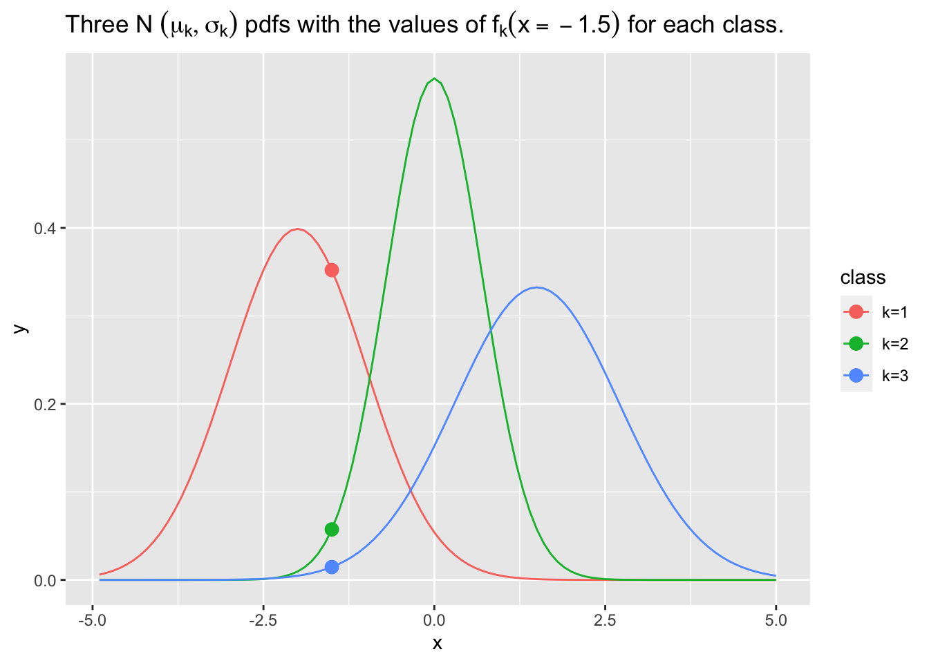
4.10.1 LDA/QDA Loss Function
A Loss Function describes the “cost” of an erroneous prediction; say we predict level (or class) \(\hat{y} =j\), when the actual level is \(y = k\) for some \(k\) and \(j\) out of the \(m\) categories.
\[ L(k|j) = \text{Loss from predicting } k\,| \text{ true class is }j. \tag{4.22}\]
We can define the risk of that loss as a function of the size of the loss \(\times\) the probability of that loss.
\[ \text{Risk}(\hat{y} = k |X) = (\text{Loss from predicting } k\,| X)p(k|X) = \sum_{j\neq k}^m L(k|j)p(j|X) \tag{4.23}\]
Our goal is to minimize Equation 4.23, i.e., to minimize our risk.
- We can view this in terms of minimizing the sum of weighted probabilities where the weights are the loss for each mis-classification, and, the probability is the posterior probability for the mis-classification given the \(X\) based on Equation 4.20.
4.10.2 The LDA/QDA Discriminant Function
Given we have \(m\) levels or classes of \(Y\), LDA and QDA will create \(m\) regions in the \(X\) space.
- If a new point \(x\) is in the region for level \(k\), will we predict \(\hat{y} = k\) for that \(x\).
LDA and QDA use a Discriminant Function to determine the boundaries (borders) between the \(m\) regions in the \(X\) space.
To create a discriminant function, let’s define a simple loss function as:
\[ L(\text{predict }k|\text{true class } j) = \cases {1 \text{ if } k \neq j \\ 0 \text{ if } k = j } \tag{4.24}\]
- This is known as a “Zero-One Loss”.
We can use Equation 4.24 to simplify Equation 4.23 as follows since all the \(L(k|j)=1\):
\[ \text{Minimize }\text{Risk}(\hat{y} = k |X) = \sum_{j\neq k} p(j|x) \]
Minimizing \(\sum_{j\neq k} p(j|x)\) is equivalent to maximizing its complement, or,
\[ \text{Maximum }p(k |X) = 1-\text{ Minimum}\sum_{j\neq k} p(j|X) \]
As a statistical machine learning method, we can quantitatively evaluate our performance so we can find a maximum.
We will compare the posterior probability \(p(k|X)\) with other possibilities, e.g., the posterior probability \(p(j|X)\), for all \((m-1)\) classes \(j \neq k\).
- This is just like KNN where we used the largest probability across the set of neighbors.
We can use Equation 4.20 and Equation 4.21 to compare the posterior probabilities of the two possible classes \(k\) and \(j.\)
- We would predict \(\hat{y} = k\) if \(p(k |x)\geq p(j |x)\) in the following:
\[ \begin{align} p(k |x) &= \frac{p(k)f_k(x)}{p(x)} = \frac{p(k)\frac{1}{\sigma_k\sqrt{2 \pi}} e^{\frac{-(x - \mu_k)^2}{2\sigma_k^2}}}{p(x)} \\ p(j|x) &= \frac{p(j)f_j(x)}{p(x)} = \frac{p(j)\frac{1}{\sigma_j\sqrt{2 \pi}} e^{\frac{-(x - \mu_j)^2}{2\sigma_j^2}}}{p(x)} \end{align} \tag{4.25}\]
When just comparing two potential levels \(k\) and \(j\) for a given set of \(x\), we can simplify Equation 4.25 thorough cancellation of common denominators \(\sqrt{2\pi}\) and \(p(x)\).
- We will predict \(\hat{y}=k\) if the quantity on the left side below is larger than the one on the right:
\[ p(k)\,\frac{1}{\sigma_k} e^{\frac{-(x - \mu_k)^2}{2\sigma_k^2}} > p(j)\,\frac{1}{\sigma_j} e^{\frac{-(x - \mu_j)^2}{2\sigma_j^2}} \tag{4.26}\]
Equation 4.26 is known as the Discriminant Function for comparing two levels.
The left side and right are no longer posterior probabilities. They are calculated based on the formulas Equation 4.26 such that if the left is larger than the right, then the posteriors have the same relationship i.e., \(p(y=k|x) > p(y=j|x).\)
- With two levels, \(k\) and \(j\), we would have two regions in \(x\) space. We define the boundary between them as the set of points where \(p(k|x) = p(j|x)\).
- If we have multiple levels or classes, we would have versions of Equation 4.26 for each pair and we define the boundaries based on where the posterior probabilities are equal.
- Since the probability of having an exact equality in Equation 4.26 for a given \(X\) is 0 (it’s a continuous probability distribution), we expect all points to fall on one side of the boundary or the other, so there are no ties.
- We have only one possible prediction for \(\hat{y}_i|x_i\).
A Bayesian way to think about Equation 4.26 is:
- We start with the prior probability that each class \(k\) or \(j\) is true.
- We then apply weights to get the posterior probabilities for whether \(k\) is true or \(j\) is true.
- The weights are based on the information we can get from the \(x\), namely the probability we would have gotten the \(x\) values we did if \(k\) were true or if \(j\) were true.
- If the \(k\) were true, we would expect \(p(x|k) > p(x | j)\) so the posterior probability of \(pk|x\) would be increased relatively more than \(p(j|x)\).
- Whether the posterior probability \(p(k|x) > p(j|x)\) depends then upon the relative starting values for the prior probabilities.
4.10.3 Example of Using the LDQ/QDA Discriminant Function
A quality inspector has to decide whether to accept or to reject a large shipment of parts based on a sample of 100 parts.
- The manufacturer claims only 3 out of 100 of the parts are defective on average with a variance of 2.5.
- Based on her years of examining samples from this manufacturer, the inspector believes she gets good samples 90% of the time.
- However, she also believes 10% of the time she can gets a bad sample where she expects 10 parts out of 100 to be defective with a variance of 9.
- She finds 7 defective parts in the sample.
Is this a good shipment or a bad shipment?
We want to classify the shipment as good or bad. Let’s match the data to each class
- Prior Probabilities:
- Good: Prior probability of good is 0.9. We don’t need the information from the sample to get this.
- Bad: Prior Probability of bad is 0.1. We don’t need the information from the sample to get this.
- Distributions of Good and Bad given an \(x.\)
- Good is Normal\((\mu = 3, \sigma^2 = 2.5)\)
- Bad is Normal\((\mu = 10, \sigma^2 = 9)\)
- \(x=.07\) given she got 7/100 as bad.
We now have all the information we need to compute and compare Posterior Probabilities using Equation 4.26.
\[ \begin{align} \text{Predict Good when}&\\ &\Downarrow\\ p(\text{Good})\frac{1}{\sigma_\text{Good}}e^{\frac{-(x-\mu_\text{Good})^2}{2\sigma^2_\text{Good}}} & \quad > \quad p(\text{Bad})\frac{1}{\sigma_\text{Bad}}e^{\frac{-(x-\mu_\text{Bad})^2}{2\sigma^2_\text{Bad}}}\\ &\Downarrow\\ .9 (\frac{1}{\sqrt{2.5}})e^{\frac{-(7-3)^2}{2(2.5)}} &\quad > \quad .1 (\frac{1}{\sqrt{9}})e^{\frac{-(7-10)^2}{2(9)}} \\ &\Downarrow\\ 0.023 &\quad > \quad 0.020 \end{align} \]
What happens if we play with the number of bad parts in the sample, \(x\), or the priors?
x <- 7
prior_good <- .9
prior_bad <- 1 - prior_good
good <- prior_good * (1/sqrt(2.5)) * exp(-(x - 3)^2 / (2 * 2.5))
round(good, 3)
[1] 0.023[1] 0.02[1] TRUEIf we want to calculate the actual posteriors, since we don’t know \(p(x)=p(\text{Good and Bad})\) directly, we can use Equation 4.20 and also use the denominator in Equation 4.19 (where Bad is the complement of Good or \(\text{Good}'\)) to get \(p(x)\).
- For \(p(\text{Sample is Good}| 7)\)
\[ \begin{align} p(\text{Good}| 7) & = \frac{ p(\text{Good})\frac{1}{\sigma_\text{Good}\sqrt{2\pi}}e^{\frac{-(7-\mu_\text{Good})^2}{2\sigma^2_\text{Good}}}}{p(\text{Good})\frac{1}{\sigma_\text{Good}\sqrt{2\pi}}e^{\frac{-(7-\mu_\text{Good})^2}{2\sigma^2_\text{Good}}} + p(\text{Bad})\frac{1}{\sigma_\text{Bad}\sqrt{2\pi}}e^{\frac{-(7-\mu_\text{Bad})^2}{2\sigma^2_\text{Bad}}} } \\ &\Downarrow\\ &= \frac{.9\frac{1}{\sqrt{2.5} \sqrt{2\pi}}e^{\frac{-(7-3)^2}{2(2.5)}}}{.9\frac{1}{\sqrt{2.5} \sqrt{2\pi}}e^{\frac{-(7-3)^2}{2(2.5)}} + .1\frac{1}{\sqrt{9} \sqrt{2\pi}}e^{\frac{-(7-10)^2}{2(9)}}}\\ &\Downarrow\\ &= \frac{0.05815942}{0.05815942+ 0.05067823} \\ &\Downarrow\\ p(\text{Good}| 7) &=0.534 \end{align} \]
Again, one can play with the priors or \(X\) to see how the posterior probability changes
4.10.4 The Log of the Discriminant Function
Since the log function is monotonic,(entirely non-decreasing or non-increasing) we can take the log of both sides of Equation 4.26 and the results of the maximization comparison will be in the same order (the log preserves the order of the transformed values).
Taking the log of \(p(k |X) > p(j |X)\) and choosing the larger value means we get the same predictions by making comparisons using the following:
\[ \begin{align} \text{Predict }\hat{y} = k \text{ when}& \\ \Downarrow&\\ \ln(p_k) -\ln(\sigma_k) -\frac{(x - \mu_k)^2}{2\sigma_k^2}\quad & >\quad \ln(p_j) -\ln(\sigma_j) -\frac{(x - \mu_j)^2}{2\sigma_j^2} \end{align} \tag{4.27}\]
Otherwise, predict \(\hat{y}|x = j\).
Equation 4.27 can make it easier to see all of the values in the formulas are constants except the \(x\).
- It can also be easier to compute at times.
4.10.5 The LDA Discriminant Function Assumes Equal Variance for All Classes
For LDA, we make an assumption to simplify Equation 4.27.
We assume \(\sigma_k = \sigma \, \forall\, k\); or homoscedasticity.
Having equal variances means we can can simplify Equation 4.27 by removing the subscripts on the \(\sigma^2.\)
This means Figure 4.5 now looks like the following:
Show code
x <- (seq(1:100) / 10) - 5
y1 <- dnorm(x, mean = -2 , sd = 1)
y2 <- dnorm(x, mean = 0, sd = 1)
y3 <- dnorm(x, mean = 1.5, sd = 1)
df <- tibble(class = c(rep("k=1", 100), rep("k=2", 100), rep("k=3", 100)),
                       x = c(x, x , x),
                       y = c(y1, y2, y3) )
ggplot(df, aes(x = x, y = y, color = class)) +
  geom_line() +
  geom_point(data = tibble(x1 = c(-1.5, -1.5, -1.5),
                           y1 = c(dnorm(-1.5, mean = -2 , sd = 1),
                                 dnorm(-1.5, mean = 0 , sd = 1),
                                 dnorm(-1.5, mean = 1.5 , sd = 1)),
                           class1 = c("k=1", "k=2", "k=3")),
             mapping = aes(x1, y1, color = class1), size = 3) +
  ggtitle(latex2exp::TeX("Three N $(\\mu_k, \\sigma)$ pdfs with the values of $f_k(x=-1.5)$ for each class."))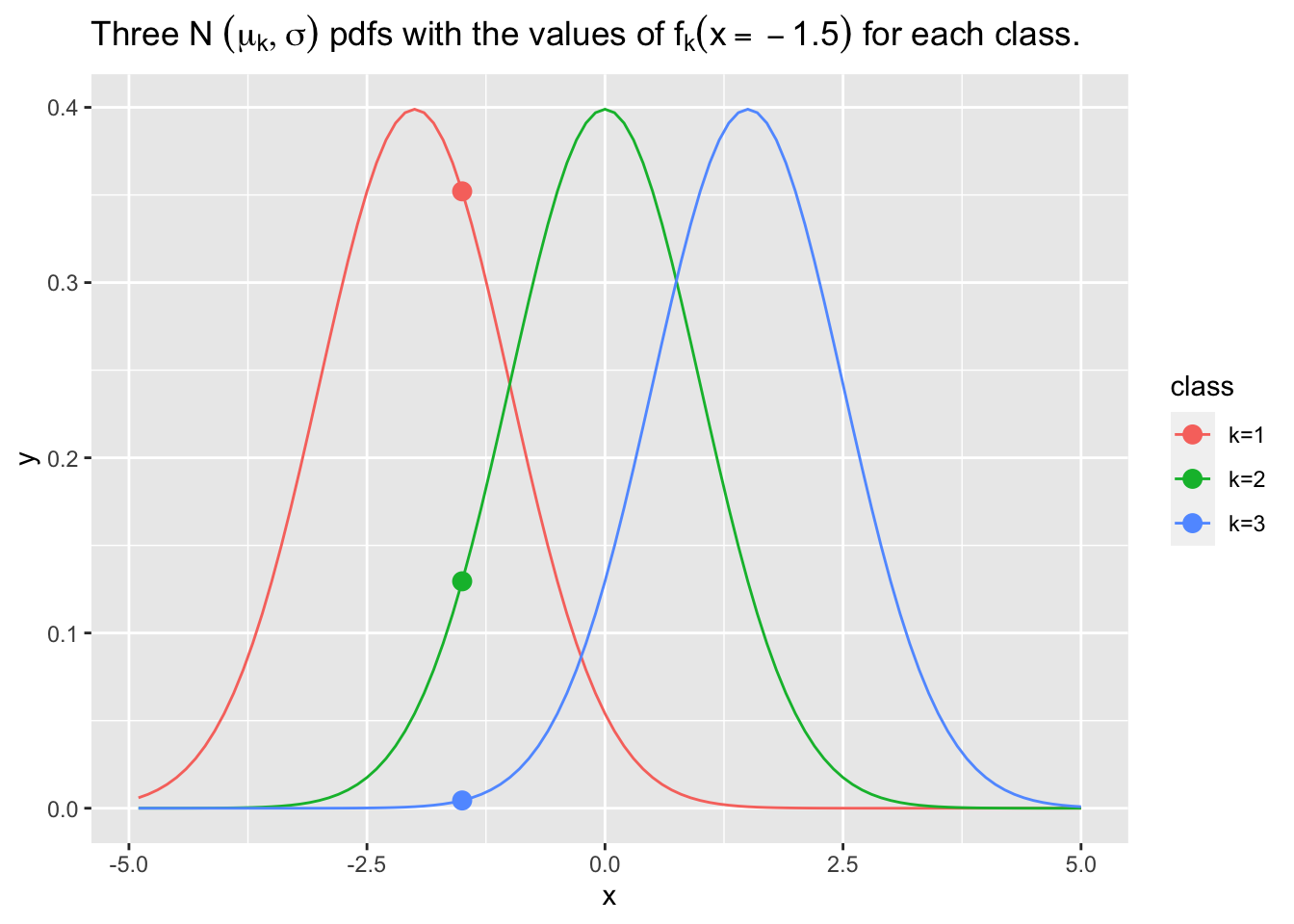
Figure 4.6 shows \(p(y=1|x) \geq p(y=2|x) >p(y=3|x).\) This means the prior for \(p(k=1)\) will be more heavily weighted than the others, increasing the likelihood of predicting \(y=1\).
Given the equal variances, let’s remove the subscripts on the \(\sigma\) and cancel out the \(\ln(\sigma)\) on both sides.
\[ \begin{align} \text{Predict }\hat{y} &= k \text{ when} &\\ \Downarrow&\\ \ln(p_k) -\frac{(x - \mu_k)^2}{2\sigma^2}\quad &>\quad \ln(p_j) -\frac{(x - \mu_j)^2}{2\sigma^2} \end{align} \tag{4.28}\]
Now multiply out the squared term \((x - \mu_k)^2\) (the squared difference between \(X\) and \(\mu_k\)) and move the minus sign across parentheses to remove them:
\[ \ln(p_k) -\frac{x^2}{2\sigma^2} + \frac{x\mu_k}{\sigma^2} - \frac{\mu_k^2}{2\sigma^2} > \ln(p_j) -\frac{x^2}{2\sigma^2} + \frac{x\mu_j}{\sigma^2} - \frac{\mu_j^2}{2\sigma^2} \]
Then, cancel the quadratic term \(\frac{x^2}{2\sigma^2}\) from both sides.
This creates the LDA Discriminant Function for comparing two regions:
\[ \begin{align} \text{Predict }\hat{y} &= k \text{ when} \\ &\Downarrow\\ \ln(p_k) +\frac{x\mu_k}{\sigma^2} - \frac{\mu_k^2}{2\sigma^2}&> \ln(p_j) + \frac{x\mu_j}{\sigma^2} - \frac{\mu_j^2}{2\sigma^2} \\ &\Downarrow\\ \text{Rearranging}&\text{ terms yields} \\ &\Downarrow\\ \ln(p_k) - \frac{\mu_k^2}{2\sigma^2} +\frac{\mu_k}{\sigma^2}x &> \ln(p_j) - \frac{\mu_j^2}{2\sigma^2} + \frac{\mu_j}{\sigma^2}x \end{align} \tag{4.29}\]
Losing the quadratic term \(\frac{x^2}{2\sigma^2}\) is what makes this Linear discriminant analysis as the function is now linear in the \(x\).
As a result the boundaries are straight lines.
In LDA, the boundaries are always linear.
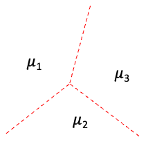
4.10.6 The QDA Discriminant Function
We stay with the original discriminant function and do not assume all the \(\sigma_k = \sigma\).
This means the quadratic terms in Equation 4.29 do not drop out, so you can have non-linear boundaries between regions as seen in Figure 4.7.
QDA tends to require more data for good performance compared to LDA since it using more degrees of freedom to estimate all the quadratic terms, especially for multiple predictors \(x\).
We use the original Equation 4.26 to determine the \(m\) class regions in \(X\) space.
The boundaries are where the comparisons in Equation 4.26 (or the posterior probabilities) are equal.
Like LDA, the probability of an \(x\) being exactly on the nonlinear boundary is 0 so we can use \(\geq\) or \(>\) in the comparison.
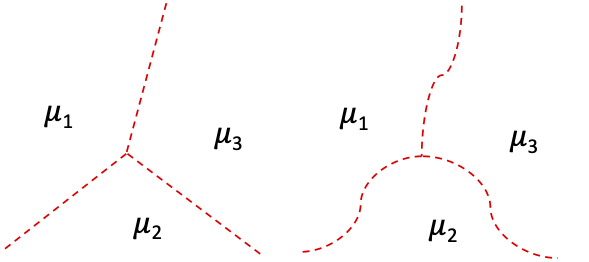
4.10.7 Multiple \(X\)
When we have multiple predictors in \(\bf{X}\), there are multiple \(f_{k,i}(x)\) each of which has its own \(\mu_{k,i}\).
The points where the inequality becomes an equality in Equation 4.29 are still the discriminant boundary between two classes (aka the decision boundary).
Given discriminant boundaries for three classes, we would estimate
\(\hat{y} = 1\) if \(p(1|\bf{X})\) is the largest
\(\hat{y} = 2\) if \(p(2|\bf{X})\) is the largest
\(\hat{y} = 3\) if \(p(3|\bf{X})\) is the largest
- Whichever posterior probability for a class is highest, that class \(k\) is our prediction.
- It is based on the relative values of the prior probabilities and the weights from the \(p(k|\bf{X})\).
4.10.8 No Prior Preference Across Classes
If we have no prior information as to which class has the highest probability, then our prior can be \(p(k) = 1/m\) (where \(m = \text{number of classes}\)) which is a constant.
- For three classes, \(p(k) = 1/3\).
That means \(\ln(p(k)) = \ln(p(m))\) in Equation 4.29.
- Thus, we can simplify Equation 4.27 (in a different way than before) by dropping off the log of the priors, \(\ln(p(k))\), to get:
\[ \begin{align} \text{Predict }\hat{y} = k &\text{ when} \\ \Downarrow&\\ \ln(p_k) -\ln(\sigma_k) -\frac{(x - \mu_k)^2}{2\sigma_k^2}& \quad > \quad \ln(p_j) -\ln(\sigma_j) -\frac{(x - \mu_j)^2}{2\sigma_j^2} \\ \Downarrow&\\ -\ln(\sigma_k) -\frac{(x - \mu_k)^2}{2\sigma_k^2}& \quad > \quad -\ln(\sigma_j) -\frac{(x - \mu_j)^2}{2\sigma_j^2} \end{align} \tag{4.30}\]
And if we also assume \(\sigma_k = \sigma\) (so we are using LDA), Equation 4.30 becomes
\[ \begin{align} -\frac{(x - \mu_k)^2}{2\sigma^2} &> -\frac{(x - \mu_j)^2}{2\sigma^2}.\\ \\ \text{Cancel the }& 2 \sigma^2 \text{ to get}\\ \\ \text{Predict }&\hat{y} = k \text{ when} \\ \Downarrow&\\ - (x - \mu_k)^2 & > -(x - \mu_j)^2 \end{align} \tag{4.31}\]
Maximizing the left side of Equation 4.31 is equivalent to minimizing the left side of the following over the choice of \(k\).
\[ \begin{align} \text{Predict }\hat{y} &= k \text{ when} \\ \Downarrow&\\ (x - \mu_k)^2 &< (x - \mu_j)^2 \end{align} \tag{4.32}\]
This means we are classifying \(\hat{y}_i=k\) when \(x_i\) is closest to \(\mu_k\) or \(\hat{y}|x =k_{x_i\text{ closest to }\mu_k}\).
Given a point \(x\) to predict, if you have the same priors, you do not have to do all the computations, you just find the \(\mu_k\) which is closest to \(x\) based on Euclidean distance.
If you have distinct prior probabilities, the boundaries will be shifted away from the \(\mu_k\) with the larger priors, and your prediction (after all the calculations) may not be the closest \(\mu_k\).
4.10.9 LDA/QDA Example in R with Home Sales Data
Let’s use the HOME SALES.csv data. You can download/read the data from https://raw.githubusercontent.com/rressler/data_raw_courses/main/HOME_SALES.csv.
suppressMessages(library(tidyverse))
home <- read_csv("https://raw.githubusercontent.com/rressler/data_raw_courses/main/HOME_SALES.csv")
glimpse(home)
Rows: 522
Columns: 13
$ ID <dbl> 1, 2, 3, 4, 5, 6, 7, 8, 9, 10, 11, 12, 13, 14, 15, 16,…
$ SALES_PRICE <dbl> 360000, 340000, 250000, 205500, 275500, 248000, 229900…
$ FINISHED_AREA <dbl> 3032, 2058, 1780, 1638, 2196, 1966, 2216, 1597, 1622, …
$ BEDROOMS <dbl> 4, 4, 4, 4, 4, 4, 3, 2, 3, 3, 7, 3, 5, 5, 3, 5, 2, 3, …
$ BATHROOMS <dbl> 4, 2, 3, 2, 3, 3, 2, 1, 2, 3, 5, 4, 4, 4, 3, 5, 2, 4, …
$ GARAGE_SIZE <dbl> 2, 2, 2, 2, 2, 5, 2, 1, 2, 1, 2, 3, 3, 2, 2, 2, 2, 2, …
$ YEAR_BUILT <dbl> 1972, 1976, 1980, 1963, 1968, 1972, 1972, 1955, 1975, …
$ STYLE <dbl> 1, 1, 1, 1, 7, 1, 7, 1, 1, 1, 7, 1, 7, 5, 1, 6, 1, 7, …
$ LOT_SIZE <dbl> 22221, 22912, 21345, 17342, 21786, 18902, 18639, 22112…
$ AIR_CONDITIONER <chr> "YES", "YES", "YES", "YES", "YES", "YES", "YES", "YES"…
$ POOL <chr> "NO", "NO", "NO", "NO", "NO", "YES", "NO", "NO", "NO",…
$ QUALITY <chr> "MEDIUM", "MEDIUM", "MEDIUM", "MEDIUM", "MEDIUM", "MED…
$ HIGHWAY <chr> "NO", "NO", "NO", "NO", "NO", "NO", "NO", "NO", "NO", …We will use the LDA functions in the {MASS} package (Modern Applied Statistics in S).
- Use the console to install the package and then load it with
library(MASS).
We can see Quality is character and has three levels.
Let’s use LDA to predict QUALITY based on SALES_PRICE and YEAR_BUILT and see how we do.
We can use GGally::ggpairs() to plot our three variables of interest.
With two predictors, we can also plot as a scatter plot and code by color
Show code

Do these look look like we should use Linear or Non-Linear boundaries?
Let’s try LDA first.
Call:
lda(QUALITY ~ SALES_PRICE + YEAR_BUILT, data = home)

Prior probabilities of groups:
     HIGH       LOW    MEDIUM
0.1302682 0.3141762 0.5555556

Group means:
       SALES_PRICE YEAR_BUILT
HIGH      543610.6   1986.029
LOW       175018.3   1952.640
MEDIUM    273766.3   1970.486

Coefficients of linear discriminants:
                      LD1           LD2
SALES_PRICE -1.095489e-05 -6.415934e-06
YEAR_BUILT  -2.302181e-02  6.995451e-02

Proportion of trace:
   LD1    LD2
0.9568 0.0432 - We don’t know the true means \(\mu_{k,i}\) for our two predictors, so
lda()used sample means for each subset to estimate the Group means. - The Coefficients of linear discriminant are the linear combination of the predictor variables that create the decision boundaries based on scaling the data to have equal variances.
- The Proportion of trace is the percentages of the separation achieved by each linear discriminant function.
We do not have to separate training and testing as we can set the CV=argument to TRUE and LDA() will conduct cross-validation for us. (We will discuss cross-validation in more detail later on in the course.)
LDA_result <-  lda(QUALITY ~ SALES_PRICE + YEAR_BUILT, CV = TRUE, data = home)
LDA_result$class[1:15]
[1] MEDIUM MEDIUM MEDIUM MEDIUM MEDIUM MEDIUM MEDIUM LOW MEDIUM LOW
[11] MEDIUM HIGH HIGH HIGH MEDIUM
Levels: HIGH LOW MEDIUM [1] 2.516926e-02 1.290005e-02 3.728255e-04 2.411230e-05 6.662849e-04
[6] 2.474351e-04 1.143724e-04 9.267011e-07 2.968788e-05 4.049867e-08
[11] 1.456840e-05 9.935778e-01 9.810900e-01 9.618354e-01 3.713793e-03Note: the posterior results are just first 15 elements in the first column of the posterior matrix in the LDA object.
It gives a different result in that it produces all of the predictions and the posterior probabilities that is used to make the predictions for every house!
Let’s look at a sample of these:
            HIGH          LOW       MEDIUM LDA_result.class
317 8.603264e-05 1.331705e-01 0.8667434239           MEDIUM
151 8.703173e-01 1.996681e-04 0.1294829825             HIGH
242 1.504830e-04 6.724846e-02 0.9326010557           MEDIUM
385 1.716326e-06 7.303381e-01 0.2696601951              LOW
381 4.413334e-06 6.038325e-01 0.3961630454              LOW
178 2.871680e-01 5.203293e-03 0.7076286915           MEDIUM
414 1.591111e-05 3.308850e-01 0.6690990899           MEDIUM
152 1.298639e-01 7.525748e-03 0.8626103755           MEDIUM
87  9.997281e-01 7.036161e-08 0.0002718482             HIGH
203 9.249500e-01 1.629424e-03 0.0734205920             HIGH
We can see the posterior probabilities for each region and that the category with the largest one is how it predicted.
Let’s plot the results.
plot_home
# create data frame with classifications and true values
lda_df <- tibble(price = home$SALES_PRICE, year = home$YEAR_BUILT,
                 class = LDA_result$class) |>
  rownames_to_column(var = "ID") |>
  arrange(as.numeric(ID)) |>
  bind_cols(true_q = home$QUALITY)

ggplot(lda_df, aes(price, year, color = class)) +
  geom_point(alpha = .5, size = .5) ->
  plot_class
plot_class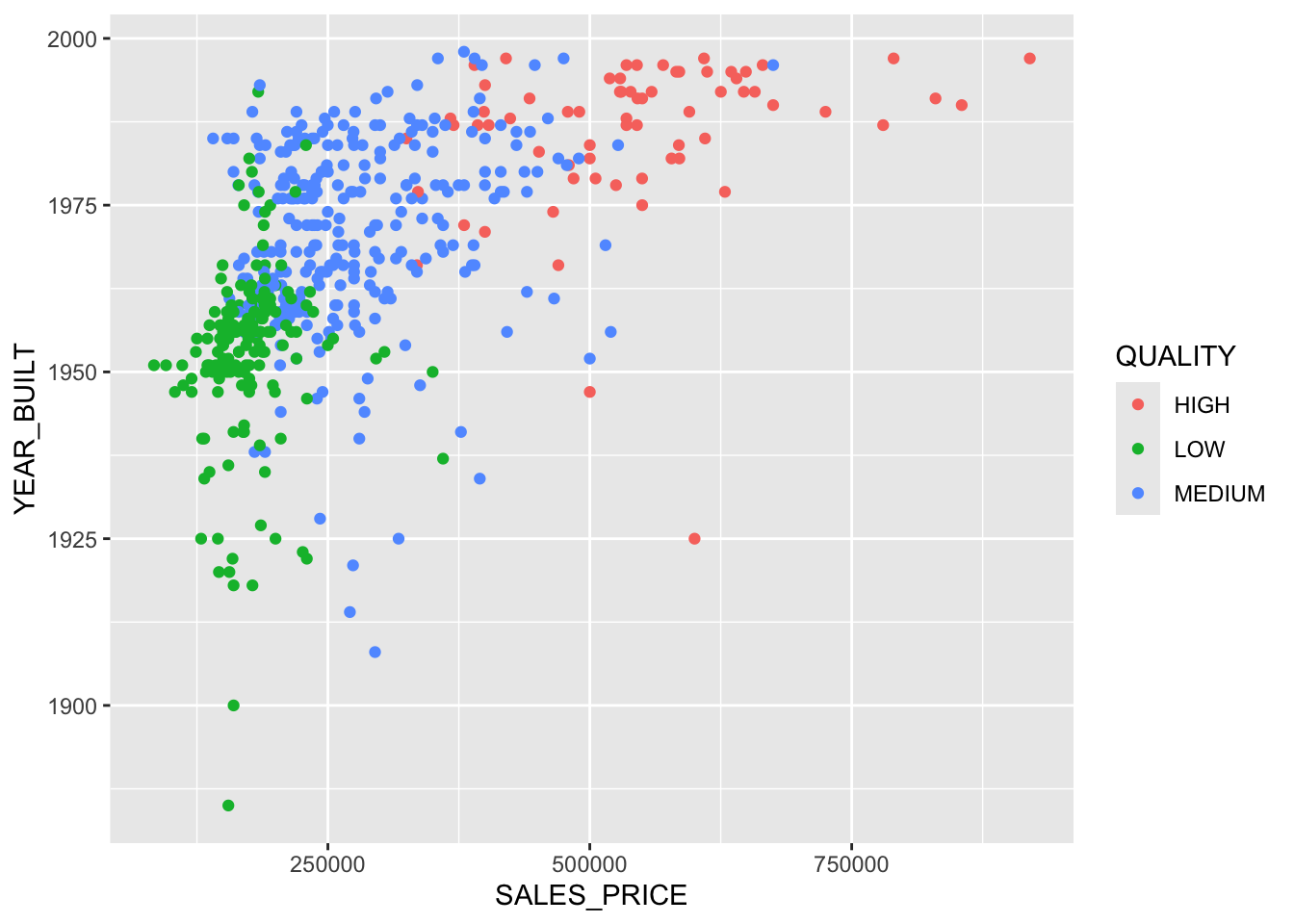

We can see that we have linear boundaries now.
Let’s look at the classification errors.
Show code

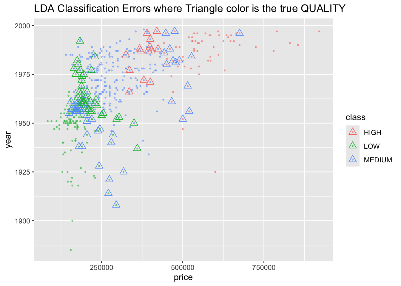
So while we have linear boundaries, there are errors.
Let’s try QDA now using MASS::qda() with CV = TRUE.
Show code
 [1] MEDIUM MEDIUM MEDIUM LOW    MEDIUM MEDIUM MEDIUM LOW    MEDIUM LOW
[11] LOW    HIGH   HIGH   HIGH   MEDIUM
Levels: HIGH LOW MEDIUM [1] 7.111682e-02 5.926188e-02 1.536402e-02 1.371178e-03 1.083137e-02
[6] 8.934994e-03 6.265528e-03 1.613207e-04 4.101128e-03 4.399966e-08
[11] 1.416419e-03 9.829055e-01 9.581961e-01 9.223142e-01 4.497300e-02plot_home
# create data frame with classifications and true values
qda_df <- tibble(price = home$SALES_PRICE, year = home$YEAR_BUILT,
class = QDA_result$class) |>
rownames_to_column(var = "ID") |>
arrange(as.numeric(ID)) |>
bind_cols(true_q = home$QUALITY)
ggplot(qda_df, aes(price, year, color = class)) +
geom_point(alpha = .5) ->
plot_classq
plot_classq
plot_classq +
geom_point(data = qda_df[qda_df$class != qda_df$true_q,],
mapping = aes(price, year, color = true_q), shape = 2, size = 3) +
ggtitle("QDA Classification Errors where Triangle color is the true QUALITY")
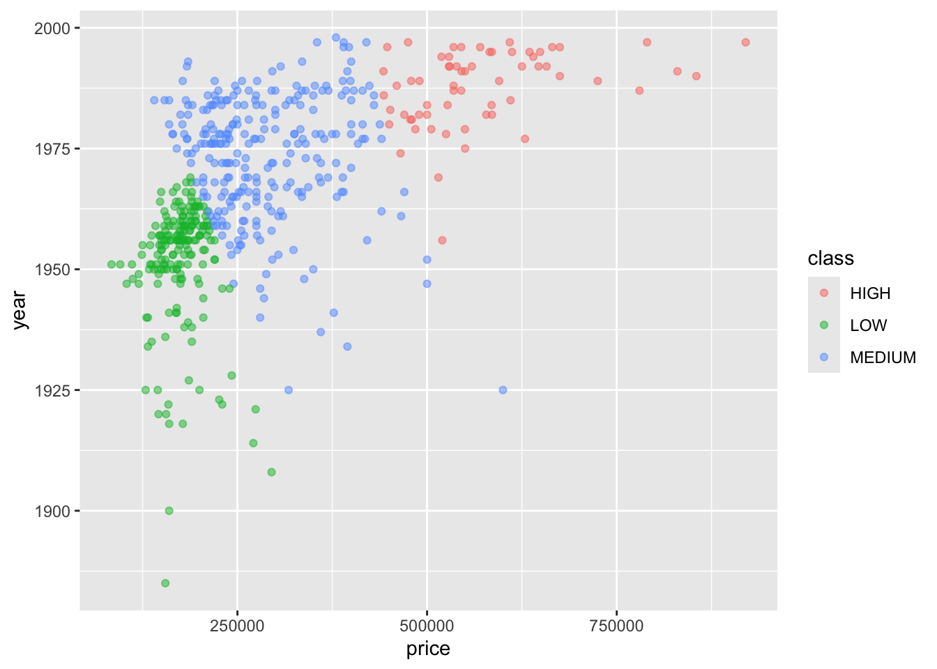
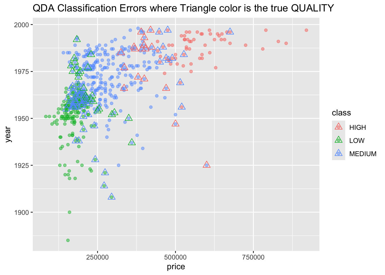
[1] 19.35[1] 20.88What does it mean that LDA did better than QDA?
4.11 General Linear Models (Chap 4.6)
4.11.1 Poisson Regression
We have looked at predicting a quantitative response variable using regression and predicting a categorical response variable with a few levels using KNN, Logistic Regression, and LDA/QDA.
What about a response variable that can take on many values, but they have to be whole numbers \(\{0, 1, 2, 3, \ldots\}\)?
Count Data covers cases where a response variable \(Y \geq 0\) and \(Y \in \mathbb{W}\). (the Whole numbers)
One can do linear regression on count data, but you can run into the same issues we saw before with categorical data.
Predictions may be negative or non-integer so difficult to interpret.
The assumption of \(\text{Var}(\epsilon_i) = \sigma^2 \, \forall Y\) may not be appropriate, e.g., the variance may increase as \(Y\) increases.
Poisson Regression is an alternative to linear regression when the response variable is counts.
4.11.2 The Poisson Distribution
If a random variable \(Y\) takes on non-negative integer values representing events per unit time, it may be reasonable to model it using the Poisson Distribution.
Assumptions:
- The events occur at a constant average rate
- The time between events is independent of the time of the previous event (a memory-less process).
With these assumptions, the Poisson distribution has a distribution function with one parameter, \(\lambda\):
\[ P(Y = k) = \frac{e^{-\lambda} \lambda^k}{k!} \tag{4.33}\]
- where \(k\) is the number of events in a period of time (a count value) and
- \(\lambda = E[Y]\) is known as the rate parameter: the expected number of events in the period.
- Note that \(\text{Var}(Y) = \lambda\).
- This means that as the mean of \(Y\) increases, so does its variance.
The Poisson distribution is often used in modeling counts, such as in time series (hourly, daily, monthly totals) or queuing theory, how many customers arrive at the cash register line in a given period.
If the count of events follows the Poisson distribution with rate parameter \(\lambda\), the inter-arrival time of the events follows the exponential distribution, with the sample value of \(\lambda\).
4.11.3 Using the Poisson Distribution in Regression
We are interested in predicting the counts in a given period of time where the rate of events for that period may depend upon other covariates \(X\).
We can express mathematically where \(\lambda\) is a function of the \(X\) such as
\[ \lambda(X_1, X_2, \ldots, X_p) = e^{\beta_0 + \beta_1 X_1 + \beta_2 X_2 + \cdots + \beta_p X_p} \tag{4.34}\]
or, equivalently
\[ \ln\left(\lambda(X_1, X_2, \ldots, X_p)\right) = \beta_0 + \beta_1 X_1 + \beta_2 X_2 + \cdots + \beta_p X_p \tag{4.35}\]
Equation 4.35 may be referred to as log-linear regression.
We can use Equation 4.33 and Equation 4.34 to set up a Poisson regression model where \(\ln(\lambda)\) is linear in the \(X\) as before.
We can use the same maximum likelihood estimation procedure we used for Logistic Regression but with Equation 4.33 and Equation 4.35.
For a sample of \(n\) values of \((y_i, X_i)\), we will maximize the following likelihood \(\text{L}\) as function of the \(\beta_i\)s so the coefficients make the observed data as likely as possible:
\[ \text{L}(\beta_0, \beta_1, \beta_2, \ldots, \beta_p) = \prod_{1=1}^{n}\left(\frac{e^{-\lambda(x_i)}\lambda(x_i)^{y_i} }{y_i!}\right) \tag{4.36}\]
We can fit this model using the R glm() function with the argument family = poisson.
Using the bikeshare data from {ISLR2} we see:
Rows: 8,645
Columns: 15
$ season     <dbl> 1, 1, 1, 1, 1, 1, 1, 1, 1, 1, 1, 1, 1, 1, 1, 1, 1, 1, 1, 1,…
$ mnth       <fct> Jan, Jan, Jan, Jan, Jan, Jan, Jan, Jan, Jan, Jan, Jan, Jan,…
$ day        <dbl> 1, 1, 1, 1, 1, 1, 1, 1, 1, 1, 1, 1, 1, 1, 1, 1, 1, 1, 1, 1,…
$ hr         <fct> 0, 1, 2, 3, 4, 5, 6, 7, 8, 9, 10, 11, 12, 13, 14, 15, 16, 1…
$ holiday    <dbl> 0, 0, 0, 0, 0, 0, 0, 0, 0, 0, 0, 0, 0, 0, 0, 0, 0, 0, 0, 0,…
$ weekday    <dbl> 6, 6, 6, 6, 6, 6, 6, 6, 6, 6, 6, 6, 6, 6, 6, 6, 6, 6, 6, 6,…
$ workingday <dbl> 0, 0, 0, 0, 0, 0, 0, 0, 0, 0, 0, 0, 0, 0, 0, 0, 0, 0, 0, 0,…
$ weathersit <fct> clear, clear, clear, clear, clear, cloudy/misty, clear, cle…
$ temp       <dbl> 0.24, 0.22, 0.22, 0.24, 0.24, 0.24, 0.22, 0.20, 0.24, 0.32,…
$ atemp      <dbl> 0.2879, 0.2727, 0.2727, 0.2879, 0.2879, 0.2576, 0.2727, 0.2…
$ hum        <dbl> 0.81, 0.80, 0.80, 0.75, 0.75, 0.75, 0.80, 0.86, 0.75, 0.76,…
$ windspeed  <dbl> 0.0000, 0.0000, 0.0000, 0.0000, 0.0000, 0.0896, 0.0000, 0.0…
$ casual     <dbl> 3, 8, 5, 3, 0, 0, 2, 1, 1, 8, 12, 26, 29, 47, 35, 40, 41, 1…
$ registered <dbl> 13, 32, 27, 10, 1, 1, 0, 2, 7, 6, 24, 30, 55, 47, 71, 70, 5…
$ bikers     <dbl> 16, 40, 32, 13, 1, 1, 2, 3, 8, 14, 36, 56, 84, 94, 106, 110…
What do we notice from the following plots?
Show code
ggplot(Bikeshare, aes(x = hr, y = bikers)) +
  geom_boxplot(notch = TRUE)
ggplot(Bikeshare, aes(x = mnth, y = bikers)) +
  geom_boxplot(notch = TRUE)
ggplot(Bikeshare, aes(x = as.factor(workingday), y = bikers)) +
  geom_boxplot(notch = TRUE)
ggplot(Bikeshare, aes(x = as.factor(season), y = bikers)) +
  geom_boxplot(notch = TRUE)
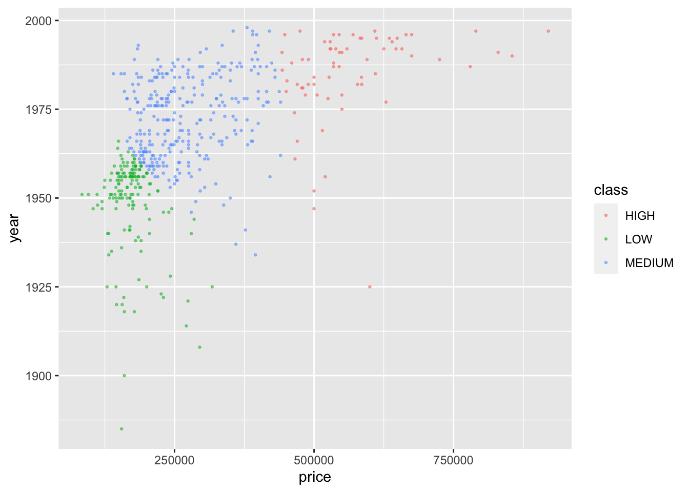
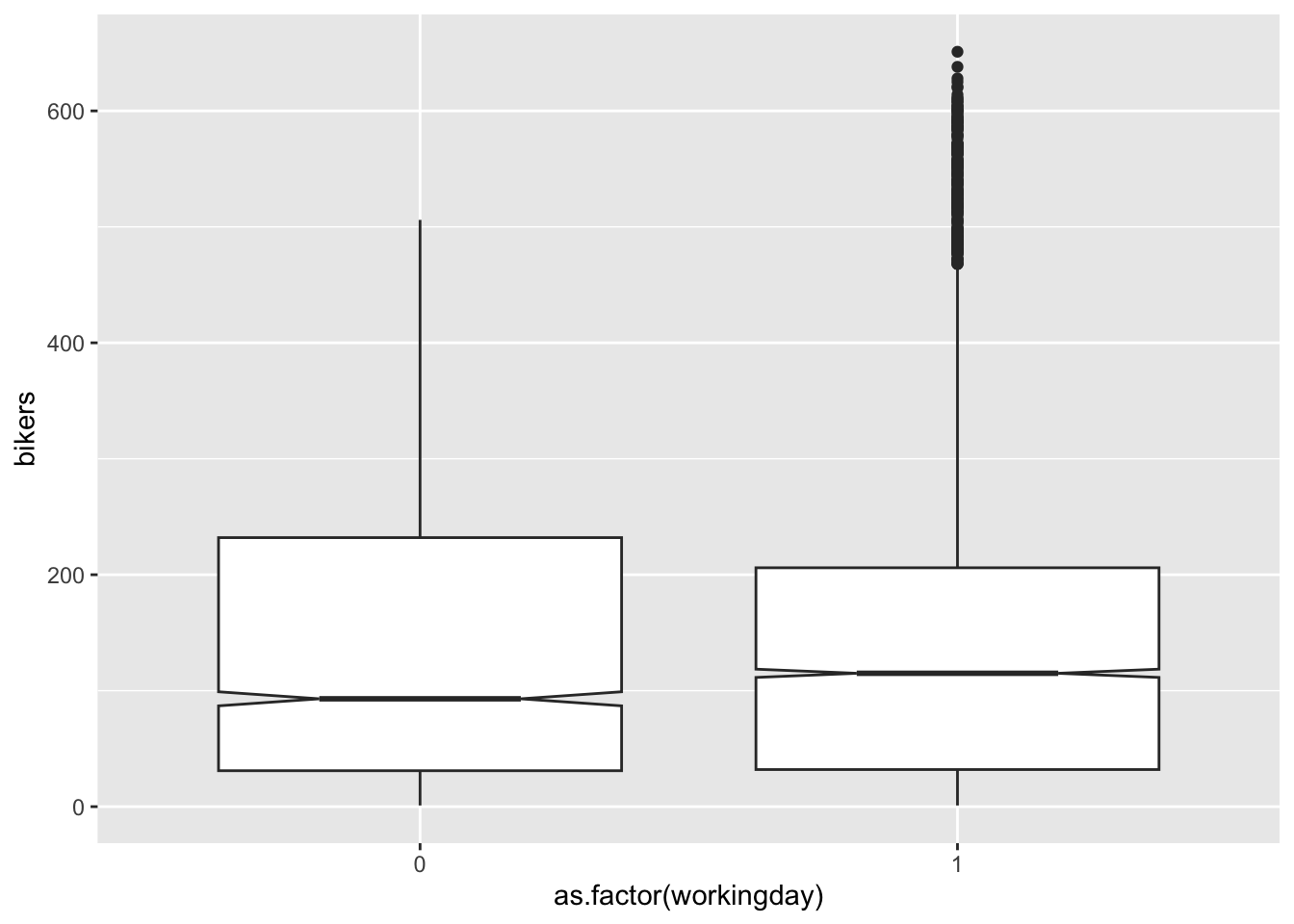
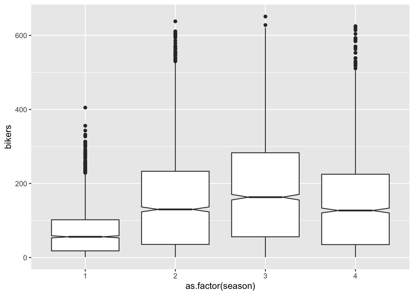
Let’s run the Poisson regression model in R with all the variables.
We see similar output from summary() with logistic regression.
- Variables have estimates and \(z\)-values which generate \(p\) values.
- Categorical Predictors have the first level built into \(\beta_0\).
- We see that R sets the dispersion parameter equal to 1 for Poisson regression.
- Some packages return an estimate of the dispersion so you can check the assumption \(E[Y] = \text{Var}(Y) = \lambda\).
- Let’s define a dispersion parameter \(\sigma^2\) as
\[ \sigma^2 = \frac{\text{Var}(y)}{\bar{y}} \]
- There are two cases:
- Over-dispersion is when Dispersion > 1 or the variance is greater than the mean.
- Under-dispersion is when Dispersion < 1 or the variance is less than the mean.
- We get Deviance for the Null model based on \(\bar{y}\) and for the fitted model as the Residual deviance
- Lower is better.
- We can perform a \(\chi^2\) goodness of fit in ANOVA where the Null hypothesis is none of the fitted model parameters are useful.
- Use the
anova()argumenttest = "Chisq".
Show code
Analysis of Deviance Table

Model 1: bikers ~ 1
Model 2: bikers ~ season + mnth + day + hr + holiday + weekday + workingday +
    weathersit + temp + atemp + hum + windspeed + casual + registered
  Resid. Df Resid. Dev Df Deviance  Pr(>Chi)
1      8644    1052921
2      8596      73349 48   979573 < 2.2e-16 ***
---
Signif. codes: 0 '***' 0.001 '**' 0.01 '*' 0.05 '.' 0.1 ' ' 1[1] NA 0[1] NA 0Let’s compare the full models to a reduced one without workingday using anova() with argument test = "Chisq".
Show code
Call:
glm(formula = bikers ~ ., family = poisson, data = Bikeshare[,
    -7])

Coefficients:
                            Estimate Std. Error z value Pr(>|z|)
(Intercept)                3.1332743  0.0111685 280.546  < 2e-16 ***
season                     0.0442355  0.0021270  20.797  < 2e-16 ***
mnthFeb                    0.1850230  0.0075896  24.379  < 2e-16 ***
mnthMarch                  0.2598251  0.0090228  28.797  < 2e-16 ***
mnthApril                  0.3485542  0.0116756  29.853  < 2e-16 ***
mnthMay                    0.3991351  0.0142909  27.929  < 2e-16 ***
mnthJune                   0.3685783  0.0173109  21.292  < 2e-16 ***
mnthJuly                   0.3511637  0.0203330  17.271  < 2e-16 ***
mnthAug                    0.3561679  0.0231060  15.414  < 2e-16 ***
mnthSept                   0.3930194  0.0260056  15.113  < 2e-16 ***
mnthOct                    0.3701511  0.0290438  12.745  < 2e-16 ***
mnthNov                    0.4026775  0.0320187  12.576  < 2e-16 ***
mnthDec                    0.4222760  0.0348912  12.103  < 2e-16 ***
day                       -0.0004293  0.0001035  -4.149 3.34e-05 ***
hr1                       -0.4088678  0.0130004 -31.450  < 2e-16 ***
hr2                       -0.7148055  0.0146485 -48.797  < 2e-16 ***
hr3                       -1.3128586  0.0188462 -69.662  < 2e-16 ***
hr4                       -1.9169856  0.0248001 -77.298  < 2e-16 ***
hr5                       -0.9513635  0.0160791 -59.168  < 2e-16 ***
hr6                        0.2418982  0.0106186  22.781  < 2e-16 ***
hr7                        0.7617542  0.0092622  82.243  < 2e-16 ***
hr8                        0.7902868  0.0093253  84.747  < 2e-16 ***
hr9                        0.8509716  0.0091246  93.261  < 2e-16 ***
hr10                       0.7138385  0.0093417  76.414  < 2e-16 ***
hr11                       0.7522563  0.0092389  81.422  < 2e-16 ***
hr12                       0.7896779  0.0091801  86.020  < 2e-16 ***
hr13                       0.7817365  0.0092281  84.713  < 2e-16 ***
hr14                       0.7649348  0.0092838  82.394  < 2e-16 ***
hr15                       0.7756958  0.0092662  83.712  < 2e-16 ***
hr16                       0.8279633  0.0091410  90.577  < 2e-16 ***
hr17                       0.6902508  0.0094616  72.953  < 2e-16 ***
hr18                       0.7276162  0.0093479  77.837  < 2e-16 ***
hr19                       0.8387727  0.0090601  92.579  < 2e-16 ***
hr20                       0.8170819  0.0091064  89.726  < 2e-16 ***
hr21                       0.7371047  0.0092738  79.482  < 2e-16 ***
hr22                       0.6202568  0.0095603  64.878  < 2e-16 ***
hr23                       0.3683042  0.0102115  36.067  < 2e-16 ***
holiday                   -0.0444951  0.0060308  -7.378 1.61e-13 ***
weekday                    0.0049529  0.0004563  10.854  < 2e-16 ***
weathersitcloudy/misty     0.0105555  0.0023158   4.558 5.16e-06 ***
weathersitlight rain/snow -0.1840704  0.0044635 -41.239  < 2e-16 ***
weathersitheavy rain/snow -0.5481551  0.1668317  -3.286  0.00102 **
temp                      -0.3373441  0.0405869  -8.312  < 2e-16 ***
atemp                      0.6189882  0.0431092  14.359  < 2e-16 ***
hum                       -0.0512983  0.0068469  -7.492 6.77e-14 ***
windspeed                 -0.0396834  0.0081116  -4.892 9.97e-07 ***
casual                     0.0040722  0.0000237 171.832  < 2e-16 ***
registered                 0.0037556  0.0000121 310.406  < 2e-16 ***
---
Signif. codes:  0 '***' 0.001 '**' 0.01 '*' 0.05 '.' 0.1 ' ' 1

(Dispersion parameter for poisson family taken to be 1)

    Null deviance: 1052921  on 8644  degrees of freedom
Residual deviance:   73351  on 8597  degrees of freedom
AIC: 126484

Number of Fisher Scoring iterations: 5Analysis of Deviance Table
Model 1: bikers ~ season + mnth + day + hr + holiday + weekday + weathersit +
temp + atemp + hum + windspeed + casual + registered
Model 2: bikers ~ season + mnth + day + hr + holiday + weekday + workingday +
weathersit + temp + atemp + hum + windspeed + casual + registered
Resid. Df Resid. Dev Df Deviance Pr(>Chi)
1 8597 73351
2 8596 73349 1 2.1054 0.1468[1] NA 0.1467773- We use the deviance tests with only nested models.
- We also check if the data violates some assumptions of the Poisson model that might suggest a more sophisticated approach (such as negative binomial).
- \(\bar{y} =\) 143.7944477
- \(\text{Var}(y) =\) 1.7901866^{4}
How to interpret the coefficients?
- An increase in \(X_j\) by one unit is associated with a change in \(E(Y) = \lambda\) by a factor of \(e^{\beta_j}\).
- We are estimating the expected value (the count) for a given period.
- As an expected value, it is likely not an integer.
We can predict with predict() and set the type = "response" to get the output in terms of the original \(\lambda\).
\[ \begin{align} \ln(\text{Expected number of Bikers per hour}) &= \beta_0 + \beta_{mtn}\text{mnth} + \beta_{hr}\text{hr} + \\ & \quad \beta_{workingday}\text{workingday} + \\ & \quad \beta_{temp}\text{temp} + \beta_{weathersit}\text{weathersit} + \\ & \quad \cdots \end{align} \]
       1        2        3        4        5        6
3.326104 3.006758 2.669924 2.005175 1.355113 2.309179 1 2 3 4 5 6
27.829714 20.221741 14.438867 7.427395 3.877201 10.066160 1 2 3 4 5 6
27.829714 20.221741 14.438867 7.427395 3.877201 10.066160 4.12 Generalized Linear Models
We have looked at three versions of the general linear model.
Each uses predictors \(X_1,\ldots,X_p\) to predict a response \(Y\).
Each assumes, that conditional on the \(X\), \(Y\) belongs to a specific family of distributions where we are trying to estimate the parameters of the distribution.
Each models the mean of \(Y\) as a function of the predictors \(X\).
- Linear Regression: Normal Distribution, \(E[Y|X] = \beta_0 + \beta_1 X_1 + \beta_2 X_2 + \cdots + \beta_p X_p\)
- Logistic Regression: Bernoulli Distribution \(E[Y|X] = \frac{e^{\beta_0 + \beta_1 X_1 + \beta_2 X_2 + \cdots + \beta_p X_p}}{1 + e^{\beta_0 + \beta_1 X_1 + \beta_2 X_2 + \cdots + \beta_p X_p}}\)
- Poisson Regression: Poisson Distribution: \(E[Y|X] = e^{\beta_0 + \beta_1 X_1 + \beta_2 X_2 + \cdots + \beta_p X_p}\)
We can transform the left side of each of so the formula is linear in predictors and then “generalize” them using a link function \(\eta\) (eta).
\[ \eta(E[Y|X]) = \beta_0 + \beta_1 X_1 + \beta_2 X_2 + \cdots + \beta_p X_p \]
where:
- Linear Regression: \(\eta(\mu) = \mu\)
- Logistic Regression: \(\eta(\mu) = \ln\left(\frac{1-\mu}{\mu}\right)\)
- Poisson Regression: \(\eta(\mu) = \ln(\mu)\)
The Normal, Bernoulli, and Poisson distributions are all members of a wider class of distributions, known as the Exponential family.
- Other members include the Exponential distribution, the Gamma distribution, and the Negative Binomial distribution.
- See help for
familyin {stats}. - Each of these distributions may be useful in modeling certain phenomena.
A regression approach that performs a regression by using a “link function” to model the response \(Y\) as a member of the broad exponential family, and then transforming the expected value of \(Y\) to be a linear function of the predictors, can be termed a Generalized Linear Model (GLM).
