9 Support Vector Machine Methods
9.1 Support Vector Machines
We saw that trees split the \(\bf{X}\) space by using binary trees which can be restrictive.
Support Vector Machine (SVM) methods take the binary tree concept but split the \(\bf{X}\) space geometrically to provide more flexibility.
SVM methods are for classification and regression. We will cover classification.
The goal: Find the best split of the \(\bf{X}\)-space with the given form of boundaries to make the best prediction of a categorical response \(Y\).
Forms can be linear, polynomial, radial, or sigmoid.
- Linear: splits based on lines. Find the best lines that separates the \(Y\).
- Polynomial: splits based on curves. Find the best curves that separates the \(Y\).
- Radial: splits based on circles/spheres.
- Sigmoid: splits based on a sigmoid (S-shaped) function such as we used in logistic regression.
We will start with the simplest SVM methods
9.2 Maximal Margin Classifier
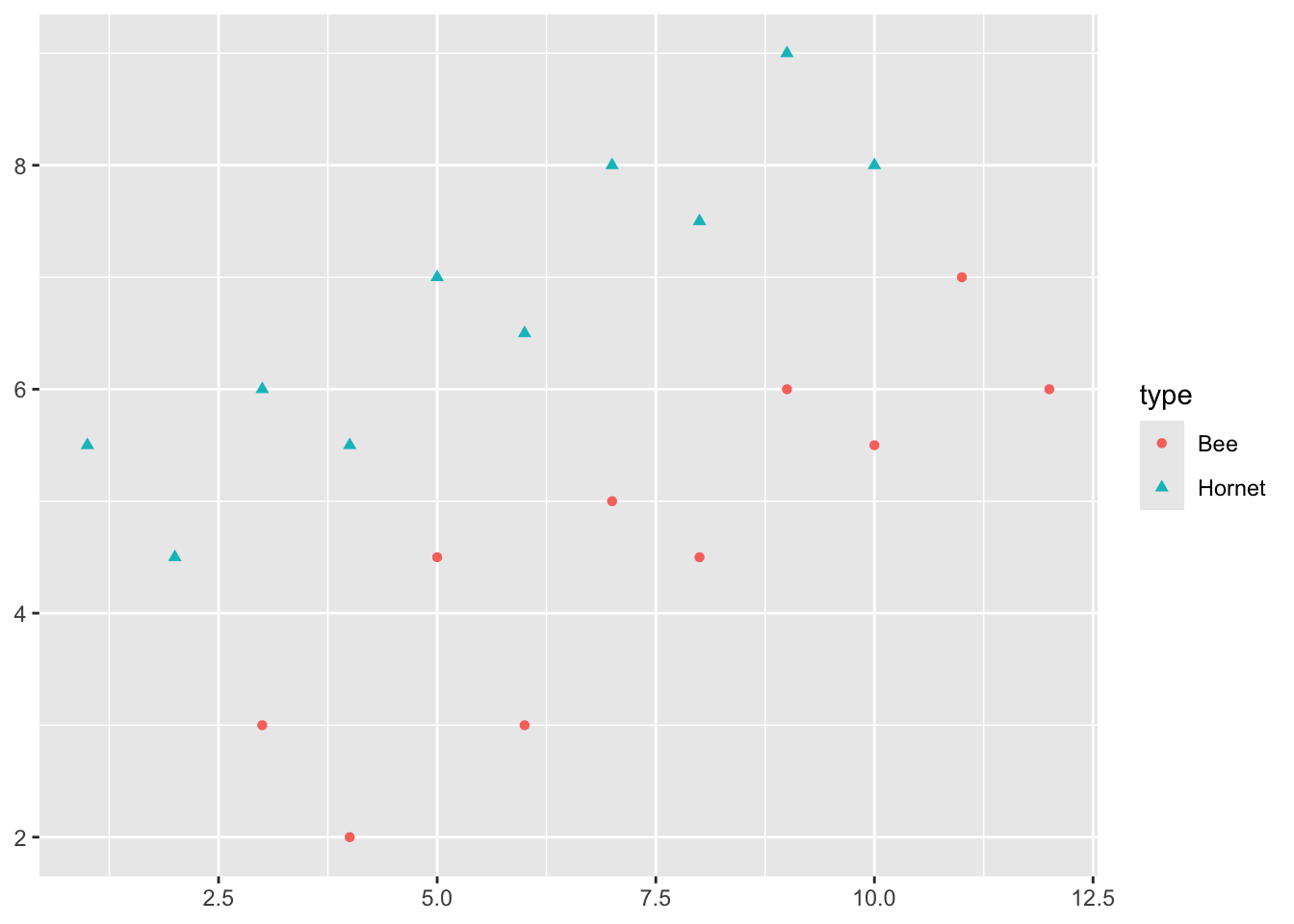
Say we have two responses, e.g., \(Y = 1\) means a Hornet and \(Y = -1\) means a Bee.
We want to be able to clearly classify a new insect as a Hornet or a Bee.
It looks like I can draw a line in the gap between the points to separate the Hornets and Bees.
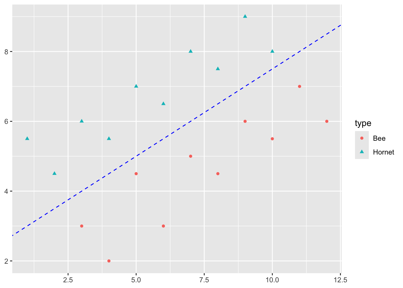
In fact I can draw multiple lines in the gap between the points to separate the Hornets and Bees.
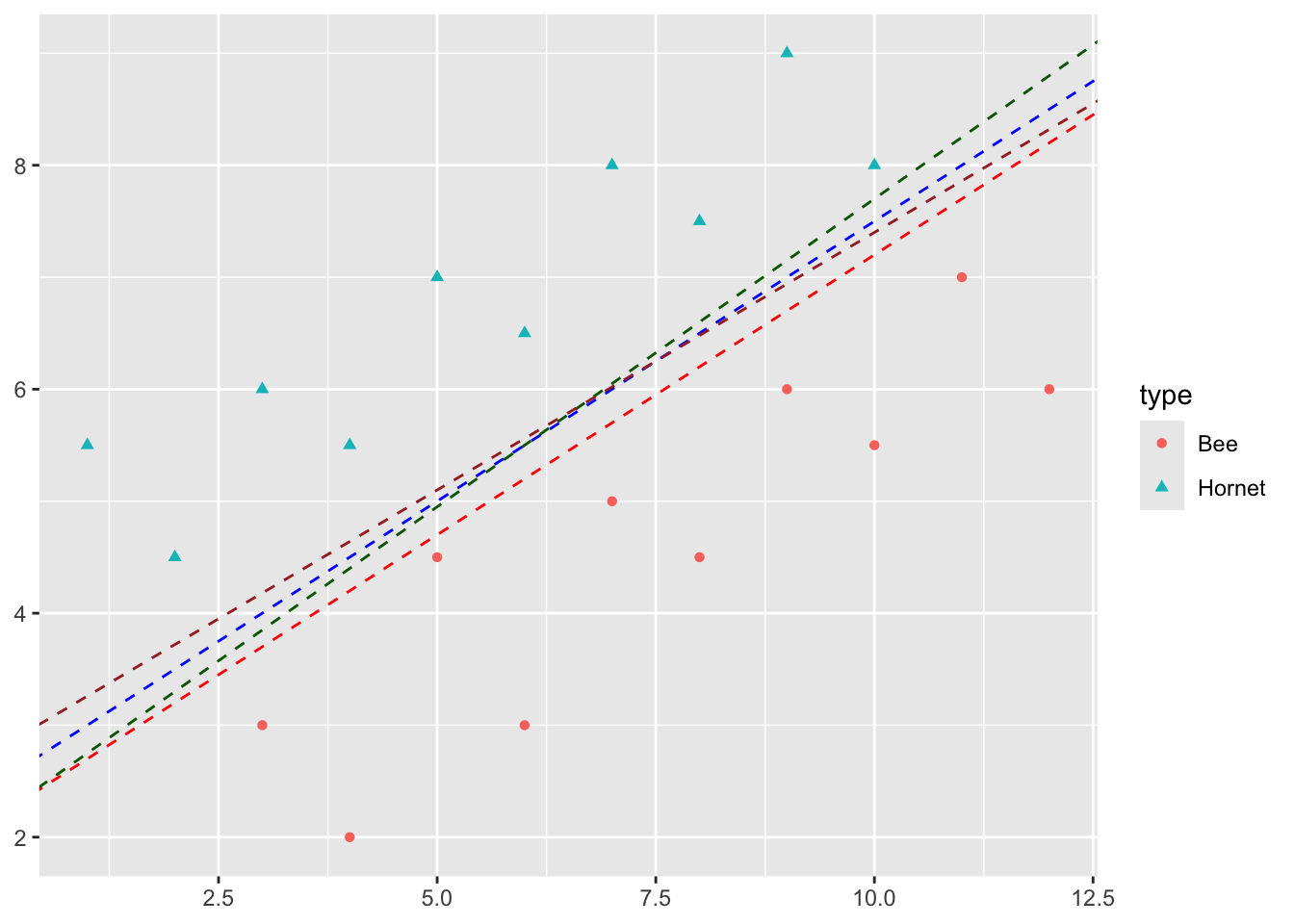
Some of these lines have points close to them which suggests I am less sure about the prediction there.
- Maybe it is a young hornet so it looks like a young bee?
- If the point is far from the line, I am pretty confident it is a hornet or it is a bee.
So intuitively, I would like all points to be as far as possible from the line.
The best classifier maximizes the margin \(M\) where the margin is the distance from the line to the point closest to the line.
9.2.1 Inner Products
Inner products are used in computing the maximum marginal classifier as they provide both an algebraic and computational path to a solution.
We can think of the inner product of two vectors (a generalization of the dot product) as a scalar representing the angle \(\phi\) (phi) between two vectors.
\[<\vec{a}, \vec{b}> =||\vec{a}||\, ||\vec{b}|| \text{cos}\phi.\]
where \(||\vec{a}||\) is the length of the vector.
The inner product in our case can also be defined as
\[<\vec{a}, \vec{b}> = \sum_{i=1}^p a_ib_i = a_1b_1 + a_2b_2 + \cdots + a_pb_p. \tag{9.1}\]
- If \(\vec{a}\) and \(\vec{b}\) are orthogonal, then \(\cos(\phi) = 0\) so \(<\vec{a}, \vec{b}> = 0.\)
- It is also true that the projection of \(\vec{a}\) onto another vector \(\vec{b}\), call it \(\vec{a}_\vec{b}\), is \(||\vec{a}|| \text{cos}\, \phi\).
9.2.2 Deriving the Maximum Marginal Classifier (MMC)
Let’s call the MMC line separating our two sets of points (bees and hornets) \(H\), for the separating hyperplane needed with more than three dimensions (1 + \(p\)).
Given a \(p\)-dimensional space, a hyperplane is a flat affine subspace of dimension \(p-1\).
- For \(p=2\) dimensions, the hyperplane is a line as seen in Figure 9.1.
- For \(p=3\) dimensions, the hyperplane has dimension 2 so is a flat plane.
- For \(p>3\) dimensions, we call it a hyperplane of dimension \(p-1\) and it is still “flat”.
We can define a hyperplane as a linear combination of \(X_i\). In two dimensions that gives us:
\[ \beta_0 + \beta_1X_1 + \beta_2X_2 = 0 \tag{9.2}\]
Equation 9.2 can be see as the formula for a line as any point \((X_1, X_2)\) that satisfies the equation is on the line.
- Figure 9.1 shows multiple lines (hyperplanes) where each has its own set of \(\beta\)s.
In \(p\) dimensions, we simply extend Equation 9.2 to define the hyperplane \(H\) as
\[ \beta_0 + \beta_1X_1 + \beta_2X_2 + \cdots + \beta_pX_p= 0 \tag{9.3}\]
Given we have a hyperplane \(H\) as defined in Equation 9.3 with a fixed set of \(\beta\)s then:
- if \(\beta_0 + \beta_1X_1 + \beta_2X_2 + \cdots + \beta_pX_p> 0\) for a point \(\vec{X}\) the point \(\vec{X}\) is “above” the hyperplane, and,
- if \(\beta_0 + \beta_1X_1 + \beta_2X_2 + \cdots + \beta_pX_p< 0\) for a point \(\vec{X}\) the point \(\vec{X}\) is “below” the hyperplane.
- If \(\beta_0 + \beta_1X_1 + \beta_2X_2 + \cdots + \beta_pX_p >> 0\) the point is “far” above the plane and the same if it is much less than 0, it is far away from \(H\) on the other side.
We can use Equation 9.3 to find the distance from any point \(\vec{X}\) in our data to \(H\).
The margin, \(M\), is the shortest distance from any point \(\vec{X}\) to \(H\).
- That distance will be from the \(\vec{X}\) to the point \(\vec{X}_H\) in the hyperplane that is the projection of \(\vec{X}\) onto the plane \(H\).
We want to maximize \(M\) while ensuring that all points are on the correct side of the hyperplane.
More formally, lets define our response as \(Y = \pm 1\).
- Then we can see that
\[ \begin{array} \\ \beta_0 + \beta_1X_1 + \beta_2X_2 + \cdots + \beta_pX_p> 0 \iff Y = 1 \\ \beta_0 + \beta_1X_1 + \beta_2X_2 + \cdots + \beta_pX_p< 0 \iff Y= -1 \end{array} \tag{9.4}\]
We can combine the two equations in Equation 9.4 to get
\[ Y(\beta_0 + \beta_1X_1 + \beta_2X_2 + \cdots + \beta_pX_p)> 0. \tag{9.5}\]
If the \(\beta\)s are for a separating hyperplane, then Equation 9.5 is true for all values of \(\vec{Y}\) and \(\vec{X}\) in our data set.
We normalize the \(\beta\) in Equation 9.5 by requiring \(||\beta||^2 = \sum\beta_j^2 = 1\) so we have a unique definition of the separating hyperplane.
That allows us to express the distance between the hyperplane \(H\) and a point \(\vec{X}\) as an inner product using Equation 9.1 to get
\[\text{dist}(\vec{X}, H) = \beta_1 X_1 + \cdots + \beta_p X_p. \tag{9.6}\]
Given the vector \(\vec{\beta}\), we can construct the hyperplane \(H\) so it is orthogonal to the vector \(\vec{\beta}\).
- This means the inner product of \(\vec{\beta}\) with any point \(\vec{X}_H\) that lies in the hyperplane is 0.
\[\forall\vec{X} \in H \quad <\vec{\beta}, \vec{X}> = \beta_1 X_1 + \cdots + \beta_p X_p = 0.\] Points not on the hyperplane then have inner product values that are non-zero as seen in Equation 9.4.
- For points on one side of the plane, the distance is positive (where \(Y = 1\)).
- For points on the other side, the distance is defined as negative (where \(Y = -1\)).
For all points \(\vec{X}\), the inner product between \(\vec{X}\) and \(\vec{\beta}\) is then
\[<\vec{\beta}, \vec{X}> = \underbrace{||\vec{\beta}||}_{= 1}\cdot\underbrace{||\vec{X}||\cos(\phi)}_\text{adjacent side} = \text{dist}(\vec{X}, H) \tag{9.7}\]
where \(\phi\) (phi) is the angle between \(\vec{\beta}\) and \(\vec{X}\).
We want to maximize \(M\) subject to \(\sum\beta_j^2 = 1\).
So to maximize the margin \(M\) means maximizing the inner product in Equation 9.7, which is equivalent to the need to find the \(\beta\)s which maximize Equation 9.6.
The Maximal Margin Classifier is the hyperplane \(H\) that maximizes the margin \(M\) such that the minimum distance between \(\vec{X}\) and \(H\) \(\times\) the response value is positive and that minimum distance is \(\geq M\).
\[ \underbrace{\text{min}}_{\vec{\beta}}\underbrace{(\beta_0 + \beta_1 X_1 + \cdots + \beta_p X_p)}_{ >0 \text{ on one side} \\ < 0 \text{ on the other side}}\underbrace{Y_i}_{\pm 1} \geq M \tag{9.8}\] and \(\sum_1^p\beta_j^2 = 1\).
We need to find the values of \(\vec{\beta}\) out of all possible hyperplanes that provide the maximum value for \(M\).
This can be expressed as an equivalent quadratic optimization problem with linear constraints for which there are many solvers which can find the solution.
Looking at our picture, we can manually find the \(\beta\)s by adjusting the intercept and slope to get a maximum margin \(M\).
- Adjust the intercept of the separating line until it just touches the closet point for one class of response.
- Adjust the slope so it touches two points for that class.
- Create a second line with the same slope and adjust the intercept so it touches the closest point in the other class of responses.
- This is the maximum distance between the lines, so the maximal margin classifier is the line with the intercept exactly in the middle of the intercepts of two lines and with the same slope.
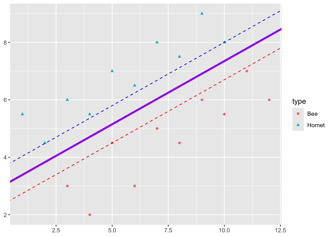
The three points \(\vec{X_1}, \vec{X_2}, \vec{X}_3\) that we just identified are the Support Vectors for this classifier.

However, the Maximal Marginal Classifier usually does not exist as the data cannot be cleanly separated.
That is why SVM machines have gotten more sophisticated to allow for less restrictive boundaries and allow for points that are misclassified.
The following is an example where the the points overlap so the algorithm has to use a more general method.
9.2.3 Example SVM in R
We will use the package {e1071} to build an SVM using the HOME_SALES.CSV data.
homes <- read_csv("https://raw.githubusercontent.com/rressler/data_raw_courses/main/HOME_SALES.csv", show_col_types = FALSE)
# Assign the levels to homes so Quality is in the right order.
homes$QUALITY <- factor(homes$QUALITY, levels = c("LOW", "MEDIUM", "HIGH"))
names(homes)
[1] "ID" "SALES_PRICE" "FINISHED_AREA" "BEDROOMS"
[5] "BATHROOMS" "GARAGE_SIZE" "YEAR_BUILT" "STYLE"
[9] "LOT_SIZE" "AIR_CONDITIONER" "POOL" "QUALITY"
[13] "HIGHWAY" [1] "LOW" "MEDIUM" "HIGH" Let’s look at QUALITY as a function of SALES_PRICE and YEAR_BUILT.
Show code
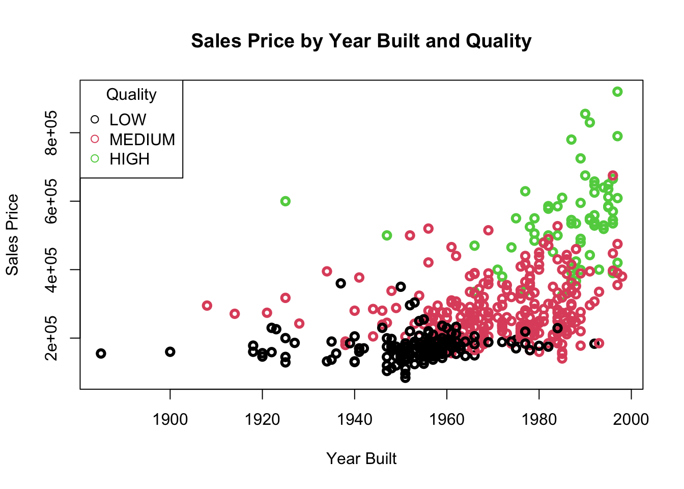
We want to separate with hyperplanes. We see that we cannot do it with a MMC as there is none, the points overlap.
Let’s load the package and predict QUALITY as a function of SALES_PRICE and YEAR_BUILT built using the defaults in e1071::svm().
Call:
svm(formula = as.factor(QUALITY) ~ SALES_PRICE + YEAR_BUILT, data = homes)


Parameters:
   SVM-Type:  C-classification
 SVM-Kernel:  radial
       cost:  1

Number of Support Vectors:  255
It chose the kernel, the type of boundary, to be radial.
Let’s set kernel = "linear".
Call:
svm(formula = as.factor(QUALITY) ~ SALES_PRICE + YEAR_BUILT, data = homes,
    kernel = "linear")


Parameters:
   SVM-Type:  C-classification
 SVM-Kernel:  linear
       cost:  1

Number of Support Vectors:  248
If we try to plot directly it will error out as there are more variables in the data frame identified in the function, than the two predictors used in the model.
- We can just adjust the data sent to
plot(). -
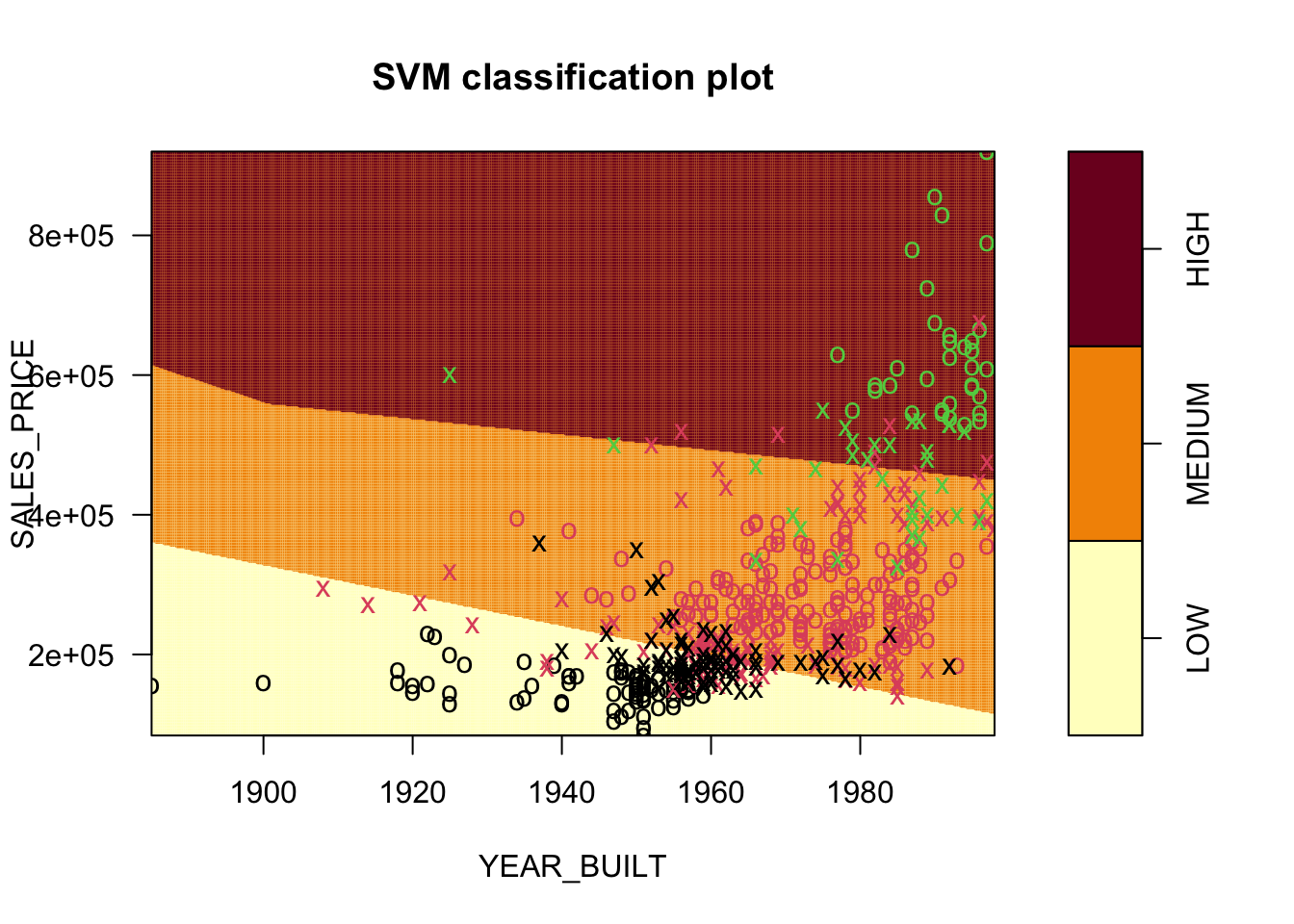
plot.svm()produces a contour plot by default showing the regions.
- The points are color coded according to the actual response.
- The
xshapes are the points that are the support vectors. - These are the 248 Support Vectors identified in
SVM.SV.
If we use a different kernel, we will get different results.
Here the default choice of a radial kernel.
Call:
svm(formula = as.factor(QUALITY) ~ SALES_PRICE + YEAR_BUILT, data = homes,
    kernel = "radial")


Parameters:
   SVM-Type:  C-classification
 SVM-Kernel:  radial
       cost:  1

Number of Support Vectors:  255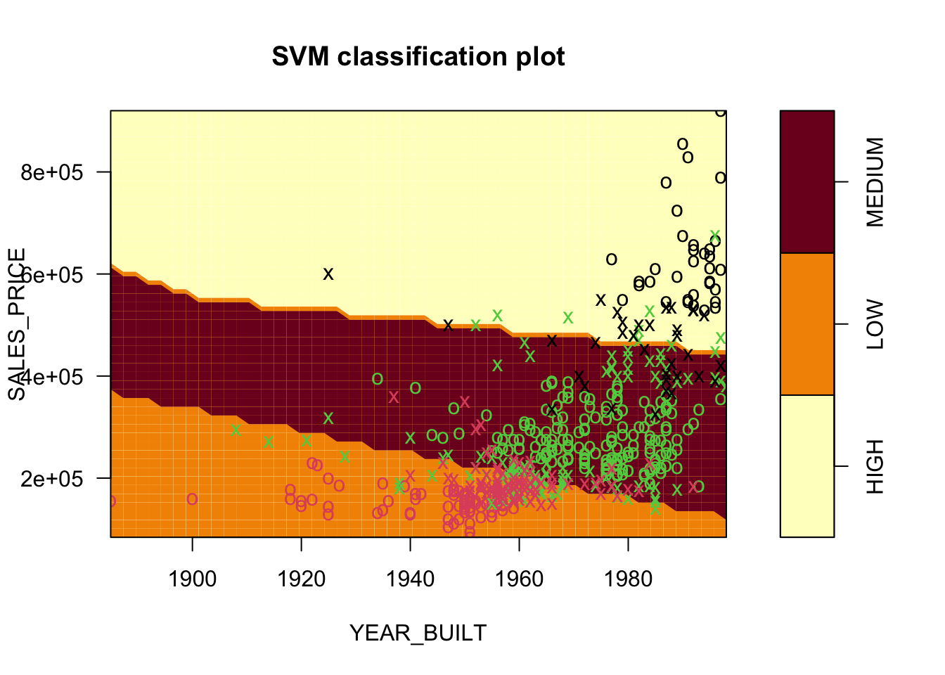
9.3 Support Vector Classifier
We have seen the the MMC has several disadvantages:
- It can “bee” too sensitive or too flexible. The MMC uses a minimal number of points (SVs) to determine the classifier and these can be highly influential points. What if one of them is wrong?
- As an example, you have 50,000 bees and hornets and only two hornets and one bee determine the classifier.
- Adding a new bee or losing a hornet point can create large changes in the parameter estimates.
- The MMC hyperplane, with no violators, may not exist (when the data overlaps).
To respond to these we need to do two things:
Allow for imperfect separation to make it more flexible.
Increase the number of Support Vectors to reduce the potential for few high-influence SVs.
To make the SVM more flexible, (and enable it to exist) we want to allow for observations that violate the boundary (at a cost) within a given total cost \(C\), a tuning parameter.
- This means we want to relax Equation 9.8 as it required all points to be on one side or the other of the boundary.
A Support Vector Classifier maximizes the margin \(M\) subject to:
\[ Y_i (\beta_0 + \beta_1 X_{1i} + \cdots + \beta_p X_{pi})\geq M (1 - \epsilon_i) \tag{9.9}\]
where \(\epsilon\) is some small number and \(\sum_1^p\beta_j^2 = 1\).
The \(\epsilon_i\) are called slack variables and they are what allow for the violations of the boundary.
- These have to be bounded so we have to add a third and fourth constraint
\[\epsilon_i \geq 0 \,\,\forall i \quad \text{and }\sum_{i = 1}^{n}\epsilon_i \leq C \quad \leftarrow \text{the Cost budget}. \tag{9.10}\]
- If \(\epsilon_i = 0\), then the point is classified correctly and clears the margin.
- If \(\epsilon_i > 1\), then Equation 9.9 is negative and the data point is misclassified.
- The total number of misclassified points cannot exceed \(C\).
- If \(C\) = 0 then no points can be misclassified and we are back to an MMC (if it exists).
The use of \(C\) in Equation 9.10 is to align with the svm parameter cost. This is from the “regularization” term in the Lagrangian formulation of the dual problem for the optimization. Larger \(C\) means more freedom to misclassify points.
You will see many other presentations where the \(C\) term is the penalty parameter in the optimization (like \(\lambda\) in ridge/lasso so large \(C\) is means higher cost of misclassification.
It can be confusing to reconcile the two exact opposite presentations so read carefully.
The use of the slack variables for a support vector classifier is also known as a “soft-boundary” classifier.
The optimization uses a hinge-loss function to penalize points that are less than \(M\) from the hyperplane or even on the incorrect side of the hyperplane.
- The hinge loss function is one of several kinds of loss functions used in machine learning.
- The use of a hinge loss function differentiates SVM from Logistic Regression which uses the the logistic loss function.
The shift to using a hinge-loss converts the optimization from maximizing the margin \(M\) to minimizing the loss associated with the trade off between a smaller margin (fewer training data points misclassified) and a larger margin (fewer testing points misclassified).
The smaller the margin, the greater of a “squiggly” hyperplane in \(p\) dimensions which leads to overfitting, decreasing bias but increasing variance.
The larger the margin, the less “squiggly” the hyperplane which will reduce performance on training but may be better on testing, increasing bias but decreasing variance.
The common bias-variance trade off is present here and can be addressed through tuning.
This is an SVC. If you allow nonlinear boundaries, then it becomes a Support Vector Machine.
9.4 Support Vector Machines
SVMs are Support Vector Classifiers which allow non-linear boundaries.
People use the word kernel to describe the possibility to generalize \(\sum\beta_j X_j = <\vec{\beta}, \vec{X}>\).
- When a linear kernel is used, the optimization is about inner products and the hyperplane \(H\) is determined by inner products of linear kernels of \(X\) (the boundary) and \(X_i\) the data.
The \(\sum\beta_j X_j\) is a linear kernel.
As we have seen, there are multiple kernels that can be nonlinear transformations.
- Radial Kernel: \(e^{-\gamma\sum(x - x_i)^2}\). The radial kernel is the most widely used kernel for classifying datasets that cannot be separated linearly.
- Polynomial Kernel: \((1 + \sum_j X_jX_{ij})^d\) for some power \(d\).
- Sigmoid Kernel: The S-shaped function.\(K(x,x_i) = tanh(\alpha x_i\cdot x_j +\beta)\). This is more common in neural networks than SVM.
The use of kernels, the kernel trick, is an approach used in multiple machine learning methods to map a set of points in \(p\) dimensions to a higher-order dimension where the structure may be easier to see.
- Consider the use of polynomial terms in linear regression where you are increasing the dimension by each additional polynomial term without adding new data.
- The kernel trick is to map the data into the higher dimension, find the hyperplane there, and then map back to the original \(p\) dimensions where the hyperplane gets transformed into the curves or ellipses.
Choice of kernel is also a tuning parameter.
9.5 Example in R
Let’s load the libraries for SVM {e1071} and for the college data from {ISLR2}.
 [1] "Private"     "Apps"        "Accept"      "Enroll"      "Top10perc"
 [6] "Top25perc"   "F.Undergrad" "P.Undergrad" "Outstate"    "Room.Board"
[11] "Books"       "Personal"    "PhD"         "Terminal"    "S.F.Ratio"
[16] "perc.alumni" "Expend" "Grad.Rate" Private Apps Accept Enroll Top10perc
No :212 Min. : 81 Min. : 72 Min. : 35 Min. : 1.00
Yes:565 1st Qu.: 776 1st Qu.: 604 1st Qu.: 242 1st Qu.:15.00
Median : 1558 Median : 1110 Median : 434 Median :23.00
Mean : 3002 Mean : 2019 Mean : 780 Mean :27.56
3rd Qu.: 3624 3rd Qu.: 2424 3rd Qu.: 902 3rd Qu.:35.00
Max. :48094 Max. :26330 Max. :6392 Max. :96.00
Top25perc F.Undergrad P.Undergrad Outstate
Min. : 9.0 Min. : 139 Min. : 1.0 Min. : 2340
1st Qu.: 41.0 1st Qu.: 992 1st Qu.: 95.0 1st Qu.: 7320
Median : 54.0 Median : 1707 Median : 353.0 Median : 9990
Mean : 55.8 Mean : 3700 Mean : 855.3 Mean :10441
3rd Qu.: 69.0 3rd Qu.: 4005 3rd Qu.: 967.0 3rd Qu.:12925
Max. :100.0 Max. :31643 Max. :21836.0 Max. :21700
Room.Board Books Personal PhD
Min. :1780 Min. : 96.0 Min. : 250 Min. : 8.00
1st Qu.:3597 1st Qu.: 470.0 1st Qu.: 850 1st Qu.: 62.00
Median :4200 Median : 500.0 Median :1200 Median : 75.00
Mean :4358 Mean : 549.4 Mean :1341 Mean : 72.66
3rd Qu.:5050 3rd Qu.: 600.0 3rd Qu.:1700 3rd Qu.: 85.00
Max. :8124 Max. :2340.0 Max. :6800 Max. :103.00
Terminal S.F.Ratio perc.alumni Expend
Min. : 24.0 Min. : 2.50 Min. : 0.00 Min. : 3186
1st Qu.: 71.0 1st Qu.:11.50 1st Qu.:13.00 1st Qu.: 6751
Median : 82.0 Median :13.60 Median :21.00 Median : 8377
Mean : 79.7 Mean :14.09 Mean :22.74 Mean : 9660
3rd Qu.: 92.0 3rd Qu.:16.50 3rd Qu.:31.00 3rd Qu.:10830
Max. :100.0 Max. :39.80 Max. :64.00 Max. :56233
Grad.Rate
Min. : 10.00
1st Qu.: 53.00
Median : 65.00
Mean : 65.46
3rd Qu.: 78.00
Max. :118.00 Let’s use Private as our response with predictors Expend and S.F.Ratio.
- Create a collapsed data set for plotting.
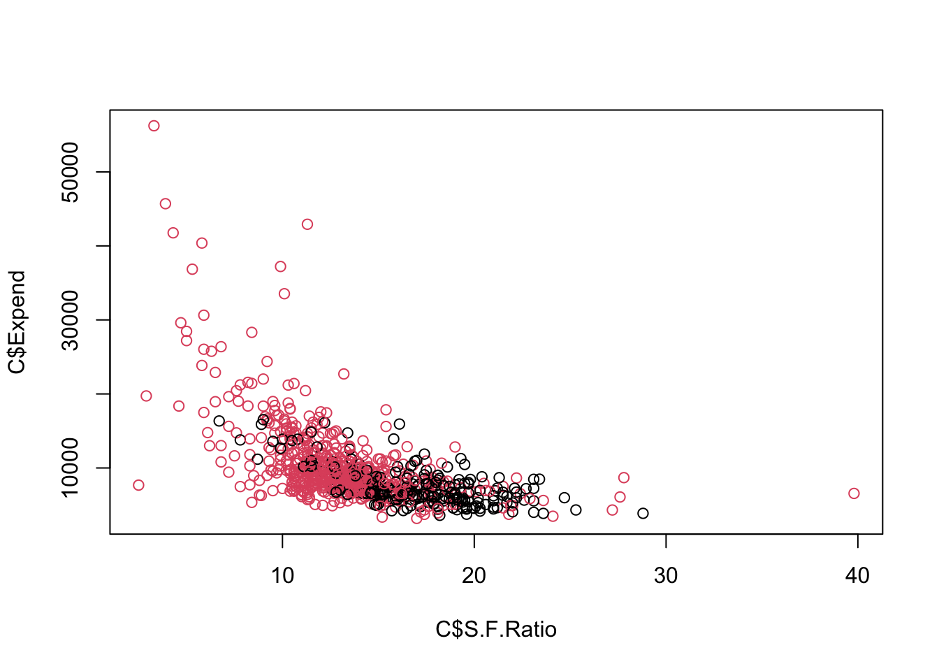
Let’s plot.
The Maximal Margin Classifier does not appear to exist - Why?
Let’s use a linear kernel SVC.
- We can plot since it is only two predictors.
SVM <- svm(Private ~ Expend + S.F.Ratio, data = C, kernel = "linear")
plot(SVM, data = C, color.palette = topo.colors, grid = 400)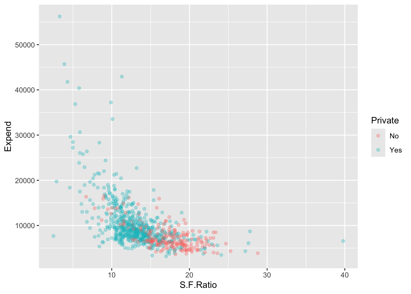
All the points marked by an x are support vectors.
- We can see there are 381 of them.
Call:
svm(formula = Private ~ Expend + S.F.Ratio, data = C, kernel = "linear")


Parameters:
   SVM-Type:  C-classification
 SVM-Kernel:  linear
       cost:  1

Number of Support Vectors:  381
Let’s predict and tabulate the classification error rate.
Yhat   No Yes
  No   99  47
Yes 113 518[1] 0.7940798Can we do better?
Let’s try with more data and a linear kernel.
We can’t plot all the boundaries, but we can look at two variables at a time using formula notation.
You can also reset the default values for one or more of the other variables using the slice = argument.
Show code
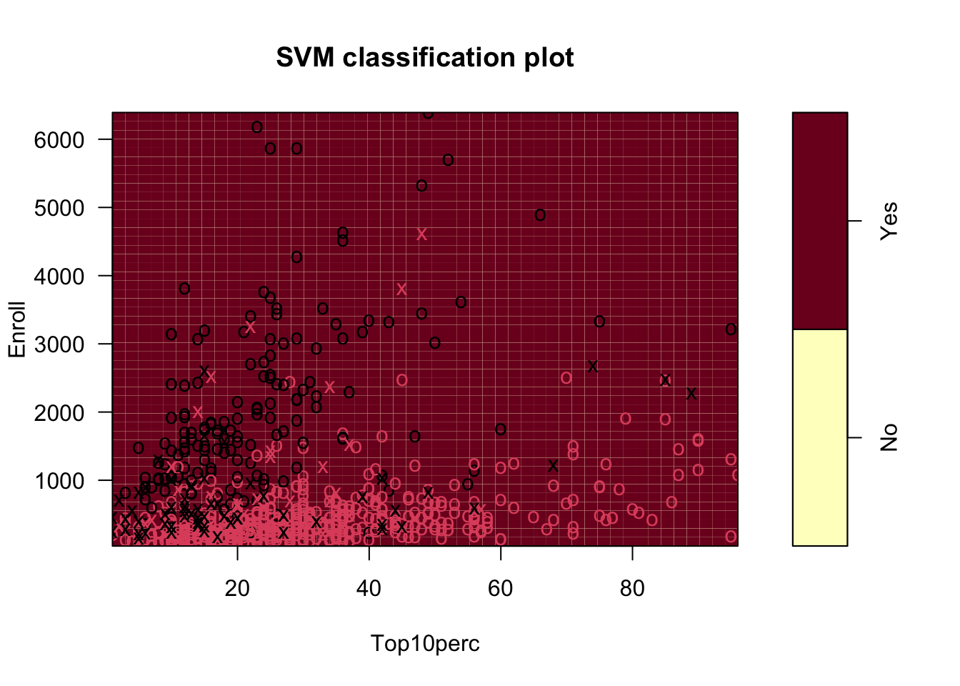
We can predict and get a classification rate on the training data.
Yhat_all  No Yes
     No  188  18
Yes 24 547[1] 0.9459459Good improvement. Can we do better?
9.5.1 Tuning an SVM Based on the Kernel
There is a built-in function tune() for tuning across different kernels with a default for comparison based on cross-validation for which the tune.control() function provides options.
- The default is \(K=10\)-fold cross validation.
You can control the parameters used for the tuning using tune.control().
- The default for
samplingis cross-validation. - The default for
sampling.aggregateis mean (for the error). - The default for
sampling.dispersionis standard deviation.
Parameter tuning of 'svm':

- sampling method: 10-fold cross validation

- best parameters:
 kernel
 linear

- best performance: 0.05794206 [1] 0.9420579Note the best kernel was still linear but the error rate dropped slightly - Why?
- This is a prediction error rate based on the default of \(K=10\)-fold cross-validation.
We can look at how kernel each performed in terms of the prediction error rate using summary.svm().
Parameter tuning of 'svm':

- sampling method: 10-fold cross validation

- best parameters:
 kernel
 linear

- best performance: 0.05794206

- Detailed performance results:
      kernel      error dispersion
1     linear 0.05794206 0.01260768
2 polynomial 0.09015984 0.03225296
3     radial 0.06829837 0.02602873
4    sigmoid 0.09140859 0.02745598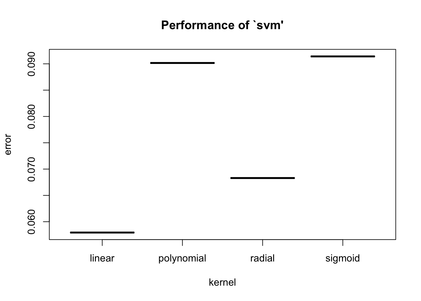
[1] 0.94205799.5.2 Tuning an SVM Based on Kernel and Cost Budget
We can also tune based on the Kernel and the Cost Budget \(C\).
Let’s consider cost budgets ranging from .1 to 3.0 along with the various kernels.
- This creates 120 different combinations that are explored using grid search.
Let’s see the results.
Parameter tuning of 'svm':

- sampling method: 10-fold cross validation

- best parameters:
 cost kernel
  0.8 linear

- best performance: 0.05537796

- Detailed performance results:
    cost     kernel      error dispersion
1    0.1     linear 0.06438561 0.02192569
2    0.2     linear 0.06055611 0.01945292
3    0.3     linear 0.05799201 0.01968321
4    0.4     linear 0.05797536 0.01960414
5    0.5     linear 0.05794206 0.01638690
6    0.6     linear 0.05666001 0.01394147
7    0.7     linear 0.05794206 0.01260768
8    0.8     linear 0.05537796 0.01376943
9    0.9     linear 0.05666001 0.01394147
10   1.0     linear 0.05794206 0.01260768
11   1.1     linear 0.05537796 0.01237221
12   1.2     linear 0.05795871 0.01273033
13   1.3     linear 0.05795871 0.01273033
14   1.4     linear 0.05666001 0.01101422
15   1.5     linear 0.05666001 0.01101422
16   1.6     linear 0.05666001 0.01101422
17   1.7     linear 0.05666001 0.01101422
18   1.8     linear 0.05666001 0.01101422
19   1.9     linear 0.05666001 0.01101422
20   2.0     linear 0.05666001 0.01101422
21   2.1     linear 0.05537796 0.01079564
22   2.2     linear 0.05666001 0.01101422
23   2.3     linear 0.05667666 0.01268834
24   2.4     linear 0.05795871 0.01273033
25   2.5     linear 0.05795871 0.01273033
26   2.6     linear 0.05667666 0.01268834
27   2.7     linear 0.05795871 0.01273033
28   2.8     linear 0.05795871 0.01273033
29   2.9     linear 0.05924076 0.01400006
30   3.0     linear 0.05924076 0.01400006
31   0.1 polynomial 0.16858142 0.04497459
32   0.2 polynomial 0.14415584 0.04101103
33   0.3 polynomial 0.12099567 0.03694937
34   0.4 polynomial 0.11585082 0.03786331
35   0.5 polynomial 0.10945721 0.03915616
36   0.6 polynomial 0.09915085 0.03702401
37   0.7 polynomial 0.09144189 0.03724379
38   0.8 polynomial 0.09402264 0.03655571
39   0.9 polynomial 0.09402264 0.03655571
40   1.0 polynomial 0.09015984 0.03225296
41   1.1 polynomial 0.08887779 0.03308174
42   1.2 polynomial 0.08629704 0.03447791
43   1.3 polynomial 0.08757909 0.03379247
44   1.4 polynomial 0.08628039 0.03277538
45   1.5 polynomial 0.08371628 0.03062042
46   1.6 polynomial 0.08241758 0.02993723
47   1.7 polynomial 0.08373293 0.02948860
48   1.8 polynomial 0.08501499 0.03182319
49   1.9 polynomial 0.08373293 0.03129145
50   2.0 polynomial 0.08245088 0.02885072
51   2.1 polynomial 0.08115218 0.02871968
52   2.2 polynomial 0.07858808 0.03024341
53   2.3 polynomial 0.07858808 0.03024341
54   2.4 polynomial 0.07730603 0.03059156
55   2.5 polynomial 0.07730603 0.02810233
56   2.6 polynomial 0.07602398 0.02904814
57   2.7 polynomial 0.07472527 0.02924351
58   2.8 polynomial 0.07472527 0.02924351
59   2.9 polynomial 0.07472527 0.02924351
60   3.0 polynomial 0.07472527 0.02924351
61   0.1     radial 0.08116883 0.04627136
62   0.2     radial 0.07217782 0.03814516
63   0.3     radial 0.07474192 0.03543490
64   0.4     radial 0.07345987 0.03453698
65   0.5     radial 0.06958042 0.03236100
66   0.6     radial 0.06958042 0.03236100
67   0.7     radial 0.06573427 0.02898621
68   0.8     radial 0.06573427 0.02898621
69   0.9     radial 0.06573427 0.02898621
70   1.0     radial 0.06829837 0.02602873
71   1.1     radial 0.06958042 0.02467643
72   1.2     radial 0.06443556 0.02734751
73   1.3     radial 0.06573427 0.02564316
74   1.4     radial 0.06573427 0.02564316
75   1.5     radial 0.06573427 0.02564316
76   1.6     radial 0.06443556 0.02528367
77   1.7     radial 0.06443556 0.02528367
78   1.8     radial 0.06187146 0.02792775
79   1.9     radial 0.06187146 0.02792775
80   2.0     radial 0.06317016 0.02838427
81   2.1     radial 0.06058941 0.02606736
82   2.2     radial 0.06058941 0.02606736
83   2.3     radial 0.06187146 0.02587329
84   2.4     radial 0.06058941 0.02809064
85   2.5     radial 0.06058941 0.02809064
86   2.6     radial 0.06058941 0.02809064
87   2.7     radial 0.06188811 0.02925701
88   2.8     radial 0.06188811 0.02925701
89   2.9     radial 0.06058941 0.02809064
90   3.0     radial 0.06058941 0.02809064
91   0.1    sigmoid 0.07470862 0.03031604
92   0.2    sigmoid 0.07084582 0.02871185
93   0.3    sigmoid 0.07214452 0.02605821
94   0.4    sigmoid 0.07983683 0.03256111
95   0.5    sigmoid 0.08626374 0.02581790
96   0.6    sigmoid 0.08624709 0.02971032
97   0.7    sigmoid 0.08626374 0.02976102
98   0.8    sigmoid 0.08752914 0.03015130
99   0.9    sigmoid 0.09137529 0.02525171
100  1.0    sigmoid 0.09140859 0.02745598
101  1.1    sigmoid 0.09140859 0.02609176
102  1.2    sigmoid 0.09398934 0.02440441
103  1.3    sigmoid 0.09142524 0.02618232
104  1.4    sigmoid 0.09398934 0.02364423
105  1.5    sigmoid 0.09140859 0.02393977
106  1.6    sigmoid 0.08884449 0.02882662
107  1.7    sigmoid 0.08884449 0.02882662
108  1.8    sigmoid 0.09012654 0.02653054
109  1.9    sigmoid 0.09527140 0.02453213
110  2.0    sigmoid 0.09655345 0.02301004
111  2.1    sigmoid 0.10039960 0.02257454
112  2.2    sigmoid 0.09911755 0.02358825
113  2.3    sigmoid 0.09911755 0.02358825
114  2.4    sigmoid 0.09527140 0.02800810
115  2.5    sigmoid 0.09783550 0.02593453
116  2.6    sigmoid 0.09781885 0.02654484
117  2.7    sigmoid 0.09781885 0.02654484
118  2.8    sigmoid 0.09525475 0.02857250
119  2.9    sigmoid 0.09525475 0.02792601
120 3.0 sigmoid 0.09525475 0.02658591[1] 0.944622 0.944622Let’s create the final “Best” model.
Call:
svm(formula = Private ~ ., data = College, kernel = "linear", cost = 0.8)


Parameters:
   SVM-Type:  C-classification
 SVM-Kernel:  linear
       cost:  0.8

Number of Support Vectors:  127

 ( 65 62 )


Number of Classes:  2

Levels:
 No Yes
127 Support vectors, 65 on the No side and 62 on the Yes side.
The tune function makes it straightforward to tune the SVM.
SVMs are a useful method for classification and can also be used for regression.
See Applications of SVM in the Real World.
Careful tuning can help with selection of the right kernel and cost budget for the data.
